White dwarfs stripped by massive black holes: sources of coincident gravitational and electromagnetic radiation

Abstract

White dwarfs inspiraling into black holes of mass $M_{\rm BH}\lower 2.15277pt\hbox{$\;\buildrel>\over{\sim}\;$}10^{5}M_{\odot}$ are detectable sources of gravitational waves in the LISA band. In many of these events, the white dwarf begins to lose mass during the main observational phase of the inspiral. The mass loss starts gently and can last for thousands of orbits. The white dwarf matter overflows the Roche lobe through the $L_{1}$ point at each pericenter passage and the mass loss repeats periodically. The process occurs very close to the black hole and the released gas can accrete, creating a bright source of radiation with luminosity close to the Eddington limit, $L\sim 10^{43}$ erg s^-1. This class of inspirals offers a promising scenario for dual detections of gravitational waves and electromagnetic radiation.

1 Introduction

One of the goals of the Laser Interferometer Space Antenna (LISA) mission is to detect gravitational waves from compact stellar objects spiraling into massive black holes, a class of events called extreme-mass-ratio inspirals (EMRIs) (e.g., Hils & Bender 1995; Gair et al. 2004; Barack & Cutler 2004; see Hughes 2009 and Sathyaprakash & Schutz 2009 for recent reviews). Of particular interest are sources of coincident gravitational and electromagnetic radiation. Besides providing unique information on the nature of the event, such dual detections will lead to a new version of Hubble diagram that is based on the gravitational distance measurements (e.g. Bloom et al. 2009; Phinney 2009).

Inspirals into black holes of masses $M_{\rm BH}\sim(10^{5}-10^{6})M_{\odot}$ produce gravitational waves in the frequency band where LISA is most sensitive. Normal stars are tidally disrupted well before they approach such black holes, and therefore discounted as possible LISA sources (however, see Freitag 2003). Inspirals of compact objects are guaranteed sources of gravitational waves, however most of them are not promising for dual detections. In particular, stellar-mass black hole or neutron star inspirals are not expected to generate bright electromagnetic signals. Only inspiraling white dwarfs (WDs) offer a possibility for dual detection (Menou et. al. 2008; Sesana et al. 2008). WDs can be tidally disrupted very close to the black hole and then could create a transient accretion disc with Eddington luminosity.

Estimated EMRI rates are high enough for observations with LISA (e.g. Phinney 2009). The expected fraction of WD inpirals among all EMRIs depends on the degree of mass segregation in galactic nuclei, which favors stellar-mass black holes over white dwarfs in the central cluster. The abundance of white dwarfs also depends on the details of stellar evolution, which are not completely understood. A fraction of WD inpirals as large as $\sim 10\%$ has been suggested (e.g. Hopman & Alexander 2006a).

The orbital parameters of WD inspirals are also uncertain. EMRIs form when a compact object is captured onto a tight orbit whose evolution is controlled by gravitational radiation rather than random interactions with other stars in the central cluster around the massive black hole. Two main channels exist for EMRI formation: capture of single stars and capture of binary systems (e.g., Hils & Bender 1995; Sigurdsson & Rees 1997; Ivanov 2002; Gair et al. 2004; Hopman & Alexander 2005, 2006a,b, 2007; Miller et al. 2005; Hopman 2009). In the single-capture scenario, the shrinking orbit can retain a significant eccentricity until the end of inspiral. In contrast, the binary-capture scenario leads to nearly circular orbits (Miller et al. 2005).

In this paper, we focus on WD inspirals that are not completed because the star is tidally disrupted before its orbit becomes unstable. We argue that the WD begins to lose mass very gently and, for thousands of orbital periods, this process resembles accretion through the $L_{1}$ point in a binary system rather than a catastrophic disruption. This offers a possibility of simultaneous observation of the inspiral by LISA and traditional, optical and X-ray telescopes. Previous work on tidal deformation of a WD orbiting a massive black hole focused on two extreme regimes: (i) weak deformation was studied analytically using perturbation theory (e.g., Rathore et al. 2005; Ivanov & Papaloizou 2007), and (ii) strong deformation leading to immediate disruption was simulated numerically (e.g. Kobayashi et al. 2004; Rosswog, Ramirez-Ruiz & Hix 2009). The regime considered in the present paper is different from both cases explored previously. It involves an extended phase of strong deformation with small mass loss, which we call ‘tidal stripping’ below. The mass of the WD remains almost unchanged during this phase and continues to emit gravitational waves. Even a small orbital eccentricity, e.g. $e=0.01$, implies that tidal stripping occurs only near the pericenter of the orbit, during a small fraction of each orbital period. Thus, the mass loss is expected to be periodic, possibly leading to a periodic electromagnetic signal from the inspiral.

2 Tidal stripping

2.1 Onset of mass loss

Consider a WD orbit with semi-major axis $a$ and eccentricity $e$. The orbital parameters gradually evolve as a result of gravitational radiation (Peters 1964)

$$\dot{a} = -\frac{64}{5}\frac{G^{3}MM_{\rm BH}^{2}}{c^{5}a^{3}(1-e^{2})^{7/2}}\left(1+\frac{73}{24}e^{2}+\frac{37}{96}e^{4}\right),$$ (1)

$$\dot{e} = -\frac{304}{15}\frac{G^{3}MM_{\rm BH}^{2}}{c^{5}a^{4}(1-e^{2})^{5/2}}\left(1+\frac{121}{304}e^{2}\right)e,$$ (2)

where dot denotes the time derivative of the secular evolution (averaged over the orbit). Both $a$ and $e$ slowly decrease with time. The fractional change of the pericenter radius $r_{p}=a(1-e)$ in one orbital period $P=2\pi(a^{3}/GM_{\rm BH})^{1/2}$ is

$$\alpha\equiv\frac{-\dot{r}_{p}P}{r_{p}}=\frac{128\pi G^{5/2}M_{\rm BH}^{3/2}M}{5c^{2}\,r_{p}^{5/2}}\frac{\left(1-\frac{7}{12}e+\frac{7}{8}e^{2}+\frac{47}{192}e^{3}\right)}{(1+e)^{7/2}}.$$ (3)

For the typical parameters of the problem considered in this paper, $\alpha\sim 10^{-5}$. Two inaccuracies in the above formulas should be noted: (i) Equations (1)-(3) are valid only if $r_{p}\gg GM_{\rm BH}/c^{2}$. They become approximate during the most interesting phase of the inspiral when $r_{p}$ is only a few $r_{g}=2GM_{\rm BH}/c^{2}$. (ii) The equations neglect the effects of mass loss on the evolution of the orbit.

The mass loss begins when the tidal acceleration created by the black hole at the WD surface, $(GM_{\rm BH}/r_{p}^{3})R$, becomes comparable to $GM/R^{2}$, where $R$ is the radius of the WD. A similar condition for the onset of mass transfer in synchronous binary systems is that the donor star fills its Roche lobe. In the more complicated case of eccentric non-synchronous binary systems, mass transfer may be approximately described using an instantaneous effective Roche lobe (Sepinsky et. al. 2007), neglecting all the effects beyond the quasi-static limit (e.g. Ritter 1988). We will use the following approximate condition for the mass-loss onset,

$$R>R_{t}\equiv\gamma\;r_{p}\left(\frac{M}{M_{\rm BH}}\right)^{1/3},$$ (4)

where $R$ is the radius of the unperturbed star, before it experiences any tidal deformation, and $\gamma$ is a numerical constant. The exact value of $\gamma$ depends on the mass ratio $M/M_{\rm BH}$ and the orbital parameters $a$ and $e$. Even more importantly, it also depends on the rotation of the WD and the history of its tidal heating, none of which is known. If $R_{t}$ is interpreted as the effective Roche-lobe studied by Sepinsky et al. (2007), their results give $0.39\leqslant\gamma\leqslant 0.59$, with $\gamma=0.49$ for synchronous binary systems. Our conclusions are independent of the exact value for $\gamma$. In numerical examples where it needs to be specified, we assume $\gamma\approx 0.5$.

The orbit slowly shrinks due to gravitational radiation and condition (4) will be first met when the pericenter radius $r_{p}$ reaches the value $r_{0}$ estimated below. We adopt a simple model for the unperturbed WD star: a non-rotating cold sphere of uniform chemical composition, supported by the pressure of degenerate electrons. It is straightforward to obtain numerically the mass-radius relation for such a star. We find that it is well approximated by the following formula (with less than 2 per cent error for $0.2M_{\odot}<M<1.4M_{\odot}$),

$$R=R_{\star}\left(\frac{M_{\rm Ch}}{M}\right)^{1/3}\left(1-\frac{M}{M_{\rm Ch}}\right)^{\beta},$$ (5)

where $M_{\rm Ch}=1.43M_{\odot}$ is the Chandrasekhar mass, $\beta=0.447$ and $R_{\star}=0.013R_{\odot}$. Substituting $R(M)$ in equation (4), one obtains the pericenter radius at which mass loss begins

$$r_{0}=\frac{R_{\star}}{\gamma}\left(\frac{M_{\rm Ch}M_{\rm BH}}{M^{2}}\right)^{1/3}\left(1-\frac{M}{M_{\rm Ch}}\right)^{\beta}.$$ (6)

Figure 1 shows $r_{0}/r_{g}$ as a function of WD mass for different $M_{\rm BH}$.

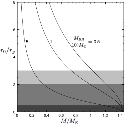
Figure 1: Radius $r_{0}$ where tidal stripping begins, in units of the Schwarzschild radius $r_{g}\equiv 2GM_{\rm BH}/c^{2}\approx 3\times 10^{10}(M_{\rm BH}/10^{5}M_{\odot})$ cm, is shown as a function of the WD mass. The three curves correspond to $M_{\rm BH}/10^{5}M_{\odot}=0.5$, 1 and 5. The value of $r_{0}$ was estimated using the simplified equation (6), which is non-relativistic and neglects the effect of the black-hole spin $a_{s}$ on the tidal force. The shaded region shows radii $r<r_{\min}$ where no stable bound orbits exist. $r_{\min}$ depends on $a_{s}$ and orbital eccentricity $e$, in particular $r_{\min}=3r_{g}$ for $\{a_{s}=0,e=0\}$, $r_{\min}=2r_{g}$ for $\{a_{s}=0,e=1\}$ and $r_{\min}=r_{g}/2$ for $\{a_{s}=1,e=1\}$.

2.2 Estimate for mass loss in one orbital period

As the star begins to lose mass, it continues to do so repeatedly: at each pericenter passage the star overflows the Roche lobe for a short time. The hydrodynamics of the surface layers of the tidally stripped star is complicated. It is clear however that the mass lost in one pericenter passage, $\delta M$, will be tiny for the initial mass loss episodes when the star surface barely touches the Roche lobe. The natural small parameter in the problem is $\Delta/R=(R-R_{t})/R$. The onset of mass loss is defined by $\Delta=0$ and we assume that the dependence of $\delta M$ on $\Delta/R\ll 1$ can be expanded in series whose leading term has the form,

$$\frac{\delta M}{M}=A\,\left(\frac{\Delta}{R}\right)^{\psi},\qquad\Delta\equiv R-R_{t}\ll R,$$ (7)

where $A$ is a numerical factor.

For illustration, consider a toy model. Suppose that after the pericenter passage the star loses the surface shell $\Delta\ll R$ whose mass is estimated using the structure of the unperturbed star,

$$\delta M=4\pi R^{2}\int_{0}^{\Delta}\rho(z)\,dz.$$ (8)

Here $z$ is the depth measured inward from the surface, and $\rho(z)$ is the mass density of the unperturbed star at depth $z$. For simplicity, let us assume the polytropic equation of state in the surface layer $P=K\rho^{\gamma}$ with $\gamma=5/3$, the same as in the deeper region where electrons become degenerate. $P$ and $\rho$ change continuously between the degenerate and non-degenerate regions, and therefore $K$ in the surface layers must be the same as for non-relativistic degenerate electron gas,

$$K\equiv\frac{1}{20}\left(\frac{3}{\pi}\right)^{2/3}\frac{h^{2}}{m_{e}(\mu_{e}m_{p})^{5/3}},$$ (9)

where $\mu_{e}\approx 2$ is the mean molecular weight per electron. The hydrostatic balance $dP/dz=\rho\,GM/R^{2}$ gives

$$\rho(z)=\left(\frac{2GM}{5KR}\right)^{3/2}\left(\frac{z}{R}\right)^{3/2},$$ (10)

and evaluating the integral in equation (8) one finds $\delta M/M=A(\Delta/R)^{\psi}$ with

$$\psi=\frac{5}{2},\qquad A\approx 6.1\left(1-\frac{M}{M_{\rm Ch}}\right)^{3\beta/2}.$$ (11)

In this toy model, $\delta M=(6/5)[\rho(\Delta)/\bar{\rho}](\Delta/R)$ where $\bar{\rho}=3M/4\pi R^{3}$. The small factor $(\Delta/R)^{\psi}\ll 1$ in $\delta M$ results from the small thickness of the surface layer $\Delta$ and the small density of this layer, $\rho(\Delta)/\bar{\rho}\sim(\Delta/R)^{3/2}$.

Additional factors may enter a more realistic model. The duration of the mass-loss episode $\delta t$ may be so short that only a fraction of the $\Delta$-layer is lost. $\delta t$ likely scales with some power of $\Delta/R$. One could formulate a time-dependent model for the mass-loss episode by evaluating $R_{t}$ along the orbit around the pericenter (instead of just one point $r_{p}$). If one assumes that the mass-loss episode occurs where $R_{t}<R$, then $\delta t\sim(\Delta/R)^{1/2}\tau$ where $\tau$ is the sound-crossing time of the star. A complete hydrodynamical model is three-dimensional as the mass loss is asymmetric: gas will flow through the $L_{1}$ point, as happens in close binary systems. The flow velocity may be comparable to the sound speed in the outer layers of the star (which is smaller than the sound speed in its interior). Perhaps future hydrodynamical calculations will give the duration of the mass loss episode and the resulting $\psi$, $A$ and $\delta M$. We do not know the exact values of $\psi$ and $A$ and keep them as parameters. The illustrative numerical example shown below assumes $\psi$ and $A$ given in equation (11).

From equations (4) and (6) one finds

$$\frac{\Delta}{R}=1-\frac{R_{t}}{R}=1-\frac{r_{p}}{r_{0}}\left(\frac{M}{M_{0}}\right)^{2/3}\left(\frac{M_{\rm Ch}-M_{0}}{M_{\rm Ch}-M}\right)^{\beta}.$$ (12)

For the first mass loss episode, $M=M_{0}$ and $r_{p}/r_{0}\sim 1-\alpha$, which implies $\Delta/R\sim\alpha\sim 10^{-5}$. Equation (12) shows that $\Delta$ grows with each passage of the pericenter as $r_{p}$ decreases (due to gravitational radiation) and $M$ decreases (due to mass loss).

2.3 Evolution of mass loss over many orbits

$N$ orbits after the star reached $r_{0}$, the pericenter radius is given by

$$\frac{r_{p}}{r_{0}}\approx 1-\alpha N,\qquad\alpha N\ll 1,$$ (13)

where $\alpha$ is given by equation (3). Here we assumed that $r_{p}$ decreases by $\alpha r_{p}$ in each orbit, neglecting the effect of mass loss on the orbit (which is likely to be a poor approximation at late stages of mass loss, e.g. Bildsten & Cutler 1992).

Let $x$ be the mass fraction of the star that has been lost over $N$ orbits,

$$x=\frac{M_{0}-M}{M_{0}}.$$ (14)

As long as $x\ll 1$, one can expand $\Delta$ in $x$ and $\alpha N$ and keep only the leading linear terms,

$$\frac{\Delta}{R}\approx\frac{\Delta}{R_{0}}\approx\alpha\,N+B\,x,\qquad B=\frac{2}{3}+\frac{\beta M_{0}}{M_{\rm Ch}-M_{0}}.$$ (15)

The term $\alpha N$ describes the change in $R_{t}/R_{0}$ due to the decreasing $r_{p}$ while the small changes in $M$ and $R$ are neglected. The term $Bx$ describes the effect of decreasing $M$ on $R_{t}$ and $R$ while the small drift of the pericenter is neglected.

It is convenient to treat $N\gg 1$ as a continuous variable and describe the mass loss by the differential equation $dM/dN=-\delta M$. Then substitution of equation (15) to equation (7) gives the differential equation for $x(N)$,

$$\frac{dx}{dN}=A\left(\alpha N+Bx\right)^{\psi}.$$ (16)

One can see from this equation that there are two stages of mass loss: (a) $Bx\ll\alpha N$ and (b) $Bx\gg\alpha N$. Assuming $\psi>1$, we find the solutions for the two regimes,

$$x\approx\frac{A}{\psi+1}\,\alpha^{\psi}N^{\psi+1},\qquad N<N_{1},$$ (17)

$$x\approx\left[(\psi-1)AB^{\psi}(N_{\star}-N)\right]^{1/(1-\psi)},\qquad N>N_{1}.$$ (18)

Equation (18) applies only as long as $x\ll 1$, however it gives an estimate for the number of orbits to complete disruption $N_{\star}$. The values of $N_{1}$ and $N_{\star}$ can be evaluated by matching $x$ and $dx/dN$ for the two solutions at $N=N_{1}$,

$$N_{1}=\left(\frac{\psi+1}{AB}\right)^{1/\psi}\alpha^{(1-\psi)/\psi},$$ (19)

$$\frac{N_{\star}-N_{1}}{N_{1}}=\frac{1}{\psi^{2}-1}.$$ (20)

At $N<N_{1}$ the growth of $x$ is caused by the decrease in $r_{p}$ at practically unchanged mass and radius of the star. After $N_{1}$ orbits, the growth of $x$ accelerates as it is now controlled by the decreasing $M$ (and increasing $R$) while the change in $r_{p}$ has a negligible effect. Equations (17) and (18) imply that $\delta M\propto N^{\psi}$ for $N<N_{1}$ and $\delta M\propto(N_{\star}-N)^{\psi/(1-\psi)}$ for $N>N_{1}$.

For example, consider the toy model described by equation (11). In this case, $N_{1}\sim\alpha^{-3/5}\sim 10^{3}$ and $N_{\star}-N_{1}=(4/21)N_{1}$. The mass fraction lost after $N_{1}$ orbits is $x(N_{1})\sim\alpha N_{1}/B\sim\alpha^{2/5}\sim 10^{-2}$. The detailed behavior of $x(N)$ in the toy model is shown in Figure 2 for a WD with initial mass $M_{0}=0.6M_{\odot}$. The figure shows the solution of equation $dx/dN=A(\Delta/R)^{\psi}$ with $\Delta$ given by equation (12).

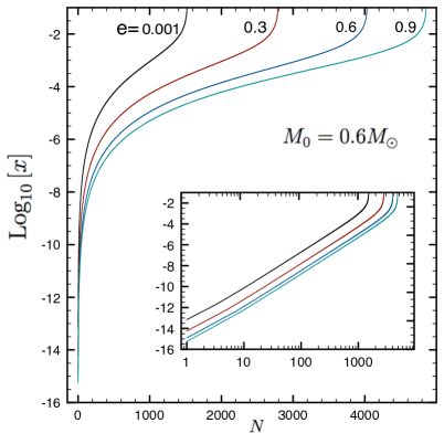
Figure 2: Lost mass fraction $x=(M_{0}-M)/M_{0}$ after $N$ orbits since the onset of tidal stripping. The WD has initial mass $M_{0}=0.6M_{\odot}$. Different curves correspond to different eccentricities of the orbit; $M_{\rm BH}=10^{5}M_{\odot}$ is assumed for all cases. The insert shows $\log x$ plotted against $\log N$.

2.4 Periodic mass-loss rate

The mass-loss rate $dM/dt$ is nearly periodic with the orbital period $P$. It is zero throughout most of the orbit and has a strong peak near the pericenter. To illustrate this behavior, we calculated the following, greatly simplified model,

$$\frac{dM}{dt}=\left\{\begin{array}[]{ll}-\delta M/\tau(M)&R_{t}<R\\ 0&R_{t}>R\end{array}\right.$$ (23)

where $R(M)$ is the radius of the unperturbed star of mass $M$, $R_{t}$ is calculated everywhere along the orbit according to equation (4). $\delta M(t)$ is given by equation (7) (it is evaluated using the local value of $R_{t}$); $\tau=(G\bar{\rho})^{-1/2}$ is the sound-crossing time-scale of the star.

Figure 3 shows the numerical solution of equation (23) for the last 35 orbits before disruption. The WD is assumed to have an initial mass $M_{0}=0.6M_{\odot}$ and orbital eccentricity $e=0.9$; the orbital period is $P\approx 2\times 10^{3}$ s. We plot the instantaneous mass-loss rate $|dM/dt|$ versus time $t_{\rm loss}$ shown by a clock that ticks only when $dM/dt\neq 0$. The periodic peaks in $|dM/dt|$ coincide with the pericenter passages.

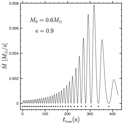
Figure 3: Instantaneous mass-loss rate $\dot{M}=|dM/dt|$ during the last 35 orbits before disruption. The WD with initial mass $M_{0}=0.6M_{\odot}$ is orbiting a black hole with $M_{\rm BH}=10^{5}M_{\odot}$; the orbit has eccentricity $e=0.9$. The horizontal axis shows ‘time during mass transfer’, which increases only when $\dot{M}\neq 0$. The area under each peak is the mass lost per pericenter passage; it follows a power law with the number of orbits left to complete disruption, $\delta M\propto(N_{\star}-N)^{-1.8}$, close to the results of Section 2.3.

3 Discussion: electromagnetic counterpart

The standard picture of EMRI envisions an orbit that gradually shrinks due to gravitational radiation until its pericenter $r_{p}$ reaches $r_{\min}$ where the orbit becomes unstable and plunges into the black hole. The main observational phase of the inspiral is when $r_{p}$ decreases from $\sim 2r_{\min}$ to $r_{\min}$. For WDs with mass $M\sim M_{\odot}$ inspiraling into a black hole with $M_{\rm BH}\sim 10^{5}M_{\odot}$ the main observational phase lasts $\sim 10^{5}$ orbital periods, which may be comparable to one year, depending on the orbital eccentricity. We argued in Section 2 that the inspiraling WDs can experience an extended period of slow mass loss during observations by LISA.

To summarize, the tidal stripping begins very gently because the pericenter of the orbit drifts inward slowly, by a tiny fraction $\alpha\sim 10^{-5}$ in one orbital period. This leads to many repeated episodes of small mass loss. The process occurs at radius $r_{0}$ (eq. 6), comparable to $r_{\min}$. The star is strongly deformed by the tidal forces near $r_{0}$ but it barely touches its Roche lobe for a small fraction of the orbital period. As a result, the star loses a small amount of mass through the $L_{1}$ point at each pericenter passage. To our knowledge, this regime of tidal stripping was not explored by direct hydrodynamical simulations. Our crude estimates suggest two phases of stripping: the first phase lasts $N_{1}\sim 10^{3}$ orbits until the star loses $\sim 1$ per cent of its mass. Then the mass loss accelerates: the decrease in $M$ (and the corresponding increase in the WD radius) implies that the star overfills the Roche lobe more and more with every pericenter passage. As a result, the star loses the remaining 99 per cent of its mass in a few hundreds of additional orbits. The mass lost in each individual episode during these last hundreds of orbits behaves as $\delta M\propto(N_{\star}-N)^{-\xi}$ where $N_{\star}-N\ll N_{\star}$ is the number of orbits remaining to complete disruption and $\xi\sim\psi/(\psi-1)$.

According to our estimates, tidal stripping operates for days or weeks, creating a relatively long-lived source of gas. The gas can accrete onto the black hole and produce significant electromagnetic radiation together with the gravitational waves observed by LISA. The radiation source may become bright before the mass loss spoils the standard EMRI template for the gravitational-wave signal.

The gas produced by tidal stripping moves on nearly Keplerian orbits that are initially close to the WD orbit. The gas probably leaves the star with relative velocity $\sim v_{\rm esc}=(2GM/R)^{1/2}$ and its orbital energy differs from that of the star by a small fraction $\sim v_{\rm esc}/v\sim(Mr_{0}/M_{\rm BH}R)^{1/2}\sim\gamma^{-1/2}(M/M_{\rm BH})^{1/3}\sim 1/30$. After $\sim 30$ orbital periods, the differential rotation of the gas has stretched it into a ring around the black hole. A non-zero eccentricity of the donor orbit will create an eccentric ring. It should viscously spread and accrete onto the black hole. A small mass-loss fraction $x$ can be a huge source of gas for accretion. If most of the stripped matter is accreted by the black hole, the accretion rate is $\dot{M}\sim\delta M/P$. It exceeds the Eddington value $\dot{M}_{\rm Edd}\sim 10^{23}(M_{\rm BH}/10^{5}M_{\odot})$ g s^-1 after $N\sim 10$ orbits since the beginning of tidal stripping, well before the final disruption of the WD. The accretion timescale in the viscous ring can be estimated as $t_{\rm acc}\sim\alpha_{v}^{-1}(H/r)^{-2}P$ where $P$ is the WD orbital period, $\alpha_{v}=0.01-0.1$ is the viscosity parameter and $H$ is the thickness of the ring (e.g. Shakura & Sunyaev 1973). $H/r\sim 1$ is expected for super-Eddington accretion, which leads to $t_{\rm acc}\sim(10-100)P$.

This suggests that a bright source with Eddington luminosity $L_{\rm Edd}\sim 10^{43}$ erg s^-1 is created quickly, in less than 1 day after the beginning of tidal stripping. For a typical distance to such LISA sources, $d\sim 100$ Mpc, the accretion ring should be detectable with optical and X-ray telescopes provided its approximate location on the sky is known. LISA is expected to localize EMRIs within $\sim 10$ deg² (Barack & Cutler 2004). For massive black-hole mergers, the localization information will be available weeks to months prior to the final coalescence (Kocsis et al. 2007, 2008; Lang & Hughes 2008), and the localization expectations for WD EMRIs are similar (S. Drasco, J. Gair, I. Mandel, E. Porter, private communications), giving sufficient time for simultaneous optical and X-ray observations during inspiral.

Mass transfer in WD inspirals is special as it creates a long-lived source of gas very close to the black hole horizon, $r_{0}-r_{g}\sim r_{g}$. As a result, the donor orbit is generally not confined to a plane, if the black hole rotation is significant. Besides, the orbit will experience fast precession. Therefore, the freshly stripped gas may collide with the previously released gas and generate shocks (e.g. Evans & Kochanek 1989). The resulting pattern of accretion may be complicated and needs careful study.

An intriguing feature of tidal stripping is the periodic supply of gas. It may leave a fingerprint on the observed luminosity, modulating it with the WD orbital period $P$. The modulation of $\dot{M}$ may create a detectable oscillation in the luminosity from the accreting ring, even though the accretion timescale $t_{\rm acc}\sim(10-100)P\gg P$, tends to reduce the amplitude of modulation. The shock emission from collisions between the periodic flow from the $L_{1}$ point and the gas accumulated around the black hole may be strongly modulated.

The description of mass transfer in this paper is greatly simplified. The possibility of many repeated mass-transfer episodes is robust, but the exact rate of tidal stripping and the dynamics of accretion need to be explored with dedicated numerical simulations. The great potential that such events hold for joint detections of gravitational and electromagnetic radiation provides motivation for the effort. The joint detection would let us witness, in real-time and unprecedented detail, the slow tidal stripping of a WD followed by its complete disruption. Note that LISA observations are expected to provide the mass and spin of the black hole, as well as the details of the inspiral orbit. This can be used to model in detail the hydrodynamics of accretion.

The scenario discussed in this paper assumes $r_{0}>r_{\min}$ and uses a semi-Newtonian description for the WD orbit. A fully relativistic model will be needed to accurately evaluate the parameter space for such events. The relativistic effects are especially important if the black hole is rapidly rotating – then $r_{0}$ and $r_{\min}$ will depend on the black hole mass $M_{\rm BH}$, its spin parameter $a_{s}$, the eccentricity of the orbit, and the angle between the orbital angular momentum and the angular momentum of the black hole. The competition between tidal disruption and gravitational capture by rotating black holes was investigated for parabolic orbits in Beloborodov et al. (1992). In a broad range of $M_{\rm BH}$, the fate of a star approaching the black hole depends on the orbit orientation and can be either disruption or capture. For inspirals with $r_{g}<r_{0}<r_{\min}$, tidal stripping does not occur. Instead, $r_{p}$ reaches $r_{\min}$ and the orbit loses stability before any mass is lost by the WD. Then the star is crushed by tidal forces as it falls into the black hole. This strong and immediate disruption is different from the gentle stripping considered here, suggesting rich phenomenology of WD inspirals.

References

- Bildsten (1992) Bildsten L., Cutler C., 1992, ApJ, 400, 175
- Barack (2004) Barack L., Cutler C., 2004, Phys. Rev. D, 69, 082005
- B (1992) Beloborodov A. M., Illarionov A. F., Ivanov P. B., Polnarev A. G., 1992, MNRAS, 259, 209
- Bloom (2009) Bloom J. S., Holz D. E., Hughes S. A., Menou K., 2009, Astro2010 Science White Papers, no. 20 (arXiv:0902.1527)
- Cutler (1998) Cutler C., 1998, Phys. Rev. D, 57, 7080
- Evans et. al. (1989) Evans C. R., Kochanek C. S., 1989, ApJ, 346, L13
- Freitag (2003) Freitag M., 2003, ApJ, 583, L21
- Gair et. al. (2004) Gair J. R. et al., 2004, Class. Quant. Grav., 20, S1595
- Hils et al. (1995) Hils D., Bender P. L., 1995, ApJ, 445, L7
- Hopman (2009) Hopman C., 2009, Class. Quant. Grav., 26, 094028
- Hopman et al. (2005) Hopman C., Alexander T., 2005, ApJ, 629, 362
- Hopman et al. (2006a) Hopman C., Alexander T., 2006a, ApJ, 645, L133
- Hopman et al. (2006b) Hopman C., Alexander T., 2006b, ApJ, 645, 1152
- Hughes (2009) Hughes S. A., 2009, ARA& A, 47, 107
- Ivanov (2002) Ivanov P. B., 2002, MNRAS, 336, 373
- Ivanov et al. (2007) Ivanov P. B., Papaloizou J. C. B., 2007, A& A, 476, 121
- Kobayashi et al. (2004) Kobayashi S., Laguna P., Phinney E. S., Meszaros P., 2004, ApJ, 615, 855
- Kocsis et al. (2007) Kocsis B., Haiman Z., Menou K., Frei Z., 2007, Phys. Rev. D, 76, 022003
- Kocsis et al. (2008) Kocsis B., Haiman Z., Menou K., 2008, ApJ, 684, 870
- Lang et al. (2008) Lang R. N., Hughes S. A., 2008, ApJ, 677, 1184
- Menou et al. (2008) Menou K., Haiman Z., Kocsis B., 2008, NewAR, 51, 884
- Miller et al. (2005) Miller, M. C., Freitag, M., Hamilton, D. P. & Lauburg, V. M. 2005, ApJ, 631, L117
- Peters (1964) Peters P. C., 1964, Phys. Rev., 136, B 1224
- Phinney (2009) Phinney E. S., 2009, Astro2010 Science White Papers, no. 235 (arXiv:0903.0098)
- Rathore et. al. (2005) Rathore Y., Blandford R. D., Broderick A. E., 2005, MNRAS, 357, 834
- Ritter (1988) Ritter H., 1988, A&A, 202, 93
- Rosswog et. al. (2009) Rosswog S., Ramirez-Ruiz E., Hix W. R., 2009, ApJ, 695, 404
- Sathyaprakash (2009) Sathyaprakash B. S., Schutz B. F., 2009, Liv. Rev. Rel., 12, 2
- Sepinsky (2007) Sepinsky J. F., Willems B., Kalogera V., 2007, ApJ, 660, 1624
- Sesana (2008) Sesana A., Vecchio A., Eracleous M., Sigurdsson S., 2008, MNRAS, 391, 718
- Shakura (1973) Shakura N. I., Sunyaev R. A., 1973, A&A, 24, 337
- Sigurdsson et. al. (1997) Sigurdsson S., Rees M. J., 1997, MNRAS, 284, 318