The Gauge Bosons Masses in a $SU(2)_{TC}\otimes SU(3)_{{}_{L}}\otimes U(1)_{{}_{X}}$ Extension of the Standard Model

Abstract

The gauge symmetry breaking in 3-3-1 models can be implemented dynamically because at the scale of a few TeVs the $U(1)_{X}$ coupling constant becomes strong. The exotic quark $T$ introduced in the model will form a condensate breaking $SU(3)_{{}_{L}}\otimes U(1)_{X}$ to electroweak symmetry. In this brief report we explore the full realization of the dynamical symmetry breaking of an 3-3-1 model to $U(1)_{em}$ considering a model based on $SU(2)_{TC}\otimes SU(3)_{{}_{L}}\otimes U(1)_{{}_{X}}$. We compute the mass generated for the charged and neutral gauge bosons of the model that result from the symmetry breaking, and verify the equivalence between a 3-3-1 model with a scalar content formed by the set of the fundamental scalar bosons $\chi,\rho$ and $\eta$ with a 3-3-1 model where the dynamical symmetry breaking is implanted by the system formed by the set of composite bosons $\Phi_{{}_{T}},\Phi_{{}_{TC(1)}}$ and $\Phi_{{}_{TC(2)}}$. In this model the minimal composite scalar content is fixed by the condition of the cancellation of triangular anomaly in TC sector.

The Standard Model of elementary particles is in excellent agreement with the experimental data and has explained many features of particle physics throughout the years. Despite its success, there are some points in the model that could be better explained with the introduction of new fields and symmetries, such as the flavor problem or the enormous range of masses between the lightest and heaviest fermions and other peculiarities. One of the possibilities in this direction is to assume an extension of the standard model based on $G_{3n1}\equiv SU(3)_{{}_{C}}\otimes SU(n)_{{}_{L}}\otimes U(1)_{{}_{X}}$felice1 ; frampton ; tonasse ; felice2 , where $n=3,4$. This class of the models predicts interesting new physics at TeV scaletrecentes and addresses some fundamental questions that cannot be explained in the framework of the Standard Model. As a brief example we can mention the flavor problemdp1 and the question of the electric charge quantizationdp2 .

One interesting feature of some versions of these models is the following relationship among the coupling constants $g$ and $g^{\prime}$ associated to the gauge group $SU(3)_{{}_{L}}\otimes U(1)_{{}_{X}}$

$$\frac{\alpha^{\prime}}{\alpha}=\frac{\sin^{2}\theta_{{}_{W}}(\mu)}{1-4\sin^{2}\theta_{{}_{W}}(\mu)}$$ (1)

where $\alpha=g^{2}/4\pi$, $\alpha^{\prime}=g^{\prime 2}/4\pi$ and $\theta{{}_{W}}$ is the electroweak mixing angle. As argued in Refs.Das ; doff , the gauge symmetry breaking of $SU(3)_{{}_{L}}\otimes U(1)_{{}_{X}}$ in 3-3-1 models can be implemented dynamically because at the scale of a few TeVs, $\mu_{X}$, the $U(1)_{X}$ coupling constant $(g^{\prime})$ becomes strong as we approach the peak existent in Eq.(1). The exotic quark $J_{3}$ introduced in these models, in our notation $J_{3}\equiv T$ , will form a condensate breaking $SU(3)_{{}_{L}}\otimes U(1)_{{}_{X}}$ to electroweak gauge symmetry without requiring the introduction of fundamental scalars. In Ref.doff we investigated this possibility and show that just versiontonasse of this class of models leads to a deeper minimum of the effective potential.

The mechanism that breaks the electroweak symmetry $SU(2)_{{}_{L}}\otimes U(1)_{{}_{Y}}$ down to the gauge symmetry of electromagnetism $U(1)_{em}$ is still the only obscure part of the standard model and the understanding of the gauge electroweak symmetry breaking mechanism is one of the most important problems in particle physics at present. One of the explanations of this mechanism is based on the introduction of a new strong interaction usually named technicolor (TC), where in these theories the Higgs boson is a composite of the so called technifermions. The beautiful characteristics of technicolor (TC) as well as its problems are clearly described in Refs.lane ; simmons .

In this work we will extend the results obtained in doff , in particular, we intend to explore the full realization of the dynamical symmetry breaking of modeltonasse to $U(1)_{em}$ considering $SU(2)_{TC}\otimes SU(3)_{{}_{L}}\otimes U(1)_{{}_{X}}$ group, where $SU(2)_{TC}$ is the minimal TC gauge group that will be responsible for the electroweak symmetry breaking.

We begin determining the mass generated for the charged gauge bosons of the model that results from the symmetry breaking assuming the charged current interactions associated to the technifermions and to the exotic quark T, that will be responsible for the mass generation of the heavy gauge bosons $V^{\pm}$ and $U^{\pm\pm}$. In the sequence we obtain the neutral current interactions and the mass matrix generated for the neutral gauge bosons.

The fermionic content of the model has the same quark sector of Ref.felice1

$$Q_{3L}=\left(\begin{array}[]{c}t\\ b\\ T\end{array}\right)_{L}\,\,\sim\,\,({\bf 1},{\bf 3},2/3)$$ (5)

$$t_{R}\,\sim\,({\bf 1},{\bf 1},2/3)\,,\,b_{R}\,\sim\,({\bf 1},{\bf 1},-1/3)$$

$$T_{R}\,\sim\,({\bf 1},{\bf 1},5/3)$$

$$Q_{\alpha L}=\left(\begin{array}[]{c}D\\ u\\ d\end{array}\right)_{\alpha L}\,\,\sim\,\,({\bf 1},{\bf 3^{*}},-1/3)$$ (9)

$$u_{\alpha R}\,\sim\,({\bf 1},{\bf 1},2/3)\,,\,d_{\alpha R}\,\sim\,({\bf 1},{\bf 1},-1/3)$$

$$D_{\alpha R}\,\sim\,({\bf 1},{\bf 1},-4/3)$$ (10)

where $\alpha=1,2$ is the family index and we represent the third quark family by $Q_{3L}$. In these expressions $({\bf 1},{\bf 3},X)$, $({\bf 1},{\bf 3^{*}},X)$ or $({\bf 1},{\bf 1},X)$ denote the transformation properties under $SU(2)_{TC}\otimes SU(3)_{{}_{L}}\otimes U(1)_{{}_{X}}$ and $X$ is the corresponding $U(1)_{X}$ charge. The leptonic sector includes beside the conventional charged leptons and their respective neutrinos, charged heavy leptons $E_{a}$tonasse .

$$l_{aL}=\left(\begin{array}[]{c}\nu_{a}\\ l_{a}\\ E^{c}_{a}\end{array}\right)_{L}\,\sim\,({\bf 1},{\bf 3},0)$$ (14)

where $a=1,2,3$ is the family index and $l_{aL}$ transforms as triplets under $SU(3)_{L}$. Moreover, we have to add the corresponding right-handed components, $l_{aR}\sim({\bf 1},{\bf 1},-1)$ and $E^{c}_{aR}\sim({\bf 1},{\bf 1},+1)$.

In addition, we included the minimal Technicolor sector, represented by

$$\Psi_{1L}=\left(\begin{array}[]{c}U_{1}\\ D_{1}\\ U^{\prime}\end{array}\right)_{L}\,\,\sim\,\,({\bf 2},{\bf 3},1/2)$$ (18)

$$U_{1R}\,\sim\,({\bf 2},{\bf 1},1/2)\,,\,D_{1R}\,\sim\,({\bf 2},{\bf 1},-1/2)$$

$$U^{\prime}_{R}\,\sim\,({\bf 2},{\bf 1},3/2),$$

$$\Psi_{2L}=\left(\begin{array}[]{c}D^{\prime}\\ U_{2}\\ D_{2}\end{array}\right)_{L}\,\,\sim\,\,({\bf 2},{\bf 3^{*}},-1/2)$$ (22)

$$U_{2R}\,\sim\,({\bf 2},{\bf 1},1/2)\,,\,D_{2R}\,\sim\,({\bf 2},{\bf 1},-1/2)$$

$$D^{\prime}_{R}\,\sim\,({\bf 2},{\bf 1},-3/2).$$ (23)

where $1$ and $2$ label the first and second techniquark families, $U^{\prime}$ and $D^{\prime}$ can be considered as exotic techniquarks making an analogy with quarks $T$ and $D$ that appear in the fermionic content of the model . The model is anomaly free if we have equal numbers of triplets and antitriplets, counting the color of $SU(3)_{c}$. Therefore, in order to make the model anomaly free two of the three quark generations transform as ${\bf 3^{*}}$, the third quark family and the three leptons generations transform as ${\bf 3}$. It is easy to check that all gauge anomalies cancel out in this model, in the TC sector the triangular anomaly cancels between the two generations of technifermions. In the present version of the model we assumed that technifermions are singlets of $SU(3)_{c}$.

The charged current interactions with the quark $T$ are described by

$${\cal L}^{cc}_{Q_{3L}}=\frac{g}{\sqrt{2}}\left(\bar{T}_{L}\gamma^{\mu}t_{L}V^{+}_{\mu}+\bar{T}_{L}\gamma^{\mu}b_{L}U^{++}_{\mu}+h.c.\right)$$ (24)

For the TC sector, the charged current interactions to the first technifermion generation can be written as

$${\cal L}^{cc}_{TC(1)}=\frac{g}{\sqrt{2}} \left(\bar{U}_{1L}\gamma^{\mu}D_{1L}W^{+}_{\mu}+\bar{U^{\prime}}_{L}\gamma^{\mu}U_{1L}V^{+}_{\mu}+\right.$$ (25)

$$\left.\bar{U^{\prime}}_{L}\gamma^{\mu}D_{1L}U^{++}_{\mu}+h.c.\right),$$

while for the second technifermion generation we obtain

$${\cal L}^{cc}_{TC(2)}=\frac{g}{\sqrt{2}} \left(\bar{U}_{2L}\gamma^{\mu}D_{2L}W^{+}_{\mu}+\bar{D}_{2L}\gamma^{\mu}D^{\prime}_{L}V^{+}_{\mu}+\right.$$ (26)

$$\left.\bar{U}_{2L}\gamma^{\mu}D^{\prime}_{L}U^{++}_{\mu}+h.c.\right).$$

From these, we can extract the couplings of charged gauge bosons with the axial currents $J^{\mu}_{5(T)}=\frac{1}{2}\bar{T}\gamma^{\mu}\gamma_{5}\Psi_{i}$, with $\Psi_{i}=t,b$, $J^{\mu}_{5(1)}=\frac{1}{2}\bar{U_{1}}\gamma^{\mu}\gamma_{5}D_{1}$, $J^{\mu}_{5(1^{\prime})}=\frac{1}{2}\bar{U^{\prime}}\gamma^{\mu}\gamma_{5}\Psi_{j}$ where $\Psi_{j}=U_{1},D_{1}$, and $J^{\mu}_{5(2)}=\frac{1}{2}\bar{U_{2}}\gamma^{\mu}\gamma_{5}D_{2}$ , $J^{\mu}_{5(2^{\prime})}=\frac{1}{2}\bar{\Psi_{k}}\gamma^{\mu}\gamma_{5}D^{\prime}$ to $\Psi_{k}=D_{2},U_{2}$. After considering the decay constant relations for the axial currents

$$\langle 0|J^{\mu}_{5(T)}|\Pi\rangle\sim i\frac{F_{\Pi}}{\sqrt{2}}p^{\mu}$$

$$\langle 0|J^{\mu}_{5(1,1^{\prime})}|\pi_{1}\rangle\sim i\frac{f_{\pi_{1}}}{\sqrt{2}}p^{\mu}\,,\,\langle 0|J^{\mu}_{5(2,2^{\prime})}|\pi_{2}\rangle\sim i\frac{f_{\pi_{2}}}{\sqrt{2}}p^{\mu}$$ (27)

we can write the interaction terms of the charged bosons $V^{\pm}$, $U^{\pm\pm}$ and $W^{\pm}$ with $U(1)_{X}$ and TC pions $(\Pi,\pi_{1},\pi_{2})$ as

$${\cal L}_{\Pi-V}=-\frac{ig}{2}F_{\Pi}p^{\mu}V^{\pm}_{\mu}\,\,,\,\,{\cal L}_{\pi-V}=-\frac{ig}{2}\left[f_{\pi_{1}}p^{\mu}+f_{\pi_{2}}p^{\mu}\right]V^{\pm}_{\mu}$$

$${\cal L}_{\Pi-U}=-\frac{ig}{2}F_{\Pi}p^{\mu}U^{\pm\pm}_{\mu}\!\!\!\!\,\,,\,\,{\cal L}_{\pi-U}=-\frac{ig}{2}\left[f_{\pi_{1}}p^{\mu}+f_{\pi_{2}}p^{\mu}\right]U^{\pm\pm}_{\mu}$$

$${\cal L}_{\pi-W}=-\frac{ig}{2}\left[f_{\pi_{1}}p^{\mu}+f_{\pi_{2}}p^{\mu}\right]W^{\pm}_{\mu}.$$ (28)

In the equations above the technipion decay constants, $(f_{\pi_{1}}=f_{\pi_{1}^{\pm}})$ and $(f_{\pi_{2}}=f_{\pi_{2}^{\pm}})$, are related to the vacuum expectation value(VEV) of the Standard Model through

$$\left(f^{2}_{\pi_{1}}+f^{2}_{\pi_{2}}\right)=v^{2}=\frac{4M_{W}^{2}}{g^{2}}$$ (29)

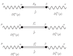
Figure 1: Contributions to the vacuum polarization $\Pi_{\alpha\beta}(p^{2})$ of the charged gauge boson $V^{\pm}$.

and we will consider that $F_{\Pi}\!\sim\!\mu_{X}\!\sim\!O(TeV)$.

Technicolor models with fermions in the fundamental representation are subjected to a strong experimental constraint that comes from the limits on the $S$ parameter. In our case, the contribution due to the TC sector should still lead to a value to the S parameter compatible with the experimental data. At low energies, i.e. at the scale associated with electroweak symmetry breaking, we should only consider the contribution of four techniquarks because (U ’and D’) are singlets of $SU(2)_{L}$ and do not contribute directly to the mass of (W and Z) bosons.

In Fig.I we show the couplings in $O(g^{2})$ between the charged pions, $\Pi^{\pm}$ and $\pi^{\pm}_{1,2}$, with the charged boson $V^{\pm}$. From this figure we can write the correction to the $V^{\pm}$ propagator as

$$iD^{\prime}_{V}(p^{2})^{\mu\nu}\!\!=\!iD_{V}(p^{2})^{\mu\nu}\!+\!i\frac{g^{2}}{2}D_{V}(p^{2})^{\mu\alpha}\!\!\left[i\Pi^{V}_{\alpha\beta}(p^{2})\right]iD_{V}(p^{2})^{\beta\nu}$$

where $D_{V}(p^{2})$ is the tree level propagator in the Landau gauge and $\Pi^{V}_{\alpha\beta}(p^{2})$ is obtained from the pions couplings. Then, after considering $\Pi^{V}_{\alpha\beta}(p^{2})=\left(p^{2}g_{\alpha\beta}-p_{\alpha}p_{\beta}\right)\Pi^{V}(p^{2})$ , $M^{2}_{V}=g^{2}p^{2}\Pi^{V}(p^{2})/2$, the contributions for the polarization tensor depicted in Fig. I, and the first equation listed in (28), we obtain

$$M^{2}_{V}=\frac{g^{2}}{4}\left(F^{2}_{\Pi}+f^{2}_{\pi_{1}}+f^{2}_{\pi_{2}}\right).$$ (30)

The mass generated for the $U$ and $W$ bosons can be obtained in the same way, these results are presented below

$$M^{2}_{U}=\frac{g^{2}}{4}\left(F^{2}_{\Pi}+f^{2}_{\pi_{1}}+f^{2}_{\pi_{2}}\right)\,\,,\,\,M^{2}_{W}=\frac{g^{2}}{4}\left(f^{2}_{\pi_{1}}+f^{2}_{\pi_{2}}\right).$$ (31)

The mass generated for neutral bosons $Z_{0}$ and $Z^{\prime}_{0}$ can be determined in a similar way, below we show the couplings of exotic quark $T$ with $W_{8}$ and $B$

$${\cal L}_{T-B-W^{8}}= +\frac{g}{\sqrt{3}}\bar{T}_{L}\gamma_{\mu}T_{L}W^{\mu}_{8}-\frac{2g^{\prime}}{3}\bar{T}_{L}\gamma_{\mu}T_{L}B^{\mu}$$ (32)

$$-\frac{5g^{\prime}}{3}\bar{T}_{R}\gamma_{\mu}T_{R}B^{\mu}$$

where $(B,W_{3},W_{8})$ are symmetry eigenstates, $B$ is the $U(1)_{X}$ boson and the eigenstates $(W_{3},W_{8})$ are associated to the neutral generators of the $SU(3)_{L}$. For the first technifermion generation $(1^{a}ger)$, the respective couplings are listed below

$${\cal L}^{1^{a}\,ger}_{W^{3},W^{8}}=-\frac{g}{2} \left[\bar{U}_{1L}\gamma_{\mu}U_{1L}\left(W^{\mu}_{3}+\frac{1}{\sqrt{3}}W^{\mu}_{8}\right)+\right.$$ (33)

$$\left.\bar{D}_{1L}\gamma_{\mu}D_{1L}\left(-W^{\mu}_{3}+\frac{1}{\sqrt{3}}W^{\mu}_{8}\right)+\right.$$

$$\left.-\frac{2}{\sqrt{3}}\bar{U^{\prime}}_{L}\gamma_{\mu}U^{\prime}_{L}W^{\mu}_{8}\right]$$

$${\cal L}^{1^{a}\,ger}_{B}=-\frac{g^{\prime}}{2} \left[\bar{U}_{1L}\gamma_{\mu}U_{1L}+\bar{D}_{1L}\gamma_{\mu}D_{1L}+\right.$$

$$\left.\bar{U}_{1R}\gamma_{\mu}U_{1R}-\bar{D}_{1R}\gamma_{\mu}D_{1R}+\right.$$

$$\left.3\bar{U^{\prime}}_{R}\gamma_{\mu}U^{\prime}_{R}+\bar{U^{\prime}}_{L}\gamma_{\mu}U^{\prime}_{L}\right]B^{\mu},$$

while that for the $(2^{a}ger)$ we have

$${\cal L}^{2^{a}\,ger}_{W^{3},W^{8}}=-\frac{g}{2} \left[\bar{U}_{2L}\gamma_{\mu}U_{2L}\left(W^{\mu}_{3}-\frac{1}{\sqrt{3}}W^{\mu}_{8}\right)+\right.$$ (35)

$$\left.\bar{D}_{2L}\gamma_{\mu}D_{2L}\left(-W^{\mu}_{3}-\frac{1}{\sqrt{3}}W^{\mu}_{8}\right)+\right.$$

$$\left.+\frac{2}{\sqrt{3}}\bar{D^{\prime}}_{L}\gamma_{\mu}D^{\prime}_{L}W^{\mu}_{8}\right]$$

$${\cal L}^{2^{a}\,ger}_{B}=\frac{g^{\prime}}{2} \left[\bar{U}_{2L}\gamma_{\mu}U_{2L}+\bar{D}_{2L}\gamma_{\mu}D_{2L}+\right.$$

$$\left.-\bar{U}_{2R}\gamma_{\mu}U_{2R}+\bar{D}_{2R}\gamma_{\mu}D_{2R}+\right.$$

$$\left.+3\bar{D^{\prime}}_{R}\gamma_{\mu}D^{\prime}_{R}+\bar{D^{\prime}}_{L}\gamma_{\mu}D^{\prime}_{L}\right]B^{\mu}.$$

In this case the couplings between the neutral pions, $\Pi^{0}$ and $\pi^{0}_{1,2}$, with $W^{3},W^{8}$ and $B$ are

$$\!\!{\cal L}_{\pi^{0}_{1}-W_{3}}=+i\frac{g}{2}f_{\pi_{1}}p_{\mu}W^{\mu}_{3}\,\,,\,\,{\cal L}_{\pi^{0}_{2}-W_{3}}=+i\frac{g}{2}f_{\pi_{2}}p_{\mu}W^{\mu}_{3}$$

$$\!\!{\cal L}_{\pi^{0}_{1}-B}=-i\frac{g^{\prime}}{2}f_{\pi_{1}}p_{\mu}B^{\mu}\,\,,\,\,{\cal L}_{\pi^{0}_{2}-B}=-i\frac{g^{\prime}}{2}f_{\pi_{2}}p_{\mu}B^{\mu}$$

$$\!\!{\cal L}_{\pi^{0}_{1}-W_{8}}=-i\frac{g}{2}f_{\pi_{1}}p_{\mu}\frac{W^{\mu}_{8}}{\sqrt{3}}\,\,,\,\,{\cal L}_{\pi^{0}_{2}-W_{8}}=-i\frac{g}{2}f_{\pi_{2}}p_{\mu}\frac{W^{\mu}_{8}}{\sqrt{3}}$$

$$\!\!{\cal L}_{\pi^{0}_{1}-B}=-i\frac{g^{\prime}}{2}f_{\pi_{1}}p_{\mu}B^{\mu}\,\,,\,\,{\cal L}_{\pi^{0}_{2}-B}=-i\frac{g^{\prime}}{2}f_{\pi_{2}}p_{\mu}B^{\mu}$$

$$\!\!{\cal L}_{\Pi-W_{8}}=-i\frac{g}{2}(2F_{\Pi})p_{\mu}\frac{W^{\mu}_{8}}{\sqrt{3}}\,\,,\,\,{\cal L}_{\Pi-B}=-i\frac{g^{\prime}}{2}(2F_{\Pi})p_{\mu}B^{\mu}.$$

(37)

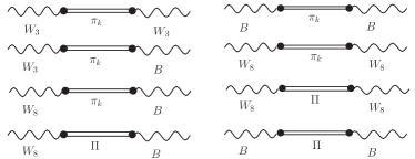
Figure 2: Contributions to the vacuum polarization $\Pi_{\alpha\beta}(p^{2})$ of the neutral gauge bosons. In this figure, $k=1,2$ is the TC family index, and for simplicity we have not written the Lorentz indices.

In Fig. II we represent the contributions of these couplings to the vacuum polarization tensor of the neutral gauge bosons.

Therefore, from the contributions depicted in Fig. II, and after considering Eq.(37), we can write the following mass matrix for neutral bosons in the base $\{W_{3},W_{8},B\}$

$$M^{2}_{neu}=\frac{g^{2}}{4}\left(\begin{array}[]{ccc}A_{W_{3}W_{3}}&0&-A_{W_{3}B}\\ 0&A_{W_{8}W_{8}}&A_{W_{8}B}\\ -A_{BW_{3}}&A_{BW_{8}}&A_{BB}\end{array}\right)$$ (41)

(42)

where

$$A_{W_{3}W_{3}}=f^{2}_{\pi_{1}}+f^{2}_{\pi_{2}}$$

$$A_{BW_{3}}=A_{W_{3}B}=t(f^{2}_{\pi_{1}}+f^{2}_{\pi_{2}})$$

$$A_{W_{8}B}=A_{BW_{8}}=\frac{t}{\sqrt{3}}(f^{2}_{\pi_{1}}+f^{2}_{\pi_{2}})+\frac{4t}{\sqrt{3}}F^{2}_{\Pi}$$

$$A_{W_{8}W_{8}}=\frac{1}{3}(f^{2}_{\pi_{1}}+f^{2}_{\pi_{2}})+\frac{4}{3}F^{2}_{\Pi}$$

$$A_{BB}=2t^{2}(f^{2}_{\pi_{1}}+f^{2}_{\pi_{2}})+4t^{2}F^{2}_{\Pi}.$$ (43)

and we defined $t=\frac{g^{\prime}}{g}$. The eigenvalues of the matrix in Eq.(42), assuming $F_{\Pi}>>f_{\pi_{1}},f_{\pi_{2}}$, are then given by

$$M^{2}_{A}=0\,\,\,\,,\,\,\,M^{2}_{Z_{0}}\simeq\frac{g^{2}}{4}\left(f^{2}_{\pi_{1}}+f^{2}_{\pi_{2}}\right)\left[\frac{1+4t^{2}}{1+3t^{2}}\right]$$

$$M^{2}_{Z^{\prime}_{0}}\simeq\frac{g^{2}}{4}F^{2}_{\Pi}\left[\frac{4}{3}+4t^{2}\right].$$ (44)

The neutral physical states $(A_{\mu},Z_{{0}_{\mu}},Z^{\prime}_{{0}_{\mu}})$ are the same described in Ref.felice1 and $A_{\mu}$ represents the foton field.

In conclusion, the gauge symmetry breaking in 3-3-1 models can be implemented dynamically because at the scale of a few TeVs the $U(1)_{X}$ coupling constant becomes strong as we approach the peak existent in Eq.(1)Das doff . The exotic quark $T$ introduced in model will form a condensate breaking $SU(3)_{{}_{L}}\otimes U(1)_{X}$ to electroweak symmetry. In this work we consider only the T quark contribution to the $U(1)_{X}$ condensate, because we are assuming the most attractive channel(MAC) hypothesisRaby . The MAC should satisfy $\alpha_{c}(\mu_{X})(X_{L}X_{R})\sim 1$, and once $\alpha_{c}(\mu_{X})$ is close to 1, we can roughly estimate that $U(1)_{X}$ condensation should occur only for the channel where $(X_{L}X_{R})\gtrsim 1$. With the exception of the T quark, all other fermions have $(X_{L}X_{R})<1$. A more detailed analysis requires a Schwinger-Dyson equation calculation. However, if contributions due to other channels, such as those associated with $U(1)_{X}$ condensation of D or D’, for example, we expect a mass correction for the exotic gauge bosons(or $F_{\Pi}$) not larger than $20\%$, since $\langle\bar{D}D\rangle\sim O(10^{-1})\langle\bar{T}T\rangle$Das .

In this brief report we explore the full realization of the dynamical symmetry breaking of the $SU(3)_{{}_{L}}\otimes U(1)_{{}_{X}}$ extension of the Standard Modeltonasse considering a model based on $SU(2)_{TC}\otimes SU(3)_{{}_{L}}\otimes U(1)_{{}_{X}}$. The electroweak symmetry is broken dynamically by a technifermion condensate and we have determined the mass generated for the charged gauge bosons of the model that result of the symmetry breaking.

We also determine the mass matrix generated for the neutral gauge bosons of the model and found the same mass spectrum to the gauge bosons obtained with the introduction of fundamental scalars $\chi,\rho$ and $\eta$felice1 tonasse . In other words, we verify the equivalence between a 3-3-1 model with a scalar content formed by $\chi,\rho$ and $\eta$ , with a 3-3-1 model where the dynamical symmetry breaking is implanted by the system formed by the composite scalar bosons $\Phi_{{}_{T}}=(\bar{T}t,\bar{T}b,\bar{T}T)\sim(\phi^{-}_{{}_{T}},\phi^{--}_{{}_{T}},\phi^{0}_{{}_{T}})$, $\Phi_{{}_{TC(1)}}=(\bar{U}_{1}U_{1},\bar{U}_{1}D_{1},\bar{U}_{1}U^{\prime})\sim(\phi^{0}_{{}_{TC(1)}},\phi^{-}_{{}_{TC(1)}},\phi^{+}_{{}_{TC(1)}})$ and $\Phi_{{}_{TC(2)}}=(\bar{D}_{2}U_{2},\bar{D}_{2}D_{2},\bar{D^{\prime}}U_{2})\sim(\phi^{+}_{{}_{TC(2)}},\phi^{0}_{{}_{TC(2)}},\phi^{++}_{{}_{TC(2)}})$. This system of composite bosons will produce the following hierarchical symmetry breaking $SU(3)_{{}_{L}}\otimes U(1)_{{}_{X}}\stackrel{{\scriptstyle a}}{{\longrightarrow}}SU(2)_{{}_{L}}\otimes U(1)_{{}_{Y}}\stackrel{{\scriptstyle b}}{{\longrightarrow}}U_{em}$, with $a=\langle\phi^{0}_{{}_{T}}\rangle$ and $b=\langle\phi^{0}_{{}_{TC(1)}},\phi^{0}_{{}_{TC(2)}}\rangle$. The novelty in this approach is that the minimal scalar content is fixed by the condition of the cancellation of triangular anomaly in TC sector. In Ref.dn we discuss a mechanism for the dynamical mass generation in grand unified models with a horizontal symmetry, incorporating quarks and techniquarks and including the generation of a large t quark mass. We expect that a mechanism similar to the one described in dn can be developed for the model discussed here, this possibility and the determination of the mass spectrum of the composite Higgs bosons are topics that we intend to address in future work.

References

• (1) F. Pisano and V. Pleitez, Phys. Rev. D46, 410 (1992).
• (2) P. H. Frampton, Phys. Rev. Lett. 69, 2889 (1992).
• (3) V. Pleitez and M.D. Tonasse, Phys. Rev. D48, 2353 (1993).
• (4) F. Pisano and V. Pleitez, Phys. Rev. D51 , 3865 (1995).
• (5) Alex G. Dias, C.A. de S.Pires and P.S. Rodrigues da Silva, Phys. Lett. B628, 85 (2005); Alex G. Dias, C.A. de S.Pires, V. Pleitez and P.S. Rodrigues da Silva, Phys. Lett. B621, 151 (2005); Alex G. Dias, A. Doff, C. A. de S. Pires and P.S. Rodrigues da Silva, Phys. Rev. D72, 035006 (2005); Alex Gomes Dias, Phys. Rev. D71, 015009 (2005); Alex G. Dias, J.C. Montero and V. Pleitez, Phys. Lett. B637, 85 (2006); Alex G. Dias and V. Pleitez, Phys. Rev. D73, 017701 (2006), A. Doff, C. A. de S. Pires and P. S. Rodrigues da Silva, Phys. Rev. D74, 015014 (2006).
• (6) A. Doff and F. Pisano, Mod. Phys. Lett. A15, 1471 (2000).
• (7) C.A de S. Pires and O. P. Ravinez, Phys. Rev. D58, 035008 (1998); A. Doff and F. Pisano, Mod. Phys. Lett. A14, 1133 (1999); A. Doff and F. Pisano, Phys. Rev. D63, 097903 (2001).
• (8) Prasanta Das and Pankaj Jain, Phys. Rev. D 62, 075001 (2000).
• (9) A. Doff, Phys. Rev. D 76, 037701 (2007).
• (10) F. Sannino, hep-ph/0911.0931; K. Lane, Technicolor 2000 , Lectures at the LNF Spring School in Nuclear, Subnuclear and Astroparticle Physics, Frascati (Rome), Italy, May 15-20, 2000.
• (11) C. T. Hill and E. H. Simmons, Phys. Rept. 381, 235 (2003) [Erratum-ibid. 390, 553 (2004)].
• (12) S. Raby, S. Dimopoulos and L. Susskind, Nucl. Phys. αΈ†169, 373 (1980).
• (13) A. Doff and A. A. Natale, Eur. Phys. J. C32, 417 ,2003.