Incremental Training of a Detector Using Online Sparse Eigen-decomposition

Abstract

The ability to efficiently and accurately detect objects plays a very crucial role for many computer vision tasks. Recently, offline object detectors have shown a tremendous success. However, one major drawback of offline techniques is that a complete set of training data has to be collected beforehand. In addition, once learned, an offline detector can not make use of newly arriving data. To alleviate these drawbacks, online learning has been adopted with the following objectives: (1) the technique should be computationally and storage efficient; (2) the updated classifier must maintain its high classification accuracy. In this paper, we propose an effective and efficient framework for learning an adaptive online greedy sparse linear discriminant analysis (GSLDA) model. Unlike many existing online boosting detectors, which usually apply exponential or logistic loss, our online algorithm makes use of LDA’s learning criterion that not only aims to maximize the class-separation criterion but also incorporates the asymmetrical property of training data distributions. We provide a better alternative for online boosting algorithms in the context of training a visual object detector. We demonstrate the robustness and efficiency of our methods on handwriting digit and face data sets. Our results confirm that object detection tasks benefit significantly when trained in an online manner.

I Introduction

Real-time object detection plays an important role in many real-world vision applications. It is used as a preceding step in applications such as intelligent video surveillance, content based image retrieval, face and activity recognition. Object detection is a challenging problem due to the large variations in visual appearances, object poses, illumination, camera motion, etc. All these issues have made the problem very challenging from a machine vision perspective.

The literature on object detection is abundant. A through discussion on this topic can be found in several surveys: faces [1, 2], human and pedestrians [3, 4], eyes [5], vehicles [6], etc. In this paper, we review only the most relevant visual detection work, focusing on algorithms that operate directly on classification based visual object detection and incremental learning.

Object detection problems are often formulated as classification tasks where a sliding window technique is used to scan the entire image and locate objects of interest [7, 8, 9]. Viola and Jones [8] proposed an efficient detection algorithm based on the AdaBoost algorithm and a cascade classifier. Their detector is the first highly-accurate real-time face detector. They trained classifier on data sets with a few thousand faces and a large number of negative non-faces. During the training procedure, negative samples are gradually bootstrapped and added to the training set of the boosting classifiers in the next stage. This method yields an extremely low false positive rate. A large number of faces and non-faces are used to cover different face appearances and poses, and the huge non-face possibilities. As a result, the computation cost and memory requirements for training an AdaBoost detector are unacceptably high. Viola and Jones spent weeks on training a detector with $6,060$ features (weak learners) on a face training set of $4,916$.

To speed up the training time bottleneck, a few approaches have been proposed. Pham and Cham [10] reduced the training time of weak learners by approximating the decision stumps with class-conditional Gaussian distributions. Wu et al. [11] introduced a fast implementation of the AdaBoost method and proposed forward feature selection (FFS) for fast training. FFS ignores the reweighting step in boosting such that weak classifiers only need to be trained for once. Xiao et al. [12] applied distributed learning to learn their proposed dynamic cascade framework. They use over $30$ desktop computers for parallel training. They managed to train a face detector on a training set with $500,000$ positive samples and $10$ billion negative samples in under $7$ hours. However, these techniques are not applicable to some real-world applications where a complete set of training samples is often not given in advance. Re-training the model each time new data arrive would increase the time complexity by the factor of $N$, where $N$ is the number of newly arrived samples. Hence, developing an efficient adaptive object detector has become an urgent issue for many applications of object detection in diverse and changing environments. To alleviate this problem, online incremental learning algorithms have been proposed for this purpose.

Online learning was firstly introduced in the computational learning community. Since, boosting is one of the classifiers that have been successfully applied to many machine learning tasks, there has been considerable interest in applying boosting techniques on problems that require online learning. The first online version of boosting algorithms was proposed in [13]. The algorithm works by minimizing the classification error while updating the weak classifiers online. Grabner and Bischof [14] later applied online boosting to object detection and visual tracking. Based on Oza and Russel’s online boosting [13], they proposed an online feature selection method, where a group of selectors is initialized randomly, each with its own feature pool. By interchanging weak learners based on lowest classification error, the algorithm is able to capture the change in patterns induced by new samples. Huang et al. [15] proposed an incremental learning algorithm that adjusts a boosted classifier with domain-partitioning weak hypotheses to online samples. They showed that by incremental learning with few difficult unseen faces (e.g., faces with sun glasses or extreme illumination), the performance of the online detector can be significantly improved. Parag et al. [16] advocated an online boosting algorithm where the parameters of the weak classifiers are updated using weighted linear regressor to minimize the weighted least square error. in the context of pedestrian detection, Liu and Yu [17] introduced a gradient-based feature selection approach where the parameters of the weak classifiers are updated using gradient descent to minimize weighted least square error. Nonetheless, most of these proposed techniques concentrated on the application of visual tracking or object classification with small training sets and few online data sets. Hence, to date, it remains unclear whether there is any improvement in object detection by continuously updating the existing models with a sufficiently large training sample set. We will reveal this mystery in Section III-B2.

Recently, Moghaddam et al. [18] presented a technique that combines the greedy approach with the efficient block matrix inverse formula. The proposed technique, termed greedy sparse linear discriminant analysis (GSLDA), speeds up the calculation time by $1000\times$ compared with globally optimal solutions found by branch-and-bound search in the case of binary-classification problems. Paisitkriangkrai et al. [19] later applied the GSLDA algorithm to face detection and showed very convincing results. Their GSLDA face detector has shown to outperform AdaBoost based face detector due to the nature of the training data (the distribution of face and non-face samples is highly imbalanced). The objective of this work is to design an efficient incremental greedy sparse LDA algorithm that can accommodate new data efficiently while preserving a promising classification performance.

Unlike classical LDA where a lot of online learning techniques have been designed and proposed [20, 21, 22], there are very few works on incremental learning for sparse LDA. One of the difficulties might be due to the fact that the sparse LDA problem is non-convex and NP-hard. It is not straightforward to design an incremental solution for sparse LDA. In this work, we design an algorithm that efficiently learns and updates the sparse LDA classifier. Our online sparse LDA classifier not only incorporates new data efficiently but also yields an improvement in classification accuracy as new data become available. In brief, we extend the work of [19] with an efficient online update scheme. Our method modifies the weights of linear discriminant functions to adapt to new data sets. This update process generalizes the weights of linear discriminant functions and results in accuracy improvements on test sets.

The key contributions of this work are summarized as follows.

• We propose an efficient incremental greedy sparse LDA classifier for training an object detector in an incremental fashion. The online algorithm integrates the GSLDA based feature selection with our adaptation schemes for updating weights of linear discriminant functions and the linear classifier threshold. Our updating algorithm is very efficient. We neither replace weak learners nor throw away any weak learners during updating phase.

• Our online GSLDA serves as a better (in terms of performance) alternative to the standard online boosting [13] for training detectors. To our knowledge, it is the first time to apply the online sparse linear discriminant analysis algorithm to object detection.

• Finally, we have conducted extensive experiments on several data sets that have been used in the literature. The experimental results confirm that incremental learning with online samples is beneficial to the initial classifier. Our algorithm can efficiently update the classifier when the new instance is inserted while achieving comparable classification accuracy to the batch algorithm. Our findings indicate that online learning plays a crucial role in object detection, especially when the initial number of training samples is small. Note that when trained with few positive samples, the detector often under-performs since it fails to capture the appearance variations of the target objects. By applying our online technique, the classification performance can be further improved at the cost of a minor increase in training time.

The rest of the paper is organized as follows. Section II begins by introducing the concept of LDA and GSLDA. We then propose our online GSLDA object detector. The results of numerous experiments are presented in Section III. We conclude the paper in Section IV.

TABLE I: Notation

Notation	Description
$C_{1},C_{2}$	Class $1$ (positive class), class $2$ (negative class)
$N$	Number of training samples in each classifier
	(cascade layer)
$N_{1},N_{2}$	The number of training samples in first and second class,
	respectively
$M$	The size of the feature sets (for decision stumps, this is
	also equal to the number of weak learners)
$T$	The number of features to be selected
${\boldsymbol{X}}$	Data matrix
${\boldsymbol{x}}$	The new instance being inserted
$\bar{{\boldsymbol{m}}}$	The global mean of the training samples
${\boldsymbol{m}}_{1},{\boldsymbol{m}}_{2}$	The mean (centroid) of the first and second class,
	respectively
$\Sigma_{1},\Sigma_{2}$	The covariance of the first and second class
$\mu_{1},\mu_{2}$	The projected mean of the first and second class
$\sigma_{1},\sigma_{2}$	The projected covariance of the first and second class
$S_{b},\tilde{S}_{b}$	Between-class scatter matrix and its updated value
	after the new instance ${\boldsymbol{x}}$ has been inserted
$S_{w},\tilde{S}_{w}$	Within-class scatter matrix and its updated value
${\boldsymbol{w}}$	Weights of linear discriminant functions (also referred
	to as weak learners’ coefficients in the context)
$w_{0}$	The linear classifier threshold

II Algorithms

For ease of exposition, the symbols and their denotations used in this paper are summarized in Table I. In this section, we begin by introducing the basic concept of classical linear discriminant analysis (LDA) and greedy sparse linear discriminant analysis (GSLDA). We then propose our online greedy sparse LDA (OGSLDA).

II-A Classical Linear Discriminant Analysis

Linear discriminant analysis (LDA) deals with the problem of finding weights of linear discriminant functions. Let us assume that we have a set of training patterns ${\boldsymbol{x}}=[x_{1},x_{2},...,x_{M}]^{\!\top}$ where each of which is assigned to one of two classes, $C_{1}$ and $C_{2}$. We can find a weight vector ${\boldsymbol{w}}=[w_{1},w_{2},...,w_{M}]^{\!\top}$ and a threshold $w_{0}$ such that

$${\boldsymbol{w}}^{\!\top}{\boldsymbol{x}}+w_{0}>0\quad({\boldsymbol{x}}\in C_{1}),$$

$${\boldsymbol{w}}^{\!\top}{\boldsymbol{x}}+w_{0}<0\quad({\boldsymbol{x}}\in C_{2}).$$ (1)

In general, we seek the vector $\left[w_{0},w_{1},w_{2},...,w_{M}\right]$ that best satisfies (II-A). The data are said to be linearly separable if for all ${\boldsymbol{x}}$, (II-A) is satisfied.

An intuitive objective that one can take is to find a linear combination of the variables that can separate the two classes as much as possible. The computed linear combination reduces the dimensions of the samples to one dimension. The classical criterion proposed by Fisher is the ratio of between-class to within-class variances, which can be written as

$$J =\frac{\sum_{c\in C}\sum_{{\boldsymbol{x}}\in c}({\boldsymbol{w}}^{\!\top}{\boldsymbol{m}}_{c}-{\boldsymbol{w}}^{\!\top}\bar{{\boldsymbol{m}}})^{2}}{\sum_{c\in C}\sum_{{\boldsymbol{x}}\in c}({\boldsymbol{w}}^{\!\top}{\boldsymbol{x}}-{\boldsymbol{w}}^{\!\top}{\boldsymbol{m}}_{c})^{2}}=\frac{{\boldsymbol{w}}^{\!\top}S_{b}{\boldsymbol{w}}}{{\boldsymbol{w}}^{\!\top}S_{w}{\boldsymbol{w}}},$$ (2)

$$S_{b} =\sum_{c\in C}{N_{c}({\boldsymbol{m}}_{c}-\bar{{\boldsymbol{m}}})({\boldsymbol{m}}_{c}-\bar{{\boldsymbol{m}}})^{\!\top}},$$ (3)

$$S_{w} =\sum_{c\in C}\sum_{{\boldsymbol{x}}\in c}{({\boldsymbol{x}}-{\boldsymbol{m}}_{c})({\boldsymbol{x}}-{\boldsymbol{m}}_{c})^{\!\top}}.$$ (4)

Here, ${\boldsymbol{m}}_{c}$ is the mean of class $c$, $\bar{{\boldsymbol{m}}}$ is the global mean, $N_{c}$ is the number of instances in class $c$, $S_{b}$ and $S_{w}$ are the so-called between-class and within-class scatter matrices. The numerator of (2) denotes the distance between the projected means and the denominator denotes the variance of the pooled data. We want to find linear projections ${\boldsymbol{w}}$ that maximizes $J$, the distance between the means of the two classes while minimizing the variance within each class. The solution can be obtained by generalized eigen-decomposition (GEVD). The optimal solution ${\boldsymbol{w}}$ is the eigenvector corresponding to the maximal eigenvalue and can be expressed as [23]:

$${\boldsymbol{w}}\propto S^{-1}_{w}({\boldsymbol{m}}_{1}-{\boldsymbol{m}}_{2}).$$ (5)

If we further assume that the data are normally distributed and that the distributions in the original space have identical covariance matrices, an optimal threshold, $w_{0}$, can be calculated from

$$w_{0}=-\frac{1}{2}({\boldsymbol{m}}_{1}+{\boldsymbol{m}}_{2})^{\!\top}S^{-1}_{w}({\boldsymbol{m}}_{1}-{\boldsymbol{m}}_{2})-\log\left(\frac{\Pr(C_{2})}{\Pr(C_{1})}\right).$$ (6)

Here, $\Pr(C_{1})$ and $\Pr(C_{2})$ are priori probabilities of class $C_{1}$ and $C_{2}$, respectively. This threshold can be interpreted as the mid-point between the two projected means, shifted by the log of the ratio between the priori probabilities of the two classes.

II-B Greedy Sparse Linear Discriminant Analysis

In this section, we briefly present the offline implementation of the greedy sparse LDA algorithm [24, 18]. The sparse version of classical LDA is to solve

$$\mathop{\mathrm{maximize}}\limits_{{\boldsymbol{w}}}\quad \frac{{\boldsymbol{w}}^{\!\top}S_{b}{\boldsymbol{w}}}{{\boldsymbol{w}}^{\!\top}S_{w}{\boldsymbol{w}}},$$ (7)

$$\mathop{\mathrm{subject~{}to}}\nolimits\quad \operatorname{\bf Card}({\boldsymbol{w}})=k,$$

where $\operatorname{\bf Card}({\boldsymbol{w}})=k$ is an additional sparsity constraint, $\operatorname{\bf Card}(\cdot)$ denotes $\ell_{0}$ norm, $k$ is an integer set by a user. Due to this additional sparsity constraint, the problem is non-convex and NP-hard. In [24], Moghaddam et al. presented a technique to compute optimal sparse linear discriminants using branch-and-bound approach. Nevertheless, finding the exact global optimal solutions for high dimensional data is infeasible. The algorithm was extended in [18] with new sparsity bounds and efficient block matrix inverse techniques to speed up the computation time by $1000\times$. The technique works by sequentially adding the new variable which yields the maximum eigenvalue (forward selection) until the number of nonzero components, $\operatorname{\bf Card}({\boldsymbol{w}})$, is equal to the integer set by the user.

In [19], Paisitkriangkrai et al. learn an object detector using GSLDA algorithm. The training procedure is described in Algorithm LABEL:ALG:GSLDA. First, the set of selected features is initialized to an empty set. The algorithm then trains all weak learners and store their results into a lookup table (line $1-2$). At every round, the output of each weak learner is examined and the weak learner that most separates the two classes is sequentially added to the list (line $3-4$). Mathematically, Algorithm LABEL:ALG:GSLDA sequentially selects the weak learner whose output yields the maximal eigenvalue. Weak learners are added until the target learning goal is met. The authors of [19] use an asymmetric node learning goal to build a cascade of GSLDA object detector.

Algorithm 1 The training procedure for building an offline GSLDA object detector.

4

4

4

II-C Incremental Learning of GSLDA Classifiers

The major challenge of GSLDA object detectors in real-world applications is that a complete set of training samples is often not given in advance. As new data arrive, the between-class and within-class scatter matrices, $S_{b}$ and $S_{w}$, will change accordingly. In offline GSLDA, the value of both matrices would have to be recomputed from scratch. However, this approach is unacceptable due to its heavy computation and storage requirements. First, the cost of computing both matrices grows with the number of training samples. As a result, the algorithm will run slower and slower as time progresses. Second, the batch approach uses the entire set of training data for each update. In other words, the previous training data needs to be stored for the retraining purpose.

In order to overcome these drawbacks, we propose an online learning algorithm, termed online greedy sparse LDA (OGSLDA). The OGSLDA algorithm consists of two phases: the initial offline learning phase and the incremental learning phase. The training procedure in the initial phase is similar to the algorithm outlined in Algorithm LABEL:ALG:GSLDA. Here, we assume that the number of training samples available initially is adequate and well represents the true density. In the second phase, the learned covariance matrices are updated in an incremental manner.

It is important to point out that a number of incremental LDA-like approximated algorithms have been proposed in [21, 25]. Ye et al. [21] proposed an efficient LDA-based incremental dimension reduction algorithm which applied QR decomposition and QR-updating techniques for memory and computation efficiency. Kim et al. [25] proposed an incremental LDA by applying the concept of the sufficient spanning set approximation in each update step. However, we did not find any of the existing LDA-like algorithms appropriate to our problems. Based on our preliminary experiments, the projection matrix determined in subspace often gives worse discriminant power than that from full space. This might be due to their dimension reduction algorithms which reduced between-class and within-class scatter matrices to a much smaller size. Our online GSLDA guaranteed to build the same between-class and within-class scatter matrices as batch GSLDA given the same training data. The reason why we need not worry about large dimensions in our algorithms is because applying sparse LDA in our initial phase already reduces the number of dimensions we have to deal with. Hence, given the same set of features, the accuracy of our online GSLDA is better than the existing incremental LDA-like approximated algorithms. The only expensive computation left in our algorithms is eigen-analysis. In order to avoid the high computation complexity of continuously solving generalized eigen-decomposition, we applied the efficient matrix inversion updating techniques based on inverse Sherman-Morrison formula. As a result, our incremental algorithm is very robust and efficient.

In this section, we first introduce an efficient method that incrementally updates both within-class and between-class scatter matrices as new observations arrive. Then, an approach used to update the classifier threshold is described. Finally, we analyze the storage and training time complexity of the proposed method.

II-C1 Incremental update of between-class and within-class matrices

Since, GSLDA assumes Gaussian distribution, the incremental update of class mean and class covariance can be computed very quickly. The techniques used to update both matrices can be easily derived. The procedure proceeds in three steps:

1. Updating between-class scatter matrix, $S_{b}$;

2. Updating within-class scatter matrix, $S_{w}$;

3. Updating inverse of within-class scatter matrix, $S_{w}^{-1}$.

Updating between-class scatter matrix: The definition of the between-class scatter matrix is given in (3). For $2$ classes ($C_{1}$ and $C_{2}$), $S_{b}$ can be simplified to

$$S_{b}=\frac{N_{1}N_{2}}{N}({\boldsymbol{m}}_{1}-{\boldsymbol{m}}_{2})({\boldsymbol{m}}_{1}-{\boldsymbol{m}}_{2})^{\!\top}.$$ (8)

The expression can be interpreted as the scatter of class $1$ with respect to the scatter of class $2$. Let ${\boldsymbol{x}}$ be a new instance being inserted. The updated $\tilde{{\boldsymbol{m}}}_{1}$ and $\tilde{{\boldsymbol{m}}}_{2}$ can be calculated from

$$\tilde{{\boldsymbol{m}}_{1}}=\begin{cases}{\boldsymbol{m}}_{1}+\frac{{\boldsymbol{x}}-{\boldsymbol{m}}_{1}}{N_{1}+1}&\textrm{if }{\boldsymbol{x}}\in C_{1};\\ {\boldsymbol{m}}_{1}&\textrm{otherwise, }\end{cases}$$

$$\tilde{{\boldsymbol{m}}_{2}}=\begin{cases}{\boldsymbol{m}}_{2}&\textrm{if }{\boldsymbol{x}}\in C_{1};\\ {\boldsymbol{m}}_{2}+\frac{{\boldsymbol{x}}-{\boldsymbol{m}}_{2}}{N_{2}+1}&\textrm{otherwise. }\end{cases}$$ (9)

Updating within-class scatter matrix: The covariance of a random vector ${\boldsymbol{X}}$ is a square matrix $\Sigma$ where $\Sigma=\operatorname{\mathbb{E}}[({\boldsymbol{X}}-\operatorname{\mathbb{E}}[{\boldsymbol{X}}])({\boldsymbol{X}}-\operatorname{\mathbb{E}}[{\boldsymbol{X}}])^{\!\top}]$. Given the new instance ${\boldsymbol{x}}$, the updated covariance matrix is given by

$$\tilde{\Sigma}=([{\boldsymbol{X}},{\boldsymbol{x}}]-\tilde{{\boldsymbol{m}}}{\boldsymbol{1}}^{\!\top})([{\boldsymbol{X}},{\boldsymbol{x}}]-\tilde{{\boldsymbol{m}}}{\boldsymbol{1}}^{\!\top})^{\!\top}.$$ (10)

Here, $\tilde{{\boldsymbol{m}}}$ is an updated mean after new instance has been inserted and ${\boldsymbol{1}}$ is a column vector with each entry being $1$. Its dimensionality should be clear from the context. Note that in (10), we leave out the constant term since it makes no difference to the final solution:

$$[{\boldsymbol{X}},{\boldsymbol{x}}]-\tilde{{\boldsymbol{m}}}{\boldsymbol{1}}^{\!\top} =[{\boldsymbol{X}},{\boldsymbol{x}}]-{\boldsymbol{m}}{\boldsymbol{1}}^{\!\top}+{\boldsymbol{m}}{\boldsymbol{1}}^{\!\top}-\tilde{{\boldsymbol{m}}}{\boldsymbol{1}}^{\!\top}$$

$$=[{\boldsymbol{X}}-{\boldsymbol{m}}{\boldsymbol{1}}^{\!\top},{\boldsymbol{x}}-{\boldsymbol{m}}]-(\tilde{{\boldsymbol{m}}}-{\boldsymbol{m}}){\boldsymbol{1}}^{\!\top}.$$

Substitute the above expression into (10) and let ${\boldsymbol{u}}={\boldsymbol{x}}-{\boldsymbol{m}}$ and ${\boldsymbol{v}}=\tilde{{\boldsymbol{m}}}-{\boldsymbol{m}}$,

$$\tilde{\Sigma} =([{\boldsymbol{X}}-{\boldsymbol{m}}{\boldsymbol{1}}^{\!\top},{\boldsymbol{u}}]-{\boldsymbol{v}}{\boldsymbol{1}}^{\!\top})([{\boldsymbol{X}}-{\boldsymbol{m}}{\boldsymbol{1}}^{\!\top},{\boldsymbol{u}}]-{\boldsymbol{v}}{\boldsymbol{1}}^{\!\top})^{\!\top}$$

$$=([{\boldsymbol{X}}-{\boldsymbol{m}}{\boldsymbol{1}}^{\!\top},{\boldsymbol{u}}][{\boldsymbol{X}}-{\boldsymbol{m}}{\boldsymbol{1}}^{\!\top},{\boldsymbol{u}}]^{\!\top}-[{\boldsymbol{X}}-{\boldsymbol{m}}{\boldsymbol{1}}^{\!\top},{\boldsymbol{u}}]({\boldsymbol{v}}{\boldsymbol{1}}^{\!\top})^{\!\top}$$

$$\qquad-({\boldsymbol{v}}{\boldsymbol{1}}^{\!\top})[{\boldsymbol{X}}-{\boldsymbol{m}}{\boldsymbol{1}}^{\!\top},{\boldsymbol{u}}]^{\!\top}+({\boldsymbol{v}}{\boldsymbol{1}}^{\!\top})({\boldsymbol{v}}{\boldsymbol{1}}^{\!\top})^{\!\top}$$

$$=\Sigma+{\boldsymbol{u}}{\boldsymbol{u}}^{\!\top}-[{\boldsymbol{X}}-{\boldsymbol{m}}{\boldsymbol{1}}^{\!\top},{\boldsymbol{u}}]{\boldsymbol{1}}{\boldsymbol{v}}^{\!\top}$$

$$\qquad-{\boldsymbol{v}}([{\boldsymbol{X}}-{\boldsymbol{m}}{\boldsymbol{1}}^{\!\top},{\boldsymbol{u}}]{\boldsymbol{1}})^{\!\top}+(N+1){\boldsymbol{v}}{\boldsymbol{v}}^{\!\top}$$

$$=\Sigma+{\boldsymbol{u}}{\boldsymbol{u}}^{\!\top}-(N{\boldsymbol{m}}-N{\boldsymbol{m}}+{\boldsymbol{u}}){\boldsymbol{v}}^{\!\top}$$

$$\qquad-{\boldsymbol{v}}(N{\boldsymbol{m}}-N{\boldsymbol{m}}+{\boldsymbol{u}})^{\!\top}+(N+1){\boldsymbol{v}}{\boldsymbol{v}}^{\!\top}$$

$$=\Sigma+{\boldsymbol{u}}{\boldsymbol{u}}^{\!\top}-{\boldsymbol{u}}{\boldsymbol{v}}^{\!\top}-{\boldsymbol{v}}{\boldsymbol{u}}^{\!\top}+(N+1){\boldsymbol{v}}{\boldsymbol{v}}^{\!\top}$$

$$=\Sigma+({\boldsymbol{u}}-{\boldsymbol{v}})({\boldsymbol{u}}-{\boldsymbol{v}})^{\!\top}+N{\boldsymbol{v}}{\boldsymbol{v}}^{\!\top}$$

$$=\Sigma+({\boldsymbol{x}}-\tilde{{\boldsymbol{m}}})({\boldsymbol{x}}-\tilde{{\boldsymbol{m}}})^{\!\top}+N(\tilde{{\boldsymbol{m}}}-{\boldsymbol{m}})(\tilde{{\boldsymbol{m}}}-{\boldsymbol{m}})^{\!\top}.$$ (11)

Note that ${\boldsymbol{X}}{\boldsymbol{1}}={\boldsymbol{m}}{\boldsymbol{1}}^{\!\top}{\boldsymbol{1}}=N{\boldsymbol{m}}$. Next, we consider updating within-class scatter matrix. Let ${\boldsymbol{x}}$ be a new instance being inserted. The updated matrix, $\tilde{S}_{w}$, can be calculated from

$$\tilde{S}_{w}=\begin{cases}\tilde{\Sigma}_{1}+\Sigma_{2}&\textrm{if }{\boldsymbol{x}}\in C_{1};\\ \Sigma_{1}+\tilde{\Sigma}_{2}&\textrm{otherwise. }\end{cases}$$ (12)

Updating inverse of within-class scatter matrix: As mentioned in [18] that the computational complexity of $2$-class GSLDA relies heavily on the calculating of within-class scatter matrix inversion. In order to update the matrix inversion efficiently, we make use of the technique called Balanced Incomplete Factorization which was based on inverse Sherman-Morrison formula proposed by Bru et al. in [26]. Let $\Sigma$ be the square matrix of size $M\times M$ which can be written as

$$\Sigma=\Sigma_{0}+{\boldsymbol{p}}_{1}{\boldsymbol{q}}_{1}^{\!\top}+{\boldsymbol{p}}_{2}{\boldsymbol{q}}_{2}^{\!\top}.$$ (13)

Here, we assume that $\Sigma_{0}$ is nonsingular and ${\boldsymbol{p}}_{1},{\boldsymbol{p}}_{2},{\boldsymbol{q}}_{1},{\boldsymbol{q}}_{2}\in\mathbb{R}^{M}$. The inverse of $\Sigma$ is given by

$$\Sigma^{-1}=\Sigma_{0}^{-1}-\Sigma_{0}^{-1}UD^{-1}V^{\!\top}\Sigma_{0}^{-1}$$ (14)

where $D^{-1}=\begin{bmatrix}r_{1}^{-1}&0\\ 0&r_{2}^{-1}\end{bmatrix}$, $U=\begin{bmatrix}{\boldsymbol{p}}_{1}&{\boldsymbol{p}}_{2}-\frac{{\boldsymbol{q}}_{1}\Sigma_{0}^{-1}{\boldsymbol{p}}_{2}}{r_{1}}{\boldsymbol{p}}_{1}\end{bmatrix}$, $V=\begin{bmatrix}{\boldsymbol{q}}_{1}&{\boldsymbol{q}}_{2}-\frac{{\boldsymbol{q}}_{2}^{\!\top}\Sigma_{0}^{-1}{\boldsymbol{p}}_{1}}{r_{1}}{\boldsymbol{q}}_{1}\end{bmatrix}$, $r_{1}=1+{\boldsymbol{q}}_{1}\Sigma_{0}^{-1}{\boldsymbol{p}}_{1}$,

$$r_{2}=1+\left({\boldsymbol{q}}_{2}-\frac{{\boldsymbol{q}}_{2}^{\!\top}\Sigma_{0}^{-1}{\boldsymbol{p}}_{1}}{r_{1}}{\boldsymbol{q}}_{1}\right)^{\!\top}\Sigma_{0}^{-1}{\boldsymbol{p}}_{2}.$$

The updated inverse of within-class scatter matrix can be written as

$$\tilde{S}_{w}^{-1}=S_{w}^{-1}-S_{w}^{-1}UD^{-1}VS_{w}^{-1}$$ (15)

where ${\boldsymbol{p}}_{1}={\boldsymbol{q}}_{1}={\boldsymbol{x}}-\tilde{{\boldsymbol{m}}}$, ${\boldsymbol{p}}_{2}=N_{c}(\tilde{{\boldsymbol{m}}}-{\boldsymbol{m}})$ and ${\boldsymbol{q}}_{2}=\tilde{{\boldsymbol{m}}}-{\boldsymbol{m}}$ (from (II-C1) and (13)).

II-C2 Updating weak learners’ coefficients and threshold

Given the updated within-class matrix, $\tilde{S}_{w}^{-1}$, and between-class matrix, $\tilde{S}_{b}$, the updated weights of linear discriminant functions can now be calculated from matrix-vector multiplication using (5). To complete the linear classifier, the threshold $w_{0}$ has to be obtained. Three criteria can be adopted. The first criterion is to apply the optimal Bayesian classifier in the projected space. In other words, the selected threshold should be the value in which the one-dimensional distribution functions in the projected lines are equal. The mean and variance in the transformed space can be calculated as

$$\mu_{c}={\boldsymbol{w}}^{\!\top}{\boldsymbol{m}}_{c},\quad\sigma_{c}={\boldsymbol{w}}^{\!\top}\Sigma_{c}{\boldsymbol{w}}.$$ (16)

If we let $X_{1}\sim{\mathcal{N}}(\mu_{1},\sigma_{1}^{2})$ and $X_{2}\sim{\mathcal{N}}(\mu_{2},\sigma_{2}^{2})$. The optimal threshold is calculated as the point in which the one-dimensional density function of two classes are equal. Let $\log\Pr(x_{1})=\log\Pr(x_{2})$. After some algebraic expansions and simplifications, we can write the expression in the second-order polynomial,

$$ax^{2}+bx+c=0$$

where $a=-\frac{1}{2\sigma_{1}^{2}}+\frac{1}{2\sigma_{2}^{2}}$, $b=\frac{\mu_{1}}{\sigma_{1}^{2}}-\frac{\mu_{2}}{\sigma_{2}^{2}}$ and $c=\frac{\mu_{2}^{2}}{2\sigma_{2}^{2}}+\log(\sigma_{2})-\frac{\mu_{1}^{2}}{2\sigma_{1}^{2}}+\log(\sigma_{1})$. The quadratics have two roots,

$$x=\frac{-b\pm\sqrt{b^{2}-4ac}}{2a}.$$

In our implementations, we choose the threshold, $w_{0}$, to be the value between the two class means,

$$w_{0}=x\textrm{ where }\mu_{1}<x<\mu_{2}.$$ (17)

The second criterion is to choose the threshold which yields high detection rate with moderate false alarm rate. This asymmetric criterion is often adopted in cascade framework [8]. Let $\phi(Z)=\frac{1}{\sqrt{2\pi}}\int_{-\infty}^{Z}{\exp(-\frac{1}{2}u^{2})}du$ be the cumulative distribution function (CDF) of the standard normal random variable $Z$. If $X\sim{\mathcal{N}}(\mu_{1},\sigma_{1}^{2})$, the CDF of $X$ is $\phi(Z)$ where $Z=\frac{X-\mu_{1}}{\sigma_{1}}$. Let the miss rate by $p$, the threshold which yields $1-p$ detection rate can be calculated as

$$w_{0}=\mu_{1}+Z\sigma_{1}=\mu_{1}+\phi^{-1}(p)\sigma_{1}.$$ (18)

The last criterion is to set the threshold to be the projected mean of the negative classes. This threshold helps us ensure the target asymmetric learning goal (moderate ($50\%$) false positive rate with high detection rate). The threshold for the last criterion is

$$w_{0}=\mu_{2}.$$ (19)

The above three threshold updating rules might look oversimple. However, in [27], a few numerical simulations were performed on multi-dimensional normally distributed classes and real-life data taken form UCI machine learning repository. It is reported that selecting threshold using the simple approach as (17) often leads to smaller classification error than the traditional Fisher’s approach (6).

Unlike many online boosting algorithms which modify the parameters of the weak learners to adapt to new dataset. For example, in [14], the parameters of the weak learners are updated using Kalman filtering; Parag et al. [16] updated the parameters using linear regression; Liu and Yu [17] updated the parameter using gradient descent, etc. We have found that extreme care has to be taken when we consider updating weak learners’ parameters for application of object detection. To demonstrate this, we generate an artificial asymmetric data set similar to the one used in [28]. We then learn two different incremental linear weak classifiers with different parameter updating schemes:

1. Incrementally update the model based on Gaussian distribution similar to [14];

2. Incrementally update linear coefficients and intercept to minimize least square error (LSE) using linear regression similar to [16] (here, we assume uniform sample weights).

In this experiment, each weak learner represents a linear function with different coefficients (slopes). Each weak learner has one updatable parameter, i.e., linear classifier threshold (intercept). We apply GSLDA algorithm and select the weak learner with minimal classification error. Based on the selected weak learner, we continuously insert new samples and update the linear classifier threshold. Fig. 1 plots $9$ different linear classifier thresholds. Top row shows the linear classifier with no parameter updating. Middle row shows the linear classifier with Gaussian updating rule. Bottom row shows the linear classifier using the linear regression algorithm. The first column shows the classifier thresholds on the initial training set. The middle and last columns show the classifier thresholds with new data being inserted. We found that the top two classifier thresholds (no update and Gaussian) perform very similarly. LSE seems to perform worse when more new data are inserted. The reason may be attributed to the asymmetry of the data. When the data are linearly separable, we can see that the regressor works very well. Based on our results, we feel that parameter updating algorithms could significantly weaken the performance of weak learners if not applied properly. Hence, in this work, we decide not to update the parameters of the weak learners in our algorithms. Clearly, another benefit is faster computation with no updating the weak learners’ parameters.

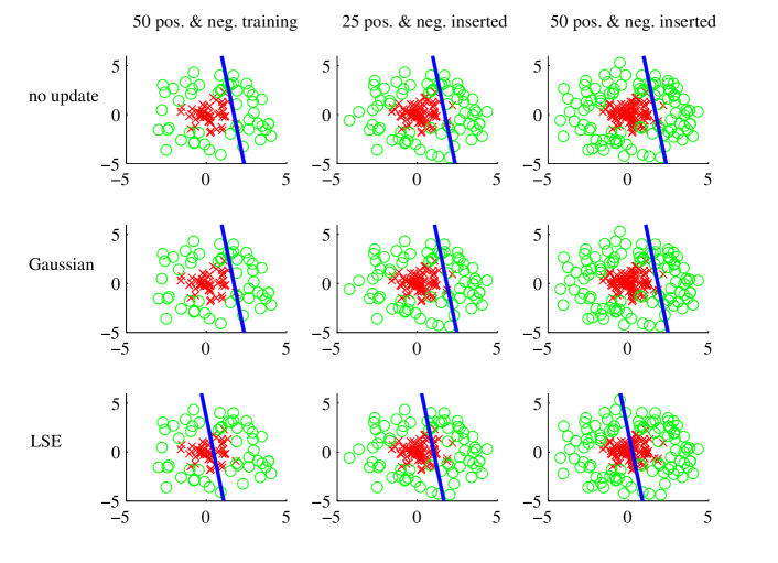
Figure 1: Toy data set. $\times$’s and $\circ$’s represent positive and negative samples, respectively. Top row: No update. The parameters of weak learners do not get updated. Middle row: Gaussian model. Linear classifier threshold is calculated from updated mean and variance (using (17)). Bottom row: Least square error. Linear classifier threshold is updated using linear regression. The leftmost column shows the classifier thresholds on the initial training set ($50$ positive and $50$ negative training points). The middle column shows the classifier thresholds with $25$ new positive and $25$ new negative points inserted. The rightmost column shows the thresholds with $50$ new positive and $50$ new negative inserted. Due to the asymmetry of the data distributions, updating the parameters of the weak learners could result in performance deterioration.

The online GSLDA framework is summarized in Algorithm LABEL:ALG:OGSLDA. Note that here we only use forward search of the original GSLDA algorithm of [24, 18]. In [19], we have shown that forward selection plus backward elimination improve the detection performance slightly but with extra computation.

Algorithm 2 The online GSLDA Algorithm.

7

7

7

7

7

II-C3 Incremental Learning Computational Complexity

Since, the initial training of online GSLDA is the same as offline GSLDA, we briefly explain the time complexity of GSLDA [19]. Let us assume we choose decision stumps as our weak learners. Let the number of training samples be $N$. Finding an optimal threshold of each feature needs $O(N\log{N}$). Assume that the size of the feature set is $M$. The time complexity for training weak learners is $O(MN\log{N})$. During GSLDA learning, we need to find mean $O(N)$, variance $O(N)$ and correlation $O(T^{2})$ for each feature. Since, we have $M$ features and the number of weak learners to be selected is $T$, the total time complexity for offline GSLDA is $O(MN\log{N}+MNT+MT^{3})$.

Given the selected set of weak learners, the time complexity of online GSLDA when new instance is inserted can be calculated as follows. Since, the number of weak learners is $T$, the total time complexity to calculate ${\boldsymbol{x}}$ in Step $1$ is $O(T)$. It also takes $O(T)$ to update the class mean in Step $2$. At Step $3$, calculating $U$, $V$, $r1$, $r2$ take $O(T^{2})$. In this step, the order in which we calculate the matrix-matrix multiplication affects the overall efficiency. Since, we are dealing with a small matrix chain multiplication, it is possible to go through each possible order and pick the most efficient one. For (14), we perform matrix-matrix multiplication in the following order $(((\Sigma_{0}^{-1}U)D^{-1})(V^{\!\top}\Sigma_{0}^{-1}))$. The number of operations required to compute $(\Sigma_{0}^{-1}U)$ is $O(T\times T\times 2)$, $((\Sigma_{0}^{-1}U)D^{-1})$ is $O(T\times 2\times 2)$, $(V^{\!\top}\Sigma_{0}^{-1})$ is $O(2\times T\times T)$ and $(((\Sigma_{0}^{-1}U)D^{-1})(V^{\!\top}\Sigma_{0}^{-1}))$ is $O(T\times 2\times T)$. Hence, the complexity of updating matrix inversion is still in the order of $O(T^{2})$. Since, the size of within-class matrix is $T\times T$, the matrix-vector multiplication in Step $4$ takes $O(T^{2})$. Updating classifier threshold in Step $5$ takes $O(T^{2})$ for the first criterion (First, we find the projected mean and covariance, $O(T)$ and $O(T^{2}+T)$, respectively. Then, we solve a closed-form second-degree polynomial). The second criterion in Step $5$ takes $O(T^{2})$ (Again, the time complexity of projected mean and covariance is $O(T)$ and $O(T^{2}+T)$). The third criterion in Step $5$ takes $O(T)$ (Here, we only have to calculate the dot product of two vectors). Hence, the time complexity of Step $5$ is at most $O(T^{2})$. Therefore, the total time complexity for online GSLDA with the insertion of a new instance is at most $O(\underbrace{N_{0}M\log N_{0}+N_{0}MT+MT^{3}}_{\text{Offline}}+\underbrace{T^{2}}_{\text{Online}})$. Here, $N_{0}$ is the number of initial training samples which assumed to be small. Note that the speed-up of online GSLDA over batch GSLDA is noticeable, i.e. $\underbrace{O(NT^{2})}_{\text{Online}}$ $\ll$ $\underbrace{O(N^{2}\log{N})}_{\text{Batch}}$, when more instances are inserted into the training set ($N\gg N_{0}$).

In terms of memory usage, between-class scatter matrix takes up $O(2T)$. The inverse of within-class scatter matrix occupies $O(T^{2})$. For the first and second criteria in Step $5$, we also need to keep the covariance matrices of $\Sigma_{1}$ and $\Sigma_{2}$ which takes up $O(2T^{2})$. Hence, the extra memory requirements for online GSLDA are at most $O(3T^{2}+2T)$. Given that the selected number of weak classifiers in each cascade layer is often small ($T<200$), the time and memory complexity of online GSLDA is almost negligible.

III Experiments

This section is organized as follows. The datasets used in this experiment, including how the performance is analyzed, are described. Experiments and the parameters used are then discussed. Finally, experimental results and analysis of different techniques are presented.

III-A USPS Digits Classification

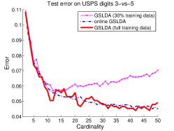
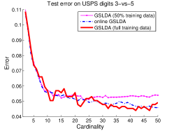
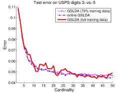
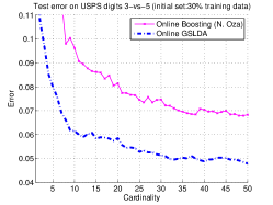
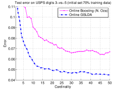
Figure 2: Top: Classification error rates by offline GSLDA and online GSLDA on $16\times 16$ pixels USPS digits data sets [29]. The number of initial training data for online GSLDA is (a) $30\%$, (b) $50\%$, (c) $70\%$ of the available training data. All experiments, except batch GSLDA (trained with full training sets), are run $10$ times. The mean of the errors are plotted. Bottom: Classification error rates by online GSLDA and online boosting [13]. The number of initial training data is (d) $30\%$, (e) $50\%$, (f) $70\%$ of the available training data. All experiments are run $10$ times.

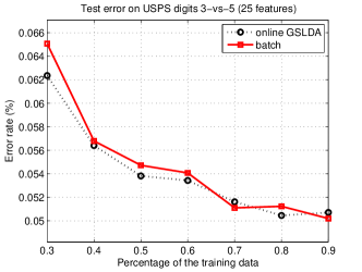
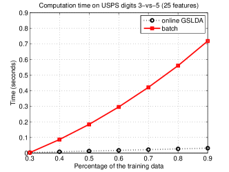
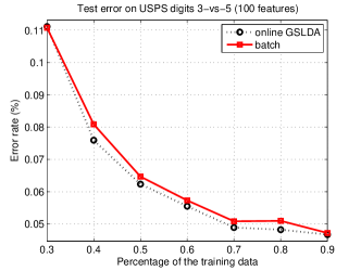
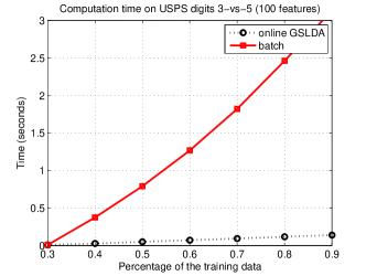
Figure 3: Comparison of classification error rate and computation cost between online GSLDA and batch GSLDA on $16\times 16$ pixels USPS digits data sets [29]. We set the number of nonzero components of the feature coefficients ($\ell_{0}$ norm) to $25$ (a,b) and $100$ (c,d).

We compare online GSLDA against batch GSLDA for classification of $16\times 16$ pixels USPS digits ‘$3$’ and ‘$5$’. The data set consists of $406$ training instances and $418$ test instances for the digit ‘$3$’, $361$ training instances and $355$ test instances for digit ‘$5$’ [29]. We use the raw intensity value as the features. Hence, the total number of features is $256$. For batch learning, we applied greedy approach to sequentially select feature which yields maximal class separation (forward search). We then evaluate the performance of the classifier on the given test set and measure the error rate [18]. For online learning, we randomly select $30/50/70$ percent training samples as the training set. Incremental updating is performed with the remaining training instances being inserted one at a time. We use decision stumps as the weak learners for both classifiers. All experiments, except batch GSLDA (trained with full training sets), are run $10$ times. The mean of the classification errors are plotted.

Figs. 2, 2 and 2 show the achieved classification error rates by batch GSLDA and online GSLDA. In the figures, the horizontal axis shows the $\ell_{0}$ norm of the feature coefficients, i.e., the number of weak classifiers, and the vertical axis indicates the classification error rate on test data. We observe a trend that the error rate decreases when we train with more training instances. It is important to point out that in this experiment the error rate of online GSLDA is quite close to that by batch GSLDA. We also train offline GSLDA classifiers with $30\%$, $50\%$ and $70\%$ training data. We observe an increase in error rates of GSLDA ($30\%$ training data) when the number of dimensions increase. This is not surprising since it is quite common for a classifier to overfit with large dimensions and small sample size.

We compare the performance of online GSLDA with online boosting proposed in [13]. For each weak classifier, we build a model by estimating the univariate normal distribution with weighted mean and variance for digits ‘$3$’ and ‘$5$’. We update the weak classifier by incrementally updating the mean and variance using weighted version of (II-C1) and (10). The results of online boosting are shown in Figs. 2, 2 and 2. The test error of online boosting decreases as the initial number of training samples increases. We observe that the performance of online boosting to be remarkably worse than the performance of online GSLDA.

Figs. 3 and 3 shows the achieved classification error rates by batch GSLDA and online GSLDA with $25$ and $100$ dimensions (features). In the figure, the horizontal axis shows the portion of training data instances and the vertical axis indicates the classification error rate. We observe a trend that the error rate decreases when more and more training data instances are involved, as expected. Online GSLDA not only performs well on this dataset but it is also very efficient. We give a comparison of the computation cost between batch GSLDA and incremental GSLDA in Figs. 3 and 3. As can be seen, the execution time of online GSLDA is significantly smaller than that of batch GSLDA as the number of training samples grows.

III-B Frontal Face Detection

Due to its efficiency, Haar-like rectangle features [8] have become a popular choice as image features in the context of face detection. Similar to the work in [8], the weak learning algorithm known as decision stumps and Haar-like rectangle features are used here due to their simplicity and efficiency. The following experiments compare offline GSLDA and online GSLDA learning algorithm.

III-B1 Performances on Single-node Classifiers

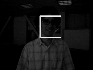
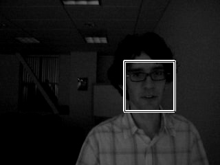
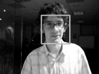
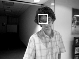
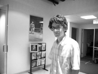
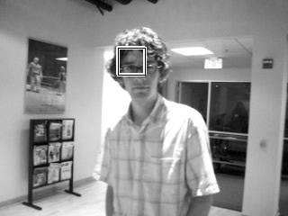
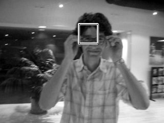
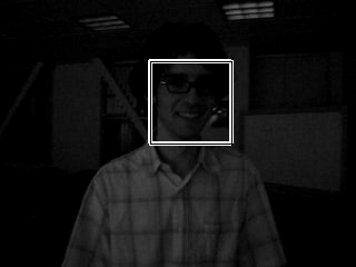
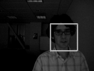
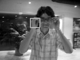
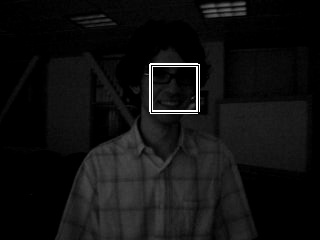
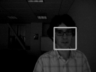
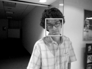
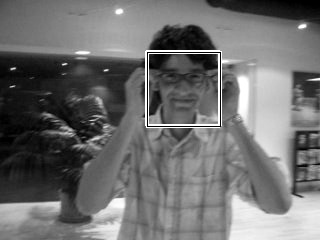
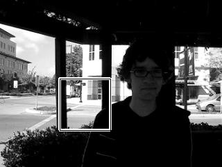
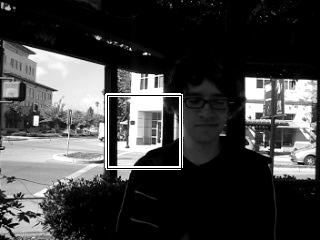
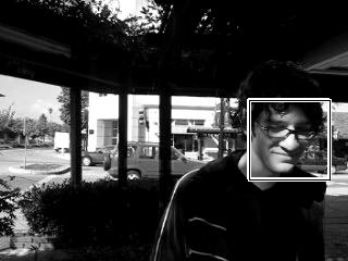
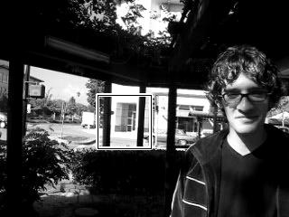
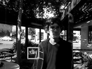
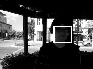
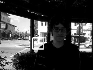
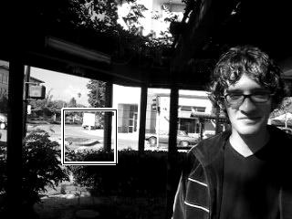
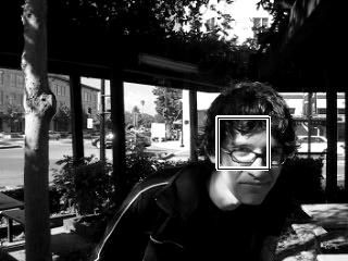
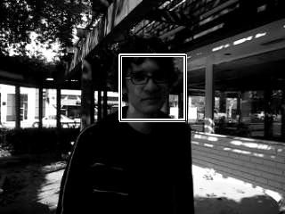
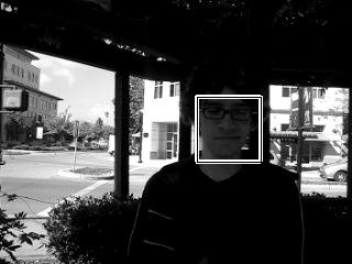
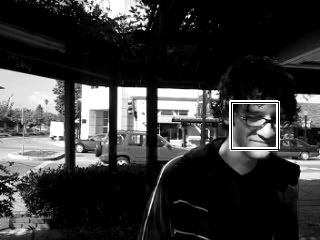
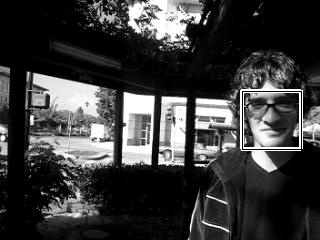
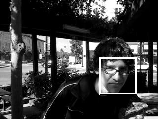
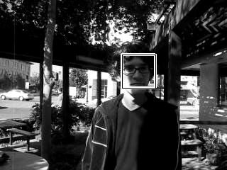
Figure 4: A comparison of offline AdaBoost based frontal face detector [8] (Top row), AsymBoost based face detector [28] (Second row), GSLDA based face detector [19] (Third row) and our proposed OGSLDA face detector (Last row). All detectors are trained initially with $1,000$ faces and $10,000$ non-faces. Online GSLDA is incrementally updated with patches classified as faces from the previous video frames. The first video (david indoor) contains $761$ frames of a person moving from a dark to a bright area undergoing large lighting and pose changes (frames $150$, $250$, $350$, $409$, $450$, $494$ and $592$). The second video (trellis) contains $501$ frames of a person moving underneath a trellis with large illumination change (frames $50$, $85$, $182$, $231$, $287$, $386$ and $457$).

We conduct two experiments in this section. The first experiment compares single strong classifier learned using AdaBoost [8], AsymBoost [28], offline GSLDA [19] and our proposed online GSLDA algorithms. The datasets consist of $1,000$ mirrored face examples (Fig. 6) and $10,000$ bootstrapped non-face examples. The face were cropped and rescaled to images of size $24\times 24$ pixels. For non-face examples, we initially select $1,000$ random non-face patches from non-face images. The other $9,000$ non-face patches are added to the initial pool of training data by bootstrapping.

We train three offline face detectors using AdaBoost, AsymBoost and GSLDA. Each classifier consists of 200 weak classifiers. The classifiers are tested on a challenged face videos, David Ross indoor data set and trellis data set, which are publicly available on the internet. Both videos contain large lighting variation, cast shadows, unknown camera motion, and tilted face with in-plane and out-of-plane rotation. The first video contains $761$ frames of a person moving from a dark to a bright area. Since, the first few video frames has very low contrast (almost impossible to see faces), we ignore the first $100$ frames. The second video contains $501$ frames of a person moving underneath a trellis with large illumination change and cast shadows.

In this experiment, we use the scanning window technique to locate faces. We set the scaling factor to $1.2$ and window shifting step to $1$. The patch with highest classification score is classified as faces. In other words, there is only one selected face in each frame. The criteria similar to the one used in PASCAL VOC Challenge [30] is adopted here. Detections are considered true or false positives based on the area of overlap with ground truth bounding boxes. To be considered a correct detection, the area of overlap between the predicted bounding box, $B_{p}$, and ground truth bounding box, $B_{gt}$, must exceed 50% by the formula:

$$\frac{area(B_{p}\cap B_{gt})}{area(B_{p}\cup B_{gt})}>50\%.$$

For online GSLDA, the predicted faces in the previous frames are used to update the GSLDA model. Note that the updated patches could contain both true positives (faces) and false positives (misclassified non-faces). After the update process, the classifier predicts a single patch with highest classification score in the next frame as the face patch. This learning technique is similar to semi-supervised learning where the classifier makes use of the unlabeled data in conjunction with a small amount of labeled data. Note that unlike the work in [14] where both positive and negative patches are used to incrementally update their model, we only make use of positive patches.

Table II compares the four face detectors in terms of their performance. We observe that the performance of AdaBoost face detector is the worst. This is not surprising since the distributions of training data are highly skewed ($1,000$ faces and $10,000$ non-faces). Viola and Jones also pointed out this limitation in [28]. Face detectors trained using AsymBoost and GSLDA perform quite similar on the first video. The results are consistent with the ones reported in [19]. Our results show that online GSLDA performs best. Based on our observations, incrementally updating GSLDA model improves the detection results significantly at small increase in computation time. Fig. 4 compares the empirical results between offline GSLDA and our proposed online GSLDA.

TABLE II: Performance on four different frontal face detectors on david indoor and trellis video

	detection rate
	indoor sequence	trellis sequence
AdaBoost [8]	$57.8\%$	$35.3\%$
AsymBoost [28]	$68.7\%$	$37.5\%$
GSLDA [19]	$70.3\%$	$48.5\%$
Our proposed OGSLDA	$83.1\%$	$62.1\%$

Finally, we compare the Receiver Operating Characteristic (ROC) curves between the offline GSLDA model ($1,000$ faces and $10,000$ non-faces) and the online GSLDA model (initially trained with $1,000$ faces and $10,000$ non-faces + updated with $661$ patches classified as faces). In this experiment, we set the scaling factor to $1.2$ and window stepping size to $1$. The techniques used for merging overlapping windows are similar to [8]. Detections are considered true or false positives based on the area overlap with ground truth bounding boxes. We shift the classifier threshold and plot the ROC curves (Fig. 5). Clearly, updating the trained model with relevant training data increases the overall performance of the classifiers.

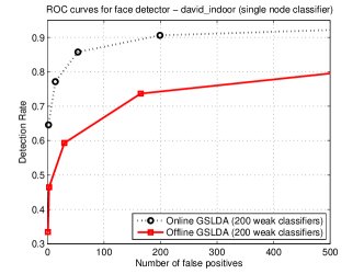
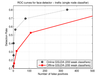
Figure 5: Comparison of ROC curves between offline and online GSLDA on David Ross indoor data set (top) and trellis data set (bottom).

Figure 6: A random sample of face images for training.

TABLE III: The size of training and test sets used on the single node classifier.

#	data splits	faces$/$split	non-faces$/$split
Train	$3$	$2000$	$2000$
Test	$2$	$2000$	$2000$

In the next experiment, we compare the performance of single strong classifiers learned using offline GSLDA and online GSLDA algorithms on frontal faces database. The database consists of $10,000$ mirrored faces. The faces were cropped and rescaled to images of size $24\times 24$ pixels. For non-face examples, we randomly selected 10,000 random non-face patches from non-face images obtained from the internet. The collected patches are split into three training sets and two test sets. Each set contains 2,000 face examples and 2,000 non-face examples (Table III). For each experiment, three different classifiers are generated, each by selecting two out of three training sets and the remaining training set for validation.

In this experiment, we train $30$, $50$ and $100$ weak learners of Haar-like features. The performance is measured by the test error rate. The results are shown in Fig. 7. The following observations can be made from these curves. The error of both classifiers drops as the number of training samples increases. The error rate of batch GSLDA drops at a slightly faster rate than online GSLDA. This is not surprising. For batch learning, the previous set of training samples along with a new sample are used to update the decision stumps every time a new sample is inserted. For each update, GSLDA algorithm throws away previously selected weak classifiers and reselects the new $30$, $50$ and $100$ weak classifiers. As a result, the training process is time consuming and requires a large amount of storage. In contrast, online GSLDA relies on the initial trained decision stumps. The new instance does not update the trained decision stumps but the between-class and within-class scatter matrices. The process is suboptimal compared to batch GSLDA. However, the slight increase in performance of batch GSLDA over online GSLDA ($0.7\%$ drop in test error rate for $100$ weak classifiers) comes at a much higher storage cost and significantly higher computation time.

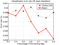
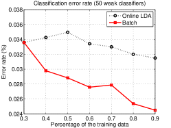
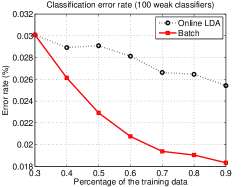
Figure 7: Comparison of classification error rates between batch GSLDA and online GSLDA. The number of weak learners (decision stumps on Haar-like features) in each experiment is (a) $30$, (b) $50$, (c) $100$. The error of both classifiers drops as the number of training samples increases.

III-B2 Performances on Cascades of Strong Classifiers

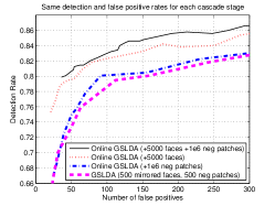
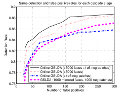
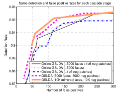
Figure 8: Comparison of ROC curves on MIT+CMU face test set. The four detectors are trained using (a) $500$ faces, (b) $1,000$ faces and (c) $5,000$ and $10,000$ mirrored faces.

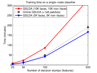
Figure 9: Comparison of the training time between GSLDA and online GSLDA algorithms. The first and second GSLDA detectors are trained with $5,000$ faces and $5,000$ non-faces, and $10,000$ faces and $10,000$ non-faces, respectively. Online GSLDA is initially trained with $5,000$ faces and $5,000$ non-faces and updated with one million new patches. Notice that there is a slight increase in training time even though we incrementally update with $200\times$ more training samples.

In this experiment, we use mirrored faces from previous experiment for batch learning and online learning. The number of initial positive samples used in each experiment is varied. We use $500$ faces, $1,000$ faces and $5,000$ faces to initially train a face detector. In each experiment, we trained four different cascaded detectors. The first cascaded detector is the same as in Viola and Jones [8] i.e., the face data set used in each cascade stage is the same while the non-face samples used in each cascade layer are collected from false positives of the previous stages of the cascade (bootstrapping). The cascade training algorithm terminates when there are not enough negative samples to bootstrap.

The second, third and forth face detectors are trained initially with the technique similar to the first cascaded detector. However, the second cascaded face detector is incrementally updated with new negative examples collected from false positives of the previous stages of cascade. The third cascaded face detector is incrementally updated with $5,000$ unseen faces. The final face detector is incrementally updated with both false positives from previous stages and unseen faces. For each face detector, weak classifiers are added to the cascade until the predefined objective is met. In this experiment, we set the minimum detection rate in each cascade stage to be $99\%$ and the maximum false positive rate to be $50\%$.

We tested our face detectors on the low resolution faces datasets, MIT+CMU frontal face test sets. The complete set contains $130$ images with $507$ frontal faces. In this experiment, we set the scaling factor to $1.2$ and window shifting step to $1$. The techniques used for merging overlapping windows is similar to [8]. Detections are considered true or false positives based on the area of overlap with ground truth bounding boxes. To be considered a correct detection, the area of overlap between the predicted bounding box and ground truth bounding box must exceed $50\%$. Multiple detections of the same face in an image are considered false detections.

Fig. 8 shows a comparison between the ROC curves produced by online GSLDA classifier. The ROC curves in Fig. 8 show that online GSLDA classifier outperforms GSLDA classifier at all false positive rates when initially trained with $500$ faces. Incrementally updating the GSLDA model with unseen faces ($+5000$ faces) yields a better result than updating the model with new false positives from previous stages of the cascade ($+10^{6}$ negative patches). The online classifier performs best when updated with both new positive and negative patches. Fig. 8 shows a comparison when the number of initial training samples have been increased to $1000$ faces. The performance gap between GSLDA and online GSLDA is now smaller. We observe the performance of both GSLDA and online GSLDA ($+10^{6}$ negative patches) to be very similar. This indicates that the cascade learning framework proposed by Viola and Jones might have already incorporated the benefit of massive negative patches. Incremental learning with new negative instances do not seem to improve the performance of cascaded detectors any further. Another way to explain the results of our findings is to use the concept of linear asymmetric classifier (LAC) proposed in [11]. In [11], the asymmetric node learning goal is expressed as

$$\mathop{\mathrm{maximize}}\limits_{{\boldsymbol{w}},w_{0}}\quad {\Pr}_{{\boldsymbol{x}}\sim({\boldsymbol{m}}_{1},\Sigma_{1})}\left\{{\boldsymbol{w}}^{\!\top}{\boldsymbol{x}}\geq w_{0}\right\},$$ (20)

$$\mathop{\mathrm{subject~{}to}}\nolimits\quad {\Pr}_{{\boldsymbol{y}}\sim({\boldsymbol{m}}_{2},\Sigma_{2})}\left\{{\boldsymbol{w}}^{\!\top}{\boldsymbol{y}}\leq w_{0}\right\}=\beta.$$

Since, the problem has no closed-form solution, the authors developed an approximate solution when $\beta=0.5$. To find a closed-form solution, the authors assumed that ${\boldsymbol{w}}^{\!\top}{\boldsymbol{x}}$ is Gaussian for any ${\boldsymbol{w}}$, class $C_{2}$ distribution is symmetric and the median value of the class $C_{2}$ distribution is close to its mean. The direction ${\boldsymbol{w}}$ can then be approximated by

$$\mathop{\mathrm{maximize}}\limits_{{\boldsymbol{w}}\neq 0}\quad\frac{{\boldsymbol{w}}^{\!\top}({\boldsymbol{m}}_{1}-{\boldsymbol{m}}_{2})}{\sqrt{{\boldsymbol{w}}^{\!\top}\Sigma_{1}{\boldsymbol{w}}}}.$$ (21)

From their objective functions, the only difference between FDA (5) and LAC (21) is that the pooled covariance matrix of FDA, $\Sigma_{1}$ + $\Sigma_{2}$, is replaced by the covariance matrix of class $C_{1}$, $\Sigma_{1}$. In other words, when train the classifier with the asymmetric node learning goal for the cascade learning framework, the variance of negative classes becomes less relevant. In contrast, new instances of positive classes affect both the numerator and denominator in (21). Hence, it is easier to notice the performance improvement when new positive instances are inserted. Our results seem to be consistent with their derivations.

We further increase the number of initial training faces to $5,000$. All face detectors now seem to perform very similar to each other. We conjecture that this is the best performance that our cascaded detectors with the provided training set can achieve on MIT+CMU data sets. The results of the face detectors trained with $10,000$ faces and $10,000$ non-faces seem to support our assumptions (Fig. 8). To further improve the performance, different cascade algorithms, e.g., soft-cascade [31], WaldBoost [32], multi-exit classifiers [33], etc. and a combination with other types of features, e.g., edge orientation histograms (EOH) [34], covariance features [35], etc., can also be experimented. Fig. 9 shows a comparison of the computation cost between batch GSLDA and online GSLDA. The horizontal axis shows the number of weak learners (decision stumps) and the vertical axis indicates the training time in minutes. From the figure, online learning is much faster than training a batch GSLDA classifier as the number of weak learners grows. On average, our online classifier takes less than $1.5$ millisecond to update a strong classifier of $200$ weak learners on standard off-the-shelf PC with the use of GNU scientific library (GSL).

IV Conclusion

In this work, we have proposed an efficient online object detection algorithm. Unlike many existing algorithms which applied boosting approach, our framework makes use of greedy sparse linear discriminant analysis (GSLDA) based feature selection which aims to maximize the class-separation criterion. Our experimental results show that our incremental algorithm does not only perform comparable to batch GSLDA algorithm but is also much more efficient. On USPS digits data sets, our online algorithm with decision stumps weak learners outperforms online boosting with class-conditional Gaussian distributions. Our extensive experiments on face detections reveal that it is always beneficial to incrementally train the detector with online samples. Ongoing works include the search for more accurate and efficient online weak learners.

Sakrapee Paisitkriangkrai is currently pursuing Ph.D. degree at the University of New South Wales, Sydney, Australia. He received the B.E. degree in computer engineering and M.E. degree in biomedical engineering from the University of New South Wales in 2003. His research interests include pattern recognition, image processing and machine learning.

Chunhua Shen received the Ph.D. degree from School of Computer Science, University of Adelaide, Australia, in 2005. Since Oct. 2005, he has been a researcher with the computer vision program, NICTA (National ICT Australia), Canberra Research Laboratory. He is also an adjunct research fellow at the Australian National University; and adjunct lecturer at the University of Adelaide. His main research interests include statistical machine learning and its applications in computer vision and image processing.

Jian Zhang (M’98-SM’04) received the Ph.D. degree in electrical engineering from the University College, University of New South Wales, Australian Defence Force Academy, Australia, in 1997. He is a principal researcher in NICTA, Sydney. He is also a conjoint associate professor at University of New South Wales. His research interests include image/video processing, video surveillance and multimedia content management. Dr. Zhang is currently an associate editor of the IEEE Transactions on Circuits and Systems for Video Technology and the EURASIP Journal on Image and Video Processing.

References

- [1] M-H. Yang, D. J. Kriegman, and N. Ahuja, “Detecting faces in images: A survey,” IEEE Trans. Pattern Anal. Mach. Intell., vol. 24, no. 1, pp. 34–58, 2002.
- [2] E. Hjelmas and B. K. Low, “Face detection: A survey,” Comp. Vis. Image Understanding, vol. 83, no. 3, pp. 236–274, 2001.
- [3] S. Munder and D. M. Gavrila, “An experimental study on pedestrian classification,” IEEE Trans. Pattern Anal. Mach. Intell., vol. 28, no. 11, pp. 1863–1868, 2006.
- [4] D. Gerónimo, A. M. López, A. D. Sappa, and T. Graf, “Survey on pedestrian detection for advanced driver assistance systems,” IEEE Trans. Pattern Anal. Mach. Intell., 21 May 2009. IEEE computer Society Digital Library. http://doi.ieeecomputersociety.org/10.1109/TPAMI.2009.122.
- [5] P. Campadelli, R. Lanzarotti, and G. Lipori, “Eye localization: a survey,” NATO Science Series, vol. 18, pp. 234–245, 2007.
- [6] Z. Sun, G. Bebis, and R. Miller, “On-road vehicle detection: a review,” IEEE Trans. Pattern Anal. Mach. Intell., vol. 28, no. 5, pp. 694–711, 2006.
- [7] C. Papageorgiou and T. Poggio, “A trainable system for object detection,” Int. J. Comp. Vis., vol. 38, no. 1, pp. 15–33, 2000.
- [8] P. Viola and M. J. Jones, “Robust real-time face detection,” Int. J. Comp. Vis., vol. 57, no. 2, pp. 137–154, 2004.
- [9] N. Dalal and B. Triggs, “Histograms of oriented gradients for human detection,” in Proc. IEEE Conf. Comp. Vis. Patt. Recogn., San Diego, CA, 2005, vol. 1, pp. 886–893.
- [10] M. T. Pham and T. J. Cham, “Fast training and selection of haar features using statistics in boosting-based face detection,” in Proc. IEEE Int. Conf. Comp. Vis., Rio de Janeiro, Brazil, 2007.
- [11] J. Wu, S. C. Brubaker, M. D. Mullin, and J. M. Rehg, “Fast asymmetric learning for cascade face detection,” IEEE Trans. Pattern Anal. Mach. Intell., vol. 30, no. 3, pp. 369–382, 2008.
- [12] R. Xiao, H. Zhu, H. Sun, and X. Tang, “Dynamic cascades for face detection,” in Proc. IEEE Int. Conf. Comp. Vis., Rio de Janeiro, 2007.
- [13] N. C. Oza and S. Russell, “Online bagging and boosting,” in Proc. Artificial Intell. & Statistics. 2001, pp. 105–112, Morgan Kaufmann.
- [14] H. Grabner and H. Bischof, “On-line boosting and vision,” in Proc. IEEE Conf. Comp. Vis. Patt. Recogn., Washington, DC, USA, 2006, pp. 260–267, IEEE Computer Society.
- [15] C. Huang, H. Ai, T. Yamashita, S. Lao, and M. Kawade, “Incremental learning of boosted face detector,” in Proc. IEEE Int. Conf. Comp. Vis., Rio de Janeiro, 2007, pp. 1–8.
- [16] T. Parag, F. Porikli, and A. Elgammal, “Boosting adaptive linear weak classifiers for online learning and tracking,” in Proc. IEEE Conf. Comp. Vis. Patt. Recogn., Anchorage, 2008, pp. 1–8.
- [17] X. Liu and T. Yu, “Gradient feature selection for online boosting,” in Proc. IEEE Int. Conf. Comp. Vis., Rio de Janeiro, 2007, pp. 1–8.
- [18] B. Moghaddam, Y. Weiss, and S. Avidan, “Fast pixel/part selection with sparse eigenvectors,” in Proc. IEEE Int. Conf. Comp. Vis., 2007, pp. 1–8.
- [19] S. Paisitkriangkrai, C. Shen, and J. Zhang, “Efficiently training a better visual detector with sparse eigenvectors,” in Proc. IEEE Conf. Comp. Vis. Patt. Recogn., Miami, Florida, June 2009.
- [20] S. Pang, S. Ozawa, and N. Kasabov, “Incremental linear discriminant analysis for classification of data streams,” IEEE Trans. Syst., Man, Cybern. B, vol. 35, no. 5, pp. 905–914, 2005.
- [21] J. Ye, Q. Li, H. Xiong, H. Park, R. Janardan, and V. Kumar, “IDR/QR: An incremental dimension reduction algorithm via QR decomposition,” IEEE Trans. Knowl. Data Eng., vol. 17, no. 9, pp. 1208–1222, 2005.
- [22] H. Zhao and P. C. Yuen, “Incremental linear discriminant analysis for face recognition,” IEEE Trans. Syst., Man, Cybern. B, vol. 38, no. 1, pp. 210–221, 2008.
- [23] R. Duda, P. Hart, and D. Stork, Pattern Classification (2nd ed.), John Wiley and Sons, 2001.
- [24] B. Moghaddam, Y. Weiss, and S. Avidan, “Generalized spectral bounds for sparse lda,” in Proc. Int. Conf. Mach. Learn., New York, NY, USA, 2006, pp. 641–648, ACM.
- [25] T.-K. Kim, S.-F. Wong, B. Stenger, J. Kittler, and R. Cipolla, “Incremental linear discriminant analysis using sufficient spanning set approximations,” in Proc. IEEE Conf. Comp. Vis. Patt. Recogn., Minneapolis, 2007, pp. 1–8.
- [26] R. Bru, J. M., J. Mas, and M. Tuma, “Balanced incomplete factorization,” SIAM J. Sci. Comput., vol. 30, pp. 2302–2318, 2008.
- [27] L. G. Rueda, “An efficient approach to compute the threshold for multi-dimensional linear classifiers,” Pattern Recogn., vol. 37, no. 4, pp. 811–826, 2004.
- [28] P. Viola and M. J. Jones, “Fast and robust classification using asymmetric adaboost and a detector cascade,” in Proc. Adv. Neural Inf. Process. Syst. 2002, pp. 1311–1318, MIT Press.
- [29] C. E. Rasmussen and C. K. I. Williams, Gaussian Processes for Machine Learning, MIT Press, 2006.
- [30] “The PASCAL visual object classes challenge (VOC 2007),” http://www.pascal-network.org/challenges/VOC/voc2007/index.html.
- [31] L. Bourdev and J. Brandt, “Robust object detection via soft cascade,” in Proc. IEEE Conf. Comp. Vis. Patt. Recogn., San Diego, CA, US, 2005, pp. 236–243.
- [32] J. Sochman and J. Matas, “Waldboost - learning for time constrained sequential detection,” in Proc. IEEE Conf. Comp. Vis. Patt. Recogn., 2005, vol. 2, pp. 150–156.
- [33] M. T. Pham, V. D. D. Hoang, and T. J. Cham, “Detection with multi-exit asymmetric boosting,” in Proc. IEEE Conf. Comp. Vis. Patt. Recogn., Alaska, US, 2008, pp. 1–8.
- [34] K. Levi and Y. Weiss, “Learning object detection from a small number of examples: The importance of good features,” in Proc. IEEE Conf. Comp. Vis. Patt. Recogn., Washington, DC, 2004, vol. 2, pp. 53–60.
- [35] C. Shen, S. Paisitkriangkrai, and J. Zhang, “Face detection from few training examples,” in Proc. IEEE Int. Conf. Image Process., 2008, pp. 2764–2767.