Theory of the Lightly Doped Mott insulator

Abstract

A theory for the Hubbard model appropriate in the limit of large $U/t$, small doping away from half-filling and short-ranged antiferromagnetic spin correlations is presented. Despite the absence of any broken symmetry the Fermi surface takes the form of elliptical hole pockets centered near $(\frac{\pi}{2},\frac{\pi}{2})$ with a volume proportional to the hole concentration. Short range antiferromagnetic correlations render the nearest neighbor hopping almost ineffective so that only second or third nearest neighbor hopping contributes appreciably to the dispersion relation.

I Introduction

The existence and shape of the Fermi surface and its change with doping may be one of the central issues in the physics of cuprate superconductors. Quantum oscillations consistent with Fermi liquid behaviour and a pocket-like Fermi surface have been observed in the underdoped compounds YBa₂Cu₃O_6.5Doiron ; Sebastian_1 ; Jaudet ; Audouard and YBa₂Cu₄O₈Yelland ; Bangura . Overdoped Tl₂Ba₂CuO_6+δ on the other hand shows quantum oscillations as well but a ’large’ Fermi surfaceVignolle consistent with band structure calculations. This indicates a change of the Fermi surface volume around optimal doping. Similarly, the electron doped compound Nd_2-xCe_xCuO₄ shows a pocket-like Fermi surface for electron concentrations up to $\delta=0.16$ and which changes abruptly to a large Fermi surface for $\delta=0.17$Helm . The transition in Nd_2-xCe_xCuO₄ thus occurs in an overdoped compound and therefore is unrelated to antiferromagnetic ordering.
The validity of a Fermi liquid description in underdoped cuprates is incompatible with the ’Fermi arc’ picture which is frequently invoked to describe the absence of a large Fermi surface in angle resolved photoemission spectroscopy (ARPES)dama . The Fermi surface of a Fermi liquid is a constant energy contour of the quasiparticle dispersion and thus necessarily a closed curve in ${\bf k}$-space. ARPES experiments on insulating antiferromagnets like Sr₂Cu₂O₂Cl₂Wells and Ca₂CuO₂Cl₂Ronning have shown that the valence band is consistent with next-nearest hopping - as in an antiferromagnet - with maximum close to $(\frac{\pi}{2},\frac{\pi}{2})$ and that the part of the quasiparticle band facing $(\pi,\pi)$ has very small spectral weight. Assuming that the effect of doping mainly consists in the chemical potential cutting into this quasiparticle band the Fermi surface would take the form of elliptical hole pockets and the ’Fermi arcs’ would simply be the portions of the pocket with large spectral weight. This has in fact been confirmed by the recent ARPES experiments on underdoped Bi₂(Sr_2-xLa_x)CuO₆ by Meng et al.Meng .
As for the quantum oscillation experiments the electron-like nature of the carriers suggested by the sign of both Hall constantLeBoeuf and thermopowerChang is incompatible with a straightforward interpretation in terms of hole pockets. Rather, the strong temperature dependence of the Hall constantRourke and the enhancement of low frequency magnetic excitations in a magnetic fieldHaug suggest a complicated and as yet not understood reconstruction process to take place in YBa₂Cu₃O_6.5 and YBa₂Cu₄O₈. Concerning the thermopower it has also been pointed out that in the cuprates there may be no obvious correspondence between the sign of the thermopower and the Fermi surface geometryTranquada .
In the present manuscript we investigate the point of view that hole pockets are a generic property of a lightly doped Mott insulator where the bulk of electrons continues to be localized as in the insulator and the mobile carriers correspond to the doped holes. The localized electrons retain only their spin degrees of freedom and do not contribute to the volume of the Fermi surface which leads to a Fermi surface with a volume proportional to the hole concentration irrespective of any broken symmetry. In fact, no experimental evidence for any staggered order parameter which would explain hole pockets by backfolding of a large Fermi surface has been found so far. Moreover this picture - a single mobile hole interacting with spin excitations - is the underlying one for all successful theories of the ARPES spectra of insulating compoundsaf2 ; af3 ; af4 ; af5 ; af6 ; af7 ; af8 ; af9 ; af10 .
Further motivation for the present work comes from exact diagonalization studies of the t-J model. These show that the Fermi surface at hole dopings $\leq 15\%$ takes the form of hole pocketspoc1 ; poc2 ; poc3 , that the quasiparticles have the character of strongly renormalized spin polarons throughout this doping ranger1 ; r2 ; r3 and that the low energy spectrum at these doping levels can be described as a Fermi liquid of spin $1/2$ quasiparticles corresponding to the doped holeslan . A comparison of the dynamical spin and density correlation function at low ($\delta<15\%$) and intermediate ($\delta=30-50\%$) hole doping moreover indicates that around optimal doping a phase transition takes place. In the underdoped regime spin and density correlation function differ strongly, with magnon-like spin excitations and extended incoherent continua in the density correlation functionden1 ; den which can be explained quantitatively by a calculation in the spin-polaron formalismbeckervoijta . At higher doping, spin and density correlation function become more and more similar and both approach the self-convolution of the single-particle Green’s function, whereby deviations from the self-convolution form can be explained as particle-hole excitations across a free electron-like (’large’) Fermi surfaceintermediate . This rough picture would be similar to the present experimental situation for cuprate superconductors.
Here we present a theory for the underdoped phase. We study the 2 dimensional (2D) Hubbard model

$$H = H_{t}+H_{U}$$

$$H_{t} = -\sum_{i,j}\sum_{\sigma}\;t_{ij}c_{i,\sigma}^{\dagger}c_{j,\sigma}$$

$$H_{U} = U\sum_{i}n_{i,\uparrow}n_{i,\downarrow}$$ (1)

where the nearest neighbor hopping $t_{10}=1$ and we fix $U/t_{10}=8$. The results depend only weakly on $U/t$ as long as this is sufficiently large. In addition we use $t_{11}=-0.1\;t_{10}$ and $t_{21}=-t_{11}/2$. These values of $t_{11}$ and $t_{20}$ are smaller than the generally accepted ones for cuprate superconductors - this will be discussed below.
In setting up a theory we have the following picture in mind: at half-filling - i.e. the Mott insulator - the electrons are localized and retain only their spin degrees of freedom. The hopping term creates charge fluctuations i.e. holes and double occupancies which we consider as spin-$\frac{1}{2}$ Fermions. The excitation spectrum of these Fermions has the well-known Hubbard gap of order $U$ which exsists irrespective of any kind of order or broken symmetry. In section II we set up the Hamiltonian for these charge fluctuations. Since we really want to study the doped system where apparently no broken symmetry exists we thereby consider a hypothetical insulating phase with no long range antiferromagnetic order but short ranged antiferromagnetic spin correlations i.e. the ’spin liquid’. The 2D Hubbard model has no broken symmetry at finite temperature so we believe it is quite reasonable to study the charge fluctuations in such a disordered phase. We then assume that for low doping $\delta$ this picture remains applicable, that means the holes created by doping have the same character as the holes created by charge fluctuations at half-filling. Whether this assumption is justified is a question to be answered by experiment, but we believe that the recent experimental results lend some support to this idea. Section III gives a summary and conclusions.

II Effective Hamiltonian for charge fluctuations

The basic idea of the calculation is the (approximate) diagonalization of the Hubbard Hamiltonian in a suitably chosen truncated Hilbert space. As a starting point for constructing the truncated Hilbert space we consider a state $|\Psi_{0}\rangle$ which has exactly one electron/site, is invariant under point group operations, has momentum zero and is a spin singlet. These are the quantum numbers of a vacuum state and indeed $|\Psi_{0}\rangle$ will play the role of a vacuum state, i.e. a state containing neither charge nor spin fluctuations. The only property of this state which will enter the calculation is the static spin correlation function

$$\chi_{ij}=\langle\Psi_{0}|{\bf S}_{i}\cdot{\bf S}_{j}|\Psi_{0}\rangle.$$ (2)

We consider $\chi_{ij}$ as given and do not attempt to compute it. We assume it to be antiferromagnetic and of short range i.e.

$$\chi_{ij}=C_{0}\;e^{i{\bf Q}\cdot({\bf R}_{i}-{\bf R}_{j})}e^{-\frac{|{\bf R}_{i}-{\bf R}_{j}|}{\zeta}}$$ (3)

where ${\bf Q}=(\pi,\pi)$. Moreover $\chi_{ij}$ has to obey the constraint

$$\sum_{j\neq 0}\chi_{0j}=-\frac{3}{4}$$ (4)

which follows from $|\Psi_{0}\rangle$ being a singlet. In practice we assume that (3) holds only for more distant than nearest neighbors and take the nearest neighbor spin correlation $\chi_{10}>-0.33$ in 2DRegerYoung as a first free parameter. Next we choose $\zeta$ and adjust $C_{0}$ for the longer range part of $\chi$ so as to fulfill (4). The results for the quasiparticle dispersion turn out to be almost independent of $\zeta$ and only weakly dependent on $\chi_{10}$.
Having specified the ’spin background’ $|\Psi_{0}\rangle$ we introduce the basis states of the truncated Hilbert space. Using the familiar Hubbard operators $\hat{d}_{i,\sigma}^{\dagger}=c_{i,\sigma}^{\dagger}n_{i,\bar{\sigma}}$ and $\hat{c}_{i,\sigma}^{\dagger}=c_{i,\sigma}^{\dagger}(1-n_{i,\bar{\sigma}})$ they take the form

$$2^{(N_{\nu}+N_{\mu})/2}\;\prod_{\nu=1}^{N_{\nu}}\hat{d}_{i_{\nu},\sigma_{\nu}}^{\dagger}\;\prod_{\mu=1}^{N_{\mu}}\hat{c}_{i_{\mu},\sigma_{\mu}}|\Psi_{0}\rangle.$$ (5)

These states have double occupancies and holes at specified positions and we treat these holes and double occupancies as weakly interacting spin-$\frac{1}{2}$ Fermions, which is the key approximation of the theory. Fermions are the only meanigful description for these particles because the Hubbard operators at different sites anticommute. Since $\langle\Psi_{0}|\hat{d}_{i,\sigma}\hat{d}_{i,\sigma}^{\dagger}|\Psi_{0}\rangle=\langle\Psi_{0}|\hat{c}_{i,\sigma}^{\dagger}\hat{c}_{i,\sigma}|\Psi_{0}\rangle=\frac{1}{2}$ the states (5) are approximately normalized if the average distance between the holes and double occupancies is larger than the spin correlation length $\zeta$ (see below). This condition is satisfied in the limit of large $U$, small doping and short spin correlation length, which is the case of interest.
A key problem in setting up a theory for the charge fluctuations in the Hubbard model is the peculiar nature of holes and double occupancies. Both a hole and double occupany are spinless objects. Despite this, for example the states $\hat{d}_{i,\uparrow}^{\dagger}|\Psi_{0}\rangle$ and $\hat{d}_{i,\downarrow}^{\dagger}|\Psi_{0}\rangle$ are orthogonal. In fact, acting with $\hat{d}_{i,\sigma}^{\dagger}$ implies a projection onto the component of $|\Psi_{0}\rangle$ which has a $\bar{\sigma}$ electron on site $i$. While the newly created double occupancy is a spinless object, the information about the spin of the added electron therefore is ’stored’ in the ’spin background’ and it is in a sense stored within a spatial region of extend $\zeta$ around the respective double occupany/hole. This can be seen by considering expressions like

$$\langle\Psi_{0}|\hat{c}_{i,\uparrow}^{\dagger}\hat{d}_{j,\uparrow}\hat{d}_{j,\uparrow}^{\dagger}\hat{c}_{i,\uparrow}|\Psi_{0}\rangle = \frac{1}{4}-\frac{1}{3}\chi_{ij}$$

$$\langle\Psi_{0}|\hat{c}_{i,\downarrow}^{\dagger}\hat{d}_{j,\uparrow}\hat{d}_{j,\uparrow}^{\dagger}\hat{c}_{i,\downarrow}|\Psi_{0}\rangle = \frac{1}{4}+\frac{1}{3}\chi_{ij}$$

$$\langle\Psi_{0}|\hat{c}_{i,\uparrow}^{\dagger}\hat{d}_{j,\downarrow}\hat{d}_{j,\uparrow}^{\dagger}\hat{c}_{i,\downarrow}|\Psi_{0}\rangle = -\frac{2}{3}\chi_{ij}$$

$$\langle\Psi_{0}|\hat{c}_{i,\downarrow}^{\dagger}\hat{d}_{j,\downarrow}\hat{d}_{j,\uparrow}^{\dagger}\hat{c}_{i,\uparrow}|\Psi_{0}\rangle = -\frac{2}{3}\chi_{ij}$$ (6)

and similar ones. If the spin correlation function $\chi$ were zero in these and similar expressions the states (5) would indeed be normalized. In the following we neglect the corrections due to a finite $\chi$ in overlap matrix elements such as (6). This is probably the most problematic approximation in the present theory and induces some inaccuracies - as will be discussed below. Once we neglect the overlap at short distances, however, the states (5) are indeed normalized.
Finally, the holes and double occupancies have to obey a hard-core constraint i.e. there may be at most one particle per site. In the case of small $\delta$/large $U/t$, however, the density of these particles is small so that it is probably a good approximation to neglect the hard core constraint, see Appendix A for a comparison of the present theory with linear spin wave theory where the hard core constraint between magnons is neglected as well.
The procedure to be applied then is quite simple: the states (5) are represented by states of fictitious Fermionic spin-$\frac{1}{2}$ quasiparticles

$$\prod_{\nu=1}^{N_{\nu}}d_{i_{\nu},\sigma_{\nu}}^{\dagger}\;\prod_{\mu=1}^{N_{\mu}}h_{i_{\mu},\bar{\sigma}_{\mu}}^{\dagger}|0\rangle.$$ (7)

This means we have hole-like quasiparticles $h_{i_{\nu},\sigma_{\nu}}^{\dagger}$ and the double occupancy-like quasiparticles $d_{i_{\nu},\sigma_{\nu}}^{\dagger}$. All operators in the quasiparticle Hilbert space are defined by demanding that they their matrix elements between the states (7) are identical to those of the physical operators between the corresponding states (5).
We now use this procedure to set up the quasiparticle Hamiltonian. One has

$$\langle\Psi_{0}|\hat{c}_{j,\sigma}^{\dagger}\hat{d}_{i,\sigma}\;H_{t}\;|\Psi_{0}\rangle = -t_{ij}(\frac{1}{4}-\chi_{ij})$$

$$\langle\Psi_{0}|\hat{d}_{i,\sigma}\;H_{t}\;\hat{d}_{j,\sigma}^{\dagger}|\Psi_{0}\rangle = -t_{ij}(\frac{1}{4}+\chi_{ij})$$

$$\langle\Psi_{0}|\hat{c}_{j,\sigma}^{\dagger}\;H_{t}\;\hat{c}_{i,\sigma}|\Psi_{0}\rangle = \;\;\;t_{ij}(\frac{1}{4}+\chi_{ij})$$ (8)

These matrix elements describe the pair creation of a hole/double occupancy, the propagation of a double occupancy and the propagation of a hole. Thereby modifications due to nearby additional particles are neglected but again this will be reasonable for small particle density and short spin correlation length. Denoting

$$V_{ij} = -t_{ij}(\frac{1}{2}-2\chi_{ij})$$

$$\tilde{t}_{ij} = \;\;t_{ij}(\frac{1}{2}+2\chi_{ij})$$ (9)

the Hamiltonian governing the quasiparticles therefore is

$$H = -\sum_{ij,\sigma}\tilde{t}_{ij}\left(d_{i,\sigma}^{\dagger}d_{j,\sigma}-h_{i,\sigma}^{\dagger}h_{j,\sigma}\right)$$ (10)

$$\;\;\;+\sum_{ij,\sigma}V_{ij}\left(d_{i,\sigma}^{\dagger}h_{j\bar{\sigma}}^{\dagger}+h_{j\bar{\sigma}}d_{i,\sigma}\right)$$

$$\;\;\;\;\;\;+U\;\sum_{i,\sigma}d_{i,\sigma}^{\dagger}d_{i,\sigma}$$

The last term takes into account the fact that each double occupancy increases the energy by $U$.The extra factor of $2$ in (9) as compared to (8) takes into account the factor of $2^{(N_{\nu}+N_{\mu})/2}$ in (5).
The Hamiltonian (10) is solved by the transformation

$$\gamma_{{\bf k},+,\sigma}^{\dagger} = \;\;u_{{\bf k}}\;d_{{\bf k},\sigma}^{\dagger}+v_{{\bf k}}\;h_{-{\bf k}\bar{\sigma}}$$

$$\gamma_{{\bf k},-,\sigma}^{\dagger} = -v_{{\bf k}}\;d_{{\bf k},\sigma}^{\dagger}+u_{{\bf k}}\;h_{-{\bf k}\bar{\sigma}}$$ (11)

and we obtain the energies

$$E_{\pm}({\bf k}) = \tilde{\epsilon}_{\bf k}+\frac{U}{2}\pm W_{\bf k}$$

$$W_{\bf k} = \sqrt{(\frac{U}{2})^{2}+V_{\bf k}^{2}}$$ (12)

and the coefficients

$$u_{{\bf k}} = \sqrt{\frac{W_{{\bf k}}+\frac{U}{2}}{2W_{{\bf k}}}}$$

$$v_{{\bf k}} = \sqrt{\frac{W_{{\bf k}}-\frac{U}{2}}{2W_{{\bf k}}}}\;sign(V_{\bf k})$$ (13)

Since $c_{{\bf k},\sigma}=\hat{d}_{{\bf k},\sigma}+\hat{c}_{{\bf k},\sigma}$ the representation of the electron annihilation operator in the quasiparticle Hilbert space becomes

$$c_{{\bf k},\sigma}\rightarrow\frac{1}{\sqrt{2}}(d_{{\bf k},\sigma}+h_{-{\bf k},\bar{\sigma}}^{\dagger})$$ (14)

where the factor of $1/\sqrt{2}$ again is due to the prefactor in (5). The spectral weight of the two bands therefore is

$$Z_{\pm}({\bf k}) = \frac{1}{2}(u_{{\bf k}}\pm v_{{\bf k}})^{2}$$ (15)

$$= \frac{1}{2}\left(1\pm\frac{V_{{\bf k}}}{W_{{\bf k}}}\right)$$

If we set $\chi_{ij}=0$ both $\tilde{\epsilon}_{\bf k}$ and $-V_{\bf k}$ reduce to $\epsilon_{\bf k}/2$, with $\epsilon_{\bf k}$ the noninteracting band energy and we obtain

$$E_{\pm}({\bf k}) = \frac{1}{2}\left(\epsilon_{\bf k}+U\pm\sqrt{\epsilon_{\bf k}^{2}+U^{2}}\right),$$

$$Z_{\pm}({\bf k}) = \frac{1}{2}\left(1\mp\frac{\epsilon_{\bf k}}{\sqrt{\epsilon_{\bf k}^{2}+U^{2}}}\right),$$ (16)

which is identical to the result of the Hubbard-I approximationHubbard at half-filling. The present theory thus may be viewed as an extension of the Hubbard-I approximation to take into account the effect of finite spin correlations. The spin correlations, however, do have a drastic effect: for $\chi_{10}=-0.25$ the nearest neighbor hopping matrix element $\tilde{t}_{10}$ is zero. Here one has to bear in mind that the value of $\chi_{10}$ in the ground state of the Heisenberg antiferromagnet on the 2D square lattice with nn exchange only is $\approx-0.33$RegerYoung - a slight reduction of the spin correlations due to hole doping and longer range exchange may well produce a value very close to $-0.25$. For small $\tilde{t}_{10}$, however, the quasiparticle dispersion is dominated by next-nearest neighbor hopping and the quasiparticle dispersion is ’almost antiferromagnetic’ and thus quite different from the Hubbard-I approximation.
The second major difference between the present theory and the Hubbard-I and similar approximations is the way in which electrons are counted. In the quasiparticle Hilbert space the operator of electron number obviously is

$$N_{e}=N+\sum_{i,\sigma}(d_{i,\sigma}^{\dagger}d_{i,\sigma}-h_{i,\sigma}^{\dagger}h_{i,\sigma})$$ (17)

because the ’spin background’ $|\Psi_{0}\rangle$ contributes $N$ electrons (with $N$ the number of sites), each double occupancy increases the number of electrons by one and each hole decreases the number of electrons by one. When applied to a quasiparticle state of the type (7) the operator (17) therefore gives the same electron number as the physical electron operator applied to the corresponding Hubbard model state (5) and this is the prescription how operators in the quasiparticle Hilbert space are to be constructed. After transformation to the $\gamma$’s and treating these as noninteracting Fermions we obtain

$$N_{e}=\sum_{{\bf k},\sigma}\;(\;\gamma_{{\bf k},+,\sigma}^{\dagger}\gamma_{{\bf k},+,\sigma}+\gamma_{{\bf k},-,\sigma}^{\dagger}\gamma_{{\bf k},-,\sigma}\;)-N.$$ (18)

At half-filling, $N_{e}=N$, the lower of the two bands is completely filled, the upper one completely empty, which agrees with the Hubbard-I approximation. As the systems is doped away from half-filling, however, the Fermi surface volume has a volume which is strictly proportional to the number of doped holes - i.e. one has hole pockets with a total volume of $\delta/2$. These do not occur as a consequence of backfolding the Brillouin zone due to any kind of broken symmetry.
Pockets with a volume of $\delta/2$ are different from the Hubbard-I approximation and the reason is that there one uses a different way to count electrons, namely the integrated photoemission weight. Treating the $d$ and $h$ as ordinary Fermion operators, and using (14) we obtain the integrated spectral weight as

$$\tilde{N}_{e} = N+\frac{1}{2}\sum_{{\bf k},\sigma}\langle\;d_{{\bf k},\sigma}^{\dagger}d_{{\bf k},\sigma}-h_{{\bf k},\sigma}^{\dagger}h_{{\bf k},\sigma}\;\rangle$$ (19)

$$\;\;\;+\frac{1}{2}\sum_{{\bf k},\sigma}\langle\;d_{{\bf k},\sigma}^{\dagger}h_{{-\bf k}\bar{\sigma}}^{\dagger}+h_{-{\bf k}\bar{\sigma}}d_{{\bf k},\sigma}.\;\rangle$$

which differs from (17). There are several reasons for this discrepancy: first of all we have

$$\sum_{{\bf k}}\langle\;d_{{\bf k},\sigma}^{\dagger}h_{{-\bf k}\bar{\sigma}}^{\dagger}\;\rangle=\sum_{i}\langle\;d_{i,\sigma}^{\dagger}h_{i\bar{\sigma}}^{\dagger}\;\rangle$$ (20)

The latter expectation value, however, should be zero, because a hole and a double occupancy cannot occupy the same site. Even with this term omitted, however, there is an extra factor of $1/2$ and reason is a more fundamental one, namely the restriction of the Hilbert space. In fact it is easy to see that the spectral weight sum-rule cannot be applied to an approximation like the present one where the spectral weight is artificially concentrated in a single band. Let us consider a Fermi liquid with quasiparticle weight $Z<1$ and assume that one electron is removed at the Fermi energy. This implies that one momentum/spin crosses from the occupied to the unoccupied side of the Fermi energy which decreases the integrated photoemission weight by $Z$. The remaining weight of $1-Z$ therefore must disappear from the high-energy part of the photoemission spectrum and reappear in the high-energy part of the inverse photoemission spectrum. This is in fact exactly what is seen in exact diagonalization studies of the t-J model: there on has a quasiparticle band of width $\approx 2J$ and quasiparticle weight $Z\approx 0.1-0.5$ while most of the spectral weight resides in extended incoherent continuaszc ; dago1 . Upon doping the quasiparticle peak at the top of the band crosses the chemical potential while simultaneously spectral weight is removed from the incoherent part of the spectrum at energies of order $t$ below the Fermi energy. This weight reappears - in the form of multi-magnon excitations - at energies of order $J$ above the chemical potential and near $(\pi,\pi)$r1 (another way is realized in SDW mean-field theory for the Hubbard model, where the weight $Z$ crosses at ${\bf k}$ and the remaining weight $1-Z$ at ${\bf k}+{\bf Q}$). In a theory like the present one where all spectral weight is concentrated in one quasiparticle band, however, these high-energy parts do not exist and it is therefore impossible to maintain the spectral weight sum rule. In fact, for each electron removed from the system, $Z^{-1}$ momenta would have to cross from photoemission to inverse photoemission to maintain the sum-rule and it therefore is misleading to use the integrated photoemisssion weight to determine the Fermi surface volume. We have to accept that the spectral weight sum rule will not be fulfilled as a consequence of the restriction of the Hilbert space and the lack of the incoherent part of the spectra (this may be remedied at least partially by including the coupling to spin excitations so as to reproduce the incoherent continua). Instead, the correct expression for the particle number is given by (17).
In many calculations where the Hubbard-I approximation - or any other approximation involving Hubbard operators - is applied to the doped case, the analogue of (19) is used to calculate the electron number. This leads to the peculiar ’fractional’ dependence of the Fermi surface volume on hole doping because of the fractional number $Z^{-1}$ of momenta needed to fulfill the spectral weight sum-rule.
We proceed with a qualitative discussion of the band dispersion. Since we expect the theory to be valid only for $t\ll U$ we thereby expand in terms of $t/U$ and keep only the lowest nonvanishing order. Moreover we note that there are two additional small parameters. For the nearest neighbor spin correlation function $\chi_{10}$ close to $-\frac{1}{4}$, the effective nearest neighbor hopping $\tilde{t_{10}}$ is small. The value of $\chi_{10}$ in the GS of the 2D Heisenberg antiferromagnet with nearest-neighbor exchange is $-0.33$RegerYoung , so that a slight reduction due to doping/longer range hopping may well produce a value which is very close to $-\frac{1}{4}$. Moreover, in the CuO₂ plane the $(1,1)$ and $(2,0)$ hopping integrals fulfill $t_{11}/t_{20}\approx-2$. This equation holds if the underlying mechanism for these matrix elements is hopping of a Zhang-Rice singlet via Cu 4s orbitals. If the spin correlations $\chi_{11}$ and $\chi_{20}$ do not differ strongly we expect both $\tilde{t}_{11}+2\tilde{t}_{20}=\tau$ and $\tilde{V}_{11}+2\tilde{V}_{20}=\tilde{\tau}$ to be small.
Expanding to lowest order in $t/U$ we have

$$E_{-}({\bf k}) = \tilde{\epsilon}_{\bf k}-\frac{V_{\bf k}^{2}}{U}$$ (21)

and if $\tilde{t}_{10}$ is sufficiently small we expect the maximum of the lower band to be near $(\frac{\pi}{2},\frac{\pi}{2})$. At half filling the GS energy is

$$E_{0} = 2\sum_{\bf k}(E_{-}({\bf k})-\tilde{\epsilon}_{\bf k})$$ (22)

$$= -2zN\sum_{\alpha}\;J_{\alpha}\left(\chi_{\alpha}-\frac{1}{4}\right)^{2}$$

Here $\alpha\in\{10,11,20\dots\}$ labels the different shells of neighbors of a given site and $J_{\alpha}=4t_{\alpha}^{2}/U$. The true expectation value of the Heisenberg antiferromagnet in the state $|\Psi_{0}\rangle$ would be obtained by replacing $-4\left(\chi_{\alpha}-\frac{1}{4}\right)^{2}\rightarrow\chi_{\alpha}-\frac{1}{4}$. For nearest neighbor hopping only and $\chi_{1}\approx-0.33$ the above result therefore is a factor of $2.3$ too large. The discrepancy is due to the neglect of overlap integrals such as (6), see Appendix B. The inclusion of such overlap integrals probably is only a technical problem but we have to bear in mind that the simplification of neglecting such overlap integrals results in inaccuracies.
Next we consider the quasiparticle dispersion relation. As already mentioned if $\tilde{t}_{10}$ is small we expect the maximum of the dispersion of the lower band near $(\frac{\pi}{2},\frac{\pi}{2})$. Setting $k_{\alpha}=\frac{\pi}{2}+\kappa_{\alpha}$ and expanding to second order in $\kappa$ the constant energy contours are elliptical

$$E_{-}({\bf\kappa})=E_{max}-\frac{(\kappa_{+}-\kappa_{0})^{2}}{a^{2}}-\frac{\kappa_{-}^{2}}{b^{2}}$$ (23)

with $\kappa_{\pm}=\frac{1}{\sqrt{2}}(\kappa_{x}\pm\kappa_{y})$ and - neglecting terms $\propto\tau,\tilde{\tau}$ as well as terms of higher order in $t/U$ - one finds

$$\frac{1}{a^{2}} = \;\;2J_{10}\;(\frac{1}{2}-2\chi_{10})^{2}$$

$$\frac{1}{b^{2}} = -4t_{11}(\frac{1}{2}+2\chi_{11})$$

$$\frac{\kappa_{0}}{a^{2}} = \sqrt{2}\left(t_{10}\;(\frac{1}{2}+2\chi_{10})+J_{10}\frac{t_{11}}{t_{10}}(\frac{1}{2}-2\chi_{10})(\frac{1}{2}-2\chi_{11})\right)$$

Depending on the sign of $\chi_{10}+\frac{1}{4}$ the pockets thus are shifted towards $\Gamma$ or away from $\Gamma$.
It turns out that the correlation length $\zeta$ has negligible influence on the dispersion. More significant is the value of the nearest neighbor spin correlation function $\chi_{10}$. Figure 1 shows the quasiparticle dispersion and the spectral weight of the band for two values of $\chi_{10}$.

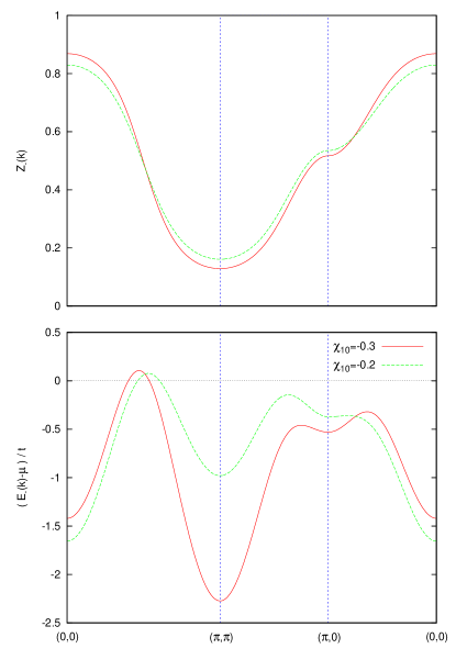
Figure 1: (Color online) Lower panel: dispersion of the lower band at $\delta=0.1$ for different values of $\chi_{10}$. Upper panel: dispersion of the spectral weight of the quasiparticle band. The correlation length $\zeta=4$.

Figure 2 shows the pockets obtained for the two different values of $chi_{10}$, which obviously determines the position of the hole pocket in the Brillouin zone. The pockets are not centered at $(\frac{\pi}{2},\frac{\pi}{2})$, for the larger values of $\chi_{10}$ the pocket is shifted towards $(0,0)$ as it is seen in the ARPES experimentMeng . The overall shape of the dispersion relation is quite similar as the one for a hole in an antiferromagnetBula ; Trugman ; Shraiman ; Inoue ; Ederbecker but it should be noted that the present theory does not use any antiferromagnetic order. The ’antiferromagnetic shape’ of the dispersion is due to the fact that even short range antiferromagnetic correlations combined with the strong Coulomb repulsion between electrons are sufficient to suppress the nearest neighbor hopping almost completely. More detailed calculations show that antiferromagnetic spin correlations instead enhance the incoherent nearest neighbor hopping, i.e. nearest neighbor hopping involves emisssion or absorption of a spin excitationtobepub . It also should be noted that the spectral weight of the ’backside’ of the pocket, i.e. the part facing $(\pi,\pi)$ is low. This is also seen in ARPESWells ; Ronning ; Meng , although the difference of spectral weight is much more pronounced there. By analogy with hole motion in an antiferromagnet one may assume, however, that the coupling to spin excitation and formation of spin polarons will enhance the difference in spectral weight and thus make the theory more similar to experimentwrobel .

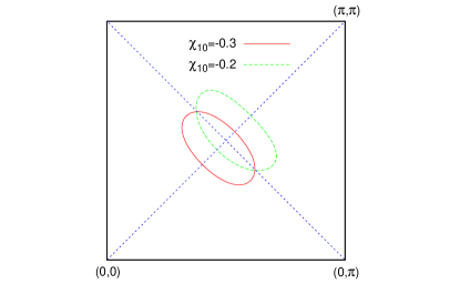
Figure 2: (Color online) Fermi surface at $\delta=0.1$ for different values of $\chi_{10}$. The correlation length $\zeta=4$.

It should be noted that the antiferromagnetic correlations determine the location of the pocket in the Brillouin zone but not the volume of the Fermi surface, which is given by (18). As already mentioned, if one sets the spin correlation function $\chi=0$ - which actually violates the singlet condition (4) - the dispersion relation agrees with that of the Hubbard I approximation and the hole pocket is then centered at $(\pi,\pi)$. A hole pocket around $(\pi,\pi)$ has indeed been observed in Quantum Monte Carlo (QMC) simulations of the Hubbard modelCarsten and it is plausible that the high temperature used in the (QMC) simulation renders the spin correlation function small or zero and thus shifts the pockets to the corner of the Brillouin zone.
Finally we note that the present theory tends to overestimate the impact of the $t_{11}$- and $t_{20}$-terms on the quasiparticle dispersion which is why we used relatively small values of $t_{11}$ and $t_{20}$ used here. This is probably related the fact that no coupling to spin excitations is taken into account in the present theory which increases the quasiparticle weight and the effect of the $t_{11}$- and $t_{20}$-terms.
To conclude this section we return to the issue of the hard-core constraint between the holes/double occupancies. To that end we consider the total densities of holes/double occupancies per spin direction:

$$n_{d} = \frac{1}{N}\;\sum_{i}\langle\;d_{i,\sigma}^{\dagger}d_{i,\sigma}\;\rangle$$

$$= \frac{1}{N}\;\sum_{\bf k}v_{\bf k}^{2}\;f(E_{-}({\bf k}))$$

$$n_{h} = \frac{1}{N}\;\sum_{i}\langle\;h_{i,\sigma}^{\dagger}h_{i,\sigma}\;\rangle$$

$$= \frac{1}{N}\;\sum_{\bf k}\left(v_{\bf k}^{2}+u_{\bf k}^{2}(1-f(E_{-}({\bf k})))\right)$$

This may serve as a criterion for the quality of the approximation to relax the hard-core constraint. Namely the probability for violation of the constraint at a given site is

$$p_{v}=4n_{d}n_{h}+n_{d}^{2}+n_{h}^{2}$$ (26)

and this is shown in Figure 3 for $U/t=8$ as a function of the hole concentration $\delta$. This implies that even at $\delta=0.2$ the constraint is violated at $5\%$ of the sites. Enforcement of the constraint e.g. by Gutzwiller projection would therefore have a small influence on the results. The neglect of the constraint therefore is probably a quite reasonable approximation.

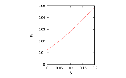
Figure 3: (Color online) Probability $p_{v}$ for violation of the hard-core constraint as a function of the hole concentration $\delta$. The finite value of $p_{v}$ at $\delta=0$ is due to the charge fluctuations at half-filling.

III Summary and Discussion

In summary a theory for the lightly doped Mott insulator has been derived. The basic assumption thereby is that holes introduced by doping have the same nature as the hole-like charge fluctuations at half-filling whose density is $\propto(\frac{t^{2}}{U^{2}})$. For low hole doping this is probably a reasonable assumption. The quasiholes then form a Fermi gas with a total Fermi surface volume of $\delta/2$. Antiferromagnetic spin correlations render the nearest neighbor hopping essentially ineffective so that the dispersion relation is similar to the one for hole motion in an antiferromagnet even in the complete absence of static antiferromagnetic order. The Fermi surface thus takes the form of four elliptical hole pockets centered near $(\frac{\pi}{2},\frac{\pi}{2})$. In addition to these Fermionic excitations the doped insulator probably has a second type of excitations, namely Bosonic spin triplet excitations which are similar in character as the magnons at half-filling. We postpone the discussion of these excitations and their interaction with the charge fluctuationstobepub .
A number of simplifying assumptions of different quality were made: the spin correlation function of the ’spin background’ was assumed to have a simple form and was taken as a given input parameter. It would be desirable to calculate this e.g. be minimization of the total energy but this would require a solution of the system of interacting quasiparticles and magnons. On the other hand the form of the spin correlation function which was assumed seems quite physical and moreover the results do not change strongly with the parameters of the spin correlation funtion. For example the quasiparticle dispersion is essentially independent of the spin correlation legth $\zeta$.
In solving the Hamiltonian for the charge fluctuations the overlap between pairs of particles has been neglected. This is probably the most drastic approximation made and was shown to lead to inaccuracies in the results e.g. a deviation from the ground state energy at half-filling from the known energy of the Heisenberg antiferromagnet. The neglected overlaps - being ’four particle overlaps’ - would create an interaction between the quasiparticles. The neglect of the hard-core constraint between the particles, on the other hand, is probably a very reasonable approximation because the density of the charge fluctuations is small.
An interesting question and possibly the key to understand high-temperature superconductivity is the nature of the phase transition between this correlation-dominated low doping phase with a hole-pocket-like Fermi surface and the intermediate and electron-density phase with a ’large’ Fermi surface which has been inferred e.g. from the dynamical spin and density correlation functionintermediate . Experimental data suggest that this phase transition occurs at optimal doping or in the overdoped range of hole concentrations and thus is related to the mechanism of superconductivity. In the framework of the present formalism this might correspond to a replacement of a spin-liquid like ’spin-background’ $|\Psi_{0}\rangle$ to e.g. a Gutzwiller-projected Fermi sea where the spin correlation function has long-ranged Friedel-like oscillations. These would introduce long-ranged overlap integrals between the quasiparticles and thus enhance their interaction.
Acknowledgement: R. E. most gratefully acknowledges the kind hospitality at the Center for Frontier Science, Chiba University.

IV Appendix A

In this Appendix a re-derivation of linear spin wave for the spin-$\frac{1}{2}$ Heisenberg antiferromagnet is given to show the analogy with the present theory for the Hubbard model and to some extent justify the neglect of the hard-core constraint. For spin wave theory the role of $|\Psi_{0}\rangle$ is played by the Néel state, $|\Psi_{N}\rangle$, and the misalligned spins or magnons play the same role as the charge fluctuations in the Hubbard model. The misalligned spins are represented by Boson operators $a_{i}^{\dagger}$ and $b_{i}^{\dagger}$ which are defined on the $\uparrow$- and $\downarrow$-sublattices, respectively. The $a_{i}^{\dagger}$ and $b_{i}^{\dagger}$ must be chosen as Bosons because the operations of inverting spins at different sites commute. These anticommutation relations do not hold for operators referring to the same site $i$ - rather, for the spin-$\frac{1}{2}$ system the $a^{\dagger}$ and $b^{\dagger}$ Bosons have to obey a hard-core constraint because a spin can be flipped only once. Each misalligned spin increases the energy by $\frac{zJ}{2}$ whence we have the representation of the longitudinal part:

$$H_{0}=\frac{zJ}{2}\left(\sum_{i\in A}a_{i}^{\dagger}a_{i}+\sum_{j\in B}b_{j}^{\dagger}b_{j}\right)$$

where $z$ is the number of nearest neighbors and $J$ the exchange constant. The transverse part of the Heisenberg exchange creates or annihilates pairs of spin fluctuations:

$$H_{1}=\frac{J}{2}\sum_{\langle i,j\rangle}\left(a_{i}^{\dagger}b_{j}^{\dagger}+H.c.\right).$$

where the sum is over all pairs of nearest neighbors. Adding the two terms gives the familiar spin-wave Hamiltonian with $a^{\dagger}$ and $b^{\dagger}$ still having to obey a hard-core-constraint. This derivation is completely analogous as for the charge fluctuations in the Hubbard model. In linear spin wave theory the hard-core constraint between the Bosons is now simply ignored and the $a^{\dagger}$ and $b^{\dagger}$ operators are treated as free Boson operators. Despite this, linear spin wave theory is a highly successful theory and the reason is that the density $n$ of Bosons in the ground state - obtained self-consistently from the solution of the spin wave Hamiltonian itself - is low. Even for the 2D Heisenberg antiferromagnet one has $n=0.197$ so that the probability that two Bosons occupy the same site and thus violate the hard core constraint is only $n^{2}\approx 4\%$. Relaxing the constraint thus will be a very good approximation. In the limit of large $U$ and low doping the density of charge fluctuations will be small as well (see Figure 3) and we expect that relaxing the hard-core constraint for the Fermions will be a reasonable approximation as well.

V Appendix B

In this Appendix we show that by properly taking into account the overlap integrals the correct expectation value of the energy of the Heisenberg antiferromagnet can be obtained. We consider half-filling and start with the state $|\Psi_{0}\rangle$. We choose two sites, $i$ and $j$ which are connected by the hopping term. By acting with the pair creation part $\propto V_{ij}$ for this bond term we can generate the states $|1\rangle=d_{i,\uparrow}^{\dagger}h_{j,\downarrow}^{\dagger}|0\rangle$ and $|2\rangle=d_{i,\downarrow}^{\dagger}h_{j,\uparrow}^{\dagger}|0\rangle$ More precisely, the pair creation part generates the state $|1\rangle+|2\rangle$. Using the overlap integrals in (6) it is straightforward to see that this state is an eigenstate of the overlap matrix $N_{ij}=\langle i|j\rangle$ with eigenvalue $(1-4\chi_{ij})$ (there is a factor of $4$ due to the prefactor in (5)) and therefore has the norm $n=2(1-4\chi_{ij})$. The matrix element between $|\Psi_{0}\rangle$ and the normalized state $(1/\sqrt{n})(|1\rangle+|2\rangle)$ then is

$$-t_{ij}\sqrt{\frac{1-4\chi_{ij}}{2}}$$

so that 2^nd order pertubation theory gives the energy per bond $J_{ij}(\chi_{ij}-\frac{1}{4})$. Here the additional factor of $2$ comes from the analogous process where the double occupancy is created at $j$ and the hole at $i$.

References

- (1) N. Doiron-Leyraud, C. Proust, D. LeBoeuf, J. Levallois, J.-B. Bonnemaison, R. Liang, D.A. Bonn, W.N. Hardy, and L. Taillefer, Nature 447, 565 (2007).
- (2) S. E. Sebastian, N. Harrison, E. Palm, T. P. Murphy, C. H. Mielke, R. Liang, D. A. Bonn, W. N. Hardy, and G. G. Lonzarich, Nature 454, 200 (2008).
- (3) C. Jaudet, D. Vignolles, A. Audouard, J. Levallois, D. LeBoeuf, N. Doiron-Leyraud, B. Vignolle, M. Nardone, A. Zitouni, R. Liang, D. A. Bonn, W. N. Hardy, L Taillefer, and C. Proust1, Phys. Rev. Lett. 100, 187005 (2008).
- (4) A. Audouard, C. Jaudet, D. Vignolles, R. Liang, D. A. Bonn, W. N. Hardy, L. Taillefer, and C. Proust, Phys. Rev. Lett. 103, 157003 (2009).
- (5) E. A. Yelland , J. Singleton , C. H. Mielke , N. Harrison, F. F. Balakirev, B. Dabrowski , J. R. Cooper, Phys. Rev. Lett. 100, 047003 (2008).
- (6) A. F. Bangura, J. D. Fletcher, A. Carrington, J. Levallois, M. Nardone, B. Vignolle, P. J. Heard, N. Doiron-Leyraud, D. LeBoeuf, L. Taillefer, S. Adachi, C. Proust, and N. E. Hussey, Phys. Rev. Lett. 100, 047004 (2008).
- (7) B. Vignolle, A. Carrington, R. A. Cooper, M. M. J. French, A. P. Mackenzie, C. Jaudet, D. Vignolles, Cyril Proust, N. E. Hussey Nature 455, 952 (2008).
- (8) T. Helm, M. V. Kartsovnik, M. Bartkowiak, N. Bittner, M. Lambacher, A. Erb, J. Wosnitza, and R. Gross Phys. Rev. Lett. 103, 157002 (2009).
- (9) A. Damascelli, Z. Hussain, and Z.-X. Shen, Rev. Mod. Phys. 75, 473 (2003).
- (10) B. O. Wells, Z.-X. Shen, A. Matsuura, D. M. King, M. A. Kastner, M. Greven, and R. J. Birgeneau, Phys. Rev. Lett. 74, 964 (1995).
- (11) F. Ronning, C. Kim, D. L. Feng, D. S. Marshall, A. G. Loeser, L. L. Miller, J. N. Eckstein, L. Bozovic, and Z.-X. Shen, Science 282, 2067 (1998).
- (12) Jianqiao Meng, Guodong Liu, Wentao Zhang, Lin Zhao, Haiyun Liu, Xiaowen Jia, Daixiang Mu, Shanyu Liu, Xiaoli Dong, Wei Lu, Guiling Wang, Yong Zhou, Yong Zhu, Xiaoyang Wang, Zuyan Xu, Chuangtian Chen, and X. J. Zhou, Nature 462, 335 (2009).
- (13) D. LeBoeuf, N. Doiron-Leyraud, J. Levallois, R. Daou, J.-B. Bonnemaison, N. E. Hussey, L. Balicas, B. J. Ramshaw, R. Liang, D. A. Bonn, W. N. Hardy, S. Adachi, C. Proust, and L. Taillefer, Nature 450, 533 (2007).
- (14) J. Chang, R. Daou, Cyril Proust, David LeBoeuf, Nicolas Doiron-Leyraud, Francis Laliberte, B. Pingault, B. J. Ramshaw, Ruixing Liang, D. A. Bonn, W. N. Hardy, H. Takagi, A. B. Antunes, I. Sheikin, K. Behnia, and Louis Taillefer, Phys. Rev. Lett. 104, 057005 (2010).
- (15) P. M. C. Rourke, A. F. Bangura, C. Proust, J. Levallois, N. Doiron-Leyraud, D. LeBoeuf, L. Taillefer, S. Adachi, M. L. Sutherland, and N. E. Hussey, arXiv:0912.0175.
- (16) D. Haug, V. Hinkov, A. Suchaneck, D. S. Inosov, N. B. Christensen, Ch. Niedermayer, P. Bourges, Y. Sidis, J. T. Park, A. Ivanov, C. T. Lin, J. Mesot, and B. Keimer, Phys. Rev. Lett. 103, 017001 (2009).
- (17) J. M. Tranquada, D. N. Basov, A. D. LaForge, and A. A. Schafgans, Phys. Rev. B 81, 060506 (2010).
- (18) B. Kyung and R. A. Ferrell, Phys. Rev. B 54, 10125 (1996).
- (19) F. Lema, and A. A. Aligia, Phys. Rev. B 55, 14092 (1997)
- (20) A. L. Chernyshev, A. V. Dotsenko, and O. P. Sushkov, Phys. Rev. B 49, 6197 (1994).
- (21) V. I. Belinicher, A. L. Chernyshev, A. V. Dotsenko, and O. P. Sushkov, Phys. Rev. B 51, 6076 (1995).
- (22) J. Bała, A. M. Oleś, and J. Zaanen, Phys. Rev. B 52, 4597 (1995).
- (23) N. M. Plakida, V. S. Oudovenko, P. Horsch, and A. I. Liechtenstein, Phys. Rev. B 55, R11997 (1997).
- (24) V. I. Belinicher, A. L. Chernyshev, and V. A. Shubin, Phys. Rev. B 56, 3381 (1997).
- (25) O. P. Sushkov, G. A. Sawatzky, R. Eder, and H. Eskes, Phys. Rev. B 56, 11769 (1997).
- (26) L. Hozoi, M. S. Laad, and P. Fulde, Phys. Rev. B 78, 165107 (2008).
- (27) R. Eder and Y. Ohta, Phys. Rev. B 51, 6041 (1995).
- (28) P. W. Leung, Phys. Rev. B 65, 205101 (2002).
- (29) P. W. Leung, Phys. Rev. B 73, 014502 (2006).
- (30) E. Dagotto and J. R. Schrieffer, Phys. Rev. B 43, 8705 (1991).
- (31) R. Eder, Y. Ohta, and T. Shimozato, Phys. Rev. B 50, 3350 (1994).
- (32) R. Eder and Y. Ohta, Phys. Rev. B 50, 10043 (1994).
- (33) S. Nishimoto, Y. Ohta, and R. Eder Phys. Rev. B 57, R5590 (1998).
- (34) T. Tohyama, P. Horsch, and S. Maekawa, Phys. Rev. Lett. 74, 980 (1995).
- (35) R. Eder, Y. Ohta, and S. Maekawa, Phys. Rev. Lett. 74, 5124 (1995).
- (36) M. Vojta and K. W. Becker, Europhys. Lett. 38, 607 (1997).
- (37) R. Eder and Y. Ohta, Phys. Rev. B 51, 11683 (1995) .
- (38) J. D. Reger and A. P. Young, Phys. Rev. B 37, 5978 (1988).
- (39) J. Hubbard, Proc. R. Soc. London, Ser. A 277, 237 (1964); 281, 401 (1964).
- (40) K. J. von Szczepanski, P. Horsch, W. Stephan and M. Ziegler, Phys. Rev. B 41, 2017 (1990).
- (41) E. Dagotto, R. Joynt, A. Moreo, S. Bacci and E. Gagliano, Phys. Rev. B 41, 9049 (1990).
- (42) L. N. Bulaevskii, E. Nagaev and D. L. Khomskii, Sov. Phys. JETP 27, 836 (1968).
- (43) S. A. Trugman, Phys. Rev. B 37, 1597 (1988).
- (44) B. I. Shraiman and E. D. Siggia, Phys. Rev. Lett. 60, 740 (1988).
- (45) J. Inoue and S. Maekawa, J. Phys. Soc. Jpn. 59, 2110 (1989).
- (46) R. Eder and K. W. Becker, Z. Phys. B 78, 219 (1990).
- (47) R. Eder, P. Wróbel, and Y. Ohta, unpublished.
- (48) P. Wróbel, W. Suleja, and R. Eder Phys. Rev. B 78, 064501 (2008).
- (49) C. Gröber, R. Eder, and W. Hanke, Phys. Rev. B 62, 4336 (2000).