On the Estimation of the Heavy–Tail Exponent in Time Series using the Max–Spectrum

Abstract

This paper addresses the problem of estimating the tail index $\alpha$ of distributions with heavy, Pareto–type tails for dependent data, that is of interest in the areas of finance, insurance, environmental monitoring and teletraffic analysis. A novel approach based on the max self–similarity scaling behavior of block maxima is introduced. The method exploits the increasing lack of dependence of maxima over large size blocks, which proves useful for time series data.

We establish the consistency and asymptotic normality of the proposed max–spectrum estimator for a large class of $m-$dependent time series, in the regime of intermediate block–maxima. In the regime of large block–maxima, we demonstrate the distributional consistency of the estimator for a broad range of time series models including linear processes. The max–spectrum estimator is a robust and computationally efficient tool, which provides a novel time–scale perspective to the estimation of the tail–exponents. Its performance is illustrated over synthetic and real data sets.

Keywords: heavy–tail exponent, max–spectrum, block–maxima, heavy tailed time series, moving maxima, max–stable, Fréchet distribution

1 Introduction

The problem of estimating the exponent in heavy tailed data has a long history in statistics, due to its practical importance and the technical challenges it poses. Heavy tailed distributions are characterized by the slow, hyperbolic decay of their tail. Formally, a real valued random variable $X$ with cumulative distribution function (c.d.f.) $F(x)=\mathbb{P}\{X\leq x\},\ x\in{\mathbb{R}}$ is (right) heavy–tailed with index $\alpha>0$, if

$$\mathbb{P}\{X>x\}=1-F(x)\sim L(x)x^{-\alpha},\ \mbox{ as }x\to\infty,$$ (1.1)

where $\sim$ means that the ratio of the left–hand side to the right–hand side in (1.1) tends to $1$, as $x\to\infty$. Here $L(\cdot)$ is a slowly varying function at infinity, i.e. $L(\lambda x)/L(x)\to 1,$ as $x\to\infty$, for all $\lambda>0$. For simplicity purposes, we suppose that $X$ is almost surely positive i.e. $F(0)=0$, and we also focus on the case when $L(\cdot)$ is asymptotically constant, namely

$$L(x)\sim\sigma_{0}^{\alpha},\ \ \mbox{ as }x\to\infty,$$ (1.2)

for some $\sigma_{0}>0$. The case when the slowly varying function $L(\cdot)$ is non–trivial is discussed in the Remarks after Theorem 3.1, below.

The tail index (exponent) $\alpha$ controls the rate of decay of the tail of $F$. The presence of heavy tails in data was originally noted in the work of Zipf on word frequencies in languages (zipf:1932), who also introduced a graphical device for their detection (desousa:michailidis:2004). Subsequently, mandelbrot:1960 noted their presence in financial data. Since the early 1970s heavy tailed behavior has been noted in many other scientific fields, such as hydrology, insurance claims and social and biological networks (see, e.g. finkenstadt:rootzen:2004 and barabasi:2002). In particular, the emergence of the Internet and the World Wide Web gave a new impetus to the study of heavy tailed distributions, due to their omnipresence in Internet packet and flow data, the topological structure of the Web, the size of computer files, etc. (see e.g. adler:feldman:taqqu:1998, resnick:1997, faloutsos:faloutsos:faloutsos:1999, adamic:huberman:2000; adamic:huberman:2002, park:willinger:2000). In fact, heavy tailed behavior is a characteristic of highly optimized physical systems, as argued in carlson:doyle:1999.

Heavy tails are also ubiquitous in stock market data. It is well–documented that the returns of many stocks measured at high–frequency exhibit non–negligible extreme fluctuations, consistent with a non–Gaussian, heavy–tailed model. The availability of high–frequency tic-by-tic data reveals further pronounced presence of heavy tails in the transaction volumes. Figure 1 shows the volumes associated with all single transactions of the Honeywell Inc. stocks recorded during January 4th, 2005 at the New York Stock Exchange (NYSE) and NASDAQ (see, wharton.data.service). The transactions are ordered by their occurrence in time. The presence of large spikes indicates heavy tails, similar, for example, to the moving average with Pareto innovations shown in Figure 2 below.

Some important features of such data are: (i) their large size due to the fine time scale resolution (high–frequency) at which they are collected (ii) their temporal structure that introduces dependence amongst observations, and (iii) their sequential nature, since observations are added to the data set over time. Traditional methods for estimating the tail index are not well suited for addressing these issues, as discussed below.

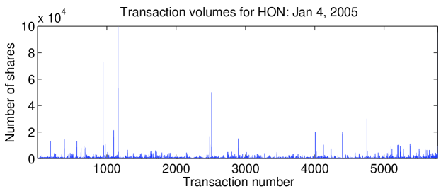
Figure 1: Transaction volumes for Honeywell Inc. (HON) from the NYSE and NASDAQ consolidated trades and quotes data base during January 4th, 2005. The observations correspond to the volumes (in a number shares) per single transaction. The transactions are listed in the order of their occurrence in time. The observed heavy–tailed behavior of traded volumes is ubiquitous across different trading days and across the entire spectrum of relatively liquid stocks.

The majority of the approaches proposed in the literature focuses on the scaling behavior of the largest order statistics $X_{(1)}\geq X_{(2)}\geq\cdots\geq X_{(n)}$ obtained from an in dependent and identically distributed (i.i.d.) sample $X(1),\ldots,X(n)$ from $F$; typical examples include Hill’s estimator hill:1975 and its numerous variations (kratz:resnick:1996, resnick:starica:1997), kernel based estimators (csorgo:deheuvels:mason:1985 and feuerverger:hall:1999). A review of these methods and their applications is given in dehaan:drees:resnick:2000 and desousa:michailidis:2004). The most widely used in practice is the Hill estimator $\widehat{\alpha}_{H}(k)$ defined as:

$$\widehat{\alpha}_{H}(k):={\Big{(}}\frac{1}{k}\sum_{i=1}^{k}\ln X_{(i)}-\ln X_{(k+1)}{\Big{)}}^{-1},$$ (1.3)

with $k,1\leq k\leq n-1$ being the number of included order statistics. The parameter $k$ is typically selected by examining the plot of the $\widehat{\alpha}_{H}(k)$’s versus $k$, known as the Hill plot. In practice, one chooses a value of $k$ where the Hill plot exhibits a fairly constant behavior (see e.g. dehaan:drees:resnick:2000). However, the use of order statistics requires sorting the data that is computationally expensive (requires at least $\mathcal{O}(n\log(n))$ steps) and destroys the time ordering of the data and hence their temporal structure. Further, as can be seen from the brief review above, most of the emphasis has been placed on point estimation of the tail index and little on constructing confidence intervals. Exceptions can be found in the work of cheng:peng:2001 and lu:peng:2002 for the construction of confidence intervals and of resnick:starica:1995 on the estimation of $\alpha$ for dependent data.

The purpose of this study is to introduce a method for estimating the tail index that overcomes the above listed shortcomings of other techniques. It is based on the asymptotic max self–similarity properties of heavy–tailed maxima. Specifically, the maximum values of data calculated over blocks of size $m$, scale at a rate of $m^{1/\alpha}$. Therefore, by examining a sequence of growing, dyadic block sizes $m=2^{j},\ 1\leq j\leq\log_{2}n,\ j\in{\mathbb{N}}$, and subsequently estimating the mean of logarithms of block–maxima (log–block–maxima) one obtains an estimate of the tail index $\alpha$. Notice that by using blocks of data, the temporal structure of the data is preserved. This procedure requires $\mathcal{O}(n)$ operations, making it particularly useful for large data sets; further, the estimates for $\alpha$ can be updated recursively as new data become available, by using only ${\mathcal{O}}(\log_{2}n)$ memory and without the knowledge of the entire data set, thus making the proposed estimator particularly suitable for streaming data. Estimators based on max–self similarity for the tail index for i.i.d. data were introduced in stoev:michailidis:taqqu:2006, where their consistency and asymptotic normality was established. In this paper, we extend them to dependent data, prove their consistency, examine and illustrate their performance using synthetic and real data sets and discuss a number of implementation issues.

The remainder of the paper is structured as follows: in Section 2 the max–spectrum estimators are introduced. Their consistency and asymptotic normality is established in Section 3.1, for $m-$dependent processes. The distributional consistency of the estimators is established in Section LABEL:s:d-cons for a large class of time series models (including linear processes) under a mild asymptotic independence condition. The construction of confidence intervals is further addressed in Section LABEL:s:conf_int. The important problem of automatic selection of parameters is addressed in Section LABEL:s:cut-off. Applications to financial time series are discussed in Section LABEL:s:data, while most technical proofs are given in the Appendix.

2 Max self–similarity and tail exponent estimators

Here we introduce the max self–similarity estimators for the tail exponent and demonstrate several of their characteristics. We start by reviewing the basic ideas for the case of independent and identically distributed (i.i.d.) data. A detailed exposition is given in stoev:michailidis:taqqu:2006.

Consider the sequence of block–maxima

$$X_{m}(k):=\max_{1\leq i\leq m}X(m(k-1)+i)=\bigvee_{i=1}^{m}X(m(k-1)+i),\ \ k=1,2,\ldots,~{}~{}m\in{\mathbb{N}},$$

where $X_{m}(k)$ denotes the largest observation in the $k-$th block. By (1.1) & (1.2) and the Fisher–Tippett–Gnedenko Theorem,

$${\Big{\{}}\frac{1}{m^{1/\alpha}}X_{m}(k){\Big{\}}}_{k\in{\mathbb{N}}}\stackrel{{\scriptstyle d}}{{\longrightarrow}}{\Big{\{}}Z(k){\Big{\}}}_{k\in{\mathbb{N}}},\ \ \ \mbox{ as }m\to\infty,$$ (2.1)

where $\stackrel{{\scriptstyle d}}{{\to}}$ denotes convergence of the finite–dimensional distributions, with the $Z(k)$’s being independent copies of an $\alpha-$Fréchet random variable. A random variable $Z$ is said to be $\alpha-$Fréchet, $\alpha>0$, with scale coefficient $\sigma>0$, if

$$\mathbb{P}\{Z\leq x\}=\left\{\begin{array}[]{ll}\exp\{-\sigma^{\alpha}x^{-\alpha}\}&,\ x>0\\ 0&,\ x\leq 0\end{array}\right.$$ (2.2)

The Fréchet variable $Z$ is said to be standard if $\sigma=1$.

Thus, for large $m$’s the block–maxima $X_{m}(k)$’s behave like a sequence of i.i.d. $\alpha-$Fréchet variables, which suggests the following:

Definition 2.1

A sequence of random variables $X=\{X(k)\}_{k\in{\mathbb{N}}}$ is said to be max self–similar with self–similarity parameter $H>0$, if for any $m>0$,

$${\{}\bigvee_{i=1}^{m}X(m(k-1)+i){\}}_{k\in{\mathbb{N}}}\stackrel{{\scriptstyle d}}{{=}}{\{}m^{H}X(k){\}}_{k\in{\mathbb{N}}},$$ (2.3)

with $=^{d}$ denoting equality of the finite–dimensional distributions.

Relationship (2.3) holds asymptotically for i.i.d. data and exactly for Fréchet distributed data. Hence, any sequence of i.i.d.  heavy–tailed variables can be regarded as asymptotically max self–similar with self–similarity parameter $H=1/\alpha$. This feature suggests that an estimator of $H$ and consequently $\alpha$ can be obtained by focusing on the scaling of the maximum values in blocks of growing size. A similar idea applied to block–wise sums was used in crovella:taqqu:1999 for estimating $\alpha$, in the case $0<\alpha<2$.

For an i.i.d.  sample $X(1),\ldots,X(n)$ from $F$, define

$$D(j,k):=\max_{1\leq i\leq 2^{j}}X(2^{j}(k-1)+i)=\bigvee_{i=1}^{2^{j}}X(2^{j}(k-1)+i),\ \ k=1,2,\ldots,n_{j},$$ (2.4)

for all $j=1,2,\ldots,[\log_{2}n],$ where $n_{j}:=[n/2^{j}]$ and where $[x]$ denotes the largest integer not greater than $x\in{\mathbb{R}}$. By analogy to the discrete wavelet transform, we refer to the parameter $j$ as the scale and to $k$ as the location parameter. We consider dyadic block–sizes because of their algorithmic and computational advantages. Introduce the statistics

$$Y_{j}:=\frac{1}{n_{j}}\sum_{k=1}^{n_{j}}\log_{2}D(j,k),\ \ j=1,2,\ldots,[\log_{2}n].$$ (2.5)

The Law of Large Numbers implies that for fixed $j$, as $n_{j}\to\infty$, the $Y_{j}$’s are consistent and unbiased estimators of $\mathbb{E}Y_{j}=\mathbb{E}\log_{2}D(j,1)$, if finite (see Corollary 3.1 in stoev:michailidis:taqqu:2006). On the other hand, the asymptotic max self–similarity (2.1) of $X$ and (2.4) suggest that under additional tail regularity conditions (see e.g. Proposition LABEL:p:moments below):

$$\mathbb{E}Y_{j}=\mathbb{E}\log_{2}D(j,1)\simeq jH+C\equiv j/\alpha+C,\ \ \ \mbox{ as }j\to\infty,$$ (2.6)

where $C=C(\sigma_{0},\alpha)=\mathbb{E}\log_{2}\sigma_{0}Z$, and where $\simeq$ means that the difference between the left– and the right–hand side tends to zero, with $Z$ being an $\alpha-$Fréchet variable with unit scale coefficient.

Then, a regression–based estimator of $H=1/\alpha$ (and hence $\alpha$) for a range of scales $1\leq j_{1}\leq j\leq j_{2}\leq[\log_{2}n]$ is given by:

$$\widehat{H}(j_{1},j_{2}):=\sum_{j=j_{1}}^{j_{2}}w_{j}Y_{j},\ \ \mbox{ and }\ \ \widehat{\alpha}(j_{1},j_{2}):=1/\widehat{H}(j_{1},j_{2}),$$ (2.7)

where the weights $w_{j}$’s are chosen so that $\sum_{j=j_{1}}^{j_{2}}w_{j}=0$ and $\sum_{j=j_{1}}^{j_{2}}jw_{j}=1$. The optimal weights $w_{j}$’s can be calculated through generalized least squares (GLS) regression using the asymptotic covariance matrix of the $Y_{j}$’s. In practice, it is important to at least use weighted least squares (WLS) regression to account for the difference in the variances of the $Y_{j}$’s (see, stoev:michailidis:taqqu:2006).

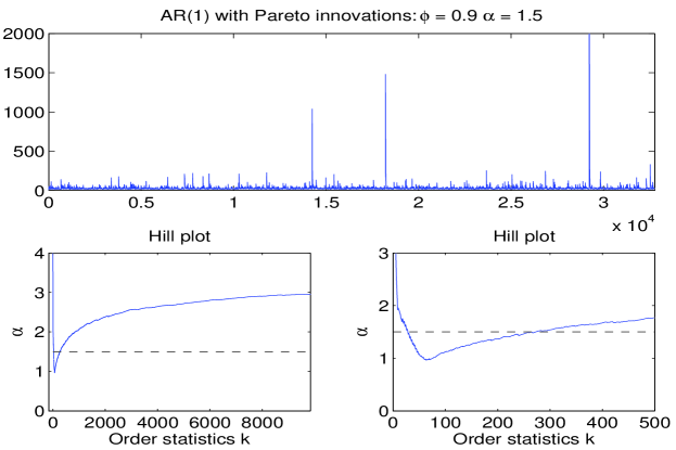
Figure 2: Top panel: auto–regressive time series of order 1 with Pareto innovations of tail exponent $\alpha=1.5$. Bottom left and right panels: the Hill plot for this data set and its zoomed–in version, respectively. The dashed horizontal line indicates the value of $\alpha=1.5$.

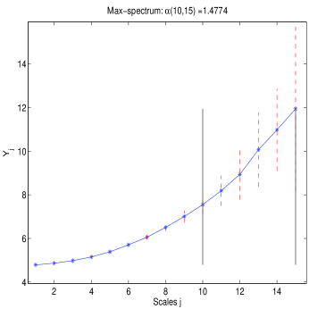
Figure 3: The max–spectrum plot for the data set in Figure 2. The max self–similarity estimator of the tail exponent, obtained from the range of scales $(j_{1},j_{2})=(10,15)$, is $\widehat{\alpha}(10,15)=1.4774$.

We propose to use the estimator defined in (2.7) for dependent time series data. We first illustrate its usage through a simulated data example. A data set of size $n=2^{15}=32,768$ was generated from an auto–regressive time series of order one with Pareto innovations. Specifically,

$$X(k)=\phi X(k-1)+Z(k)=\sum_{i=0}^{\infty}\phi^{i}Z(k-i),\ \ k=1,\ldots,n,$$

where $\phi=0.9$ and $\mathbb{P}\{Z(k)>x\}=x^{-\alpha},\ x>1$, with $\alpha=1.5$. The data together with its Hill plot are shown in Figure 2. Notice that even though the Hill estimator work best for Pareto data, the dependence structure in the model leads to a Hill plot, which is substantially different from that for independent Pareto data (see the bottom left panel). The zoomed–in version of the Hill plot (bottom right panel) however indicates that the tail exponent should be in the range between $1$ and $2$. The choices of $k$ in the range between $200$ and $400$ do in fact lead to estimates around $1.5$. This range however is hard to guess if one did not know the true value of $\alpha=1.5$. resnick:starica:1997 have shown that the Hill estimator is consistent for such dependent data sets. Nevertheless, as this example indicates, the Hill plot can be difficult to assess in practice.

In Figure 3, the max–spectrum plot is shown; i.e. the plot of the statistics $Y_{j}$ versus the available dyadic scales $j,~{}1\leq j\leq[\log_{2}n](=15)$. The estimated tail exponent over the range of scales $(10,15)$ is $1.4774$, which is very close to the nominal value of $\alpha=1.5$. Moreover, the max–spectrum is easy to assess and interpret. One sees a “knee” in the plot near scale $j=10$, where the max–spectrum curves upwards and thus it is natural to choose the range of scales $(10,15)$ to estimate $\alpha$. The choice of the scales $(j_{1},j_{2})$ can be also automated, as briefly discussed in Section LABEL:s:cut-off below.

Remark: (on the algorithmic implementation) The max–spectrum $Y_{j},\ j=1,\ldots,[\log_{2}n]$ of a data set $X_{1},\ldots,X_{n}$ can be computed efficiently in ${\mathcal{O}}(n)$ steps, without sorting the data. Indeed, this is evident from the recursive construction of block maxima, since

$$D(j+1,k)=\max\{D(j,2k-1),D(j,2k)\},\ \ k=1,\ldots,[n/2^{j+1}],\ \ 1\leq j<[\log_{2}n].$$

Moreover, this property can be further used to obtain a sequential algorithm for the computation of the $Y_{j}$’s. Indeed, keep in addition to the $Y_{j}$’s, the last block–maximum $D_{j}:=D(j,n_{j}),\ n_{j}=[n/2^{j}]$ per scale $j$, and also the extra variables $R_{j}=\max_{2^{j}n_{j}<i\leq n}X(i)$, which represent the maxima of the ’left–over’ $X_{i}$’s over the range $2^{j}[n/2^{j}]<i\leq n$. Now, if a new observation $X_{n+1}$ is recorded, one can easily update the $R_{j}$’s and the $Y_{j}$’s, with the help of the $R_{j}$’s, and the $D_{j^{\prime}}:=D(j^{\prime},n_{j^{\prime}})$’s, for $1\leq j^{\prime}<j$. Thus, one recovers the $(Y_{j},D_{j},R_{j})_{j}-$representation of the data $X_{1},\ldots,X_{n+1}$. Since only $\log_{2}n$ scales are available, we perform ${\mathcal{O}}(\log_{2}n)$ operations per update and use ${\mathcal{O}}(\log_{2}n)$ memory to store the max–spectrum and the auxiliary data.

This sequential implementation of the max–spectrum is of critical importance in the context of data streams in modern data bases or Internet traffic applications. In such settings, large volumes of data are observed in short amounts of time; they cannot be stored and/or sorted efficiently while at the same time rapid ’queries’ need to be answered about various statistics of the data. The proposed max–spectrum estimator provides a unique tool for the estimation of the tail–exponent of such data. Notice that the other available techniques require sorting the data which is impossible without having to store the entire data set. A sequential implementation of the Hill estimator for example would require ${\mathcal{O}}(n)$ memory, which is prohibitive in many applications.

3 Asymptotic properties

3.1 Asymptotic Normality (in the intermediate scales regime)

The estimators $\widehat{H}$ and $\widehat{\alpha}=1/\widehat{H}$ in (2.7) utilize the scaling properties of the max–spectrum statistics $Y_{j}$ in (2.5). The discussion in Section 2 suggests that the max self–similarity estimators in (2.7) will be consistent as both the scale $j$ and $n_{j}$ tend to infinity. The consistency and asymptotic normality of these estimators was established in stoev:michailidis:taqqu:2006 for i.i.d. data. This was accomplished by assessing the rate of convergence of moment type functionals of block–maxima, such as $\mathbb{E}\log_{2}D(j,1)$, under mild conditions on the rate of the tail decay in (1.1). Here, we focus on the case of dependent data and establish the asymptotic normality of the proposed max self–similarity estimators under analogous conditions on the rate.

Consider a strictly stationary process (time series) $X=\{X(k)\}_{k\in{\mathbb{Z}}}$ with heavy–tailed marginal c.d.f. $F$ as in (1.1) & (1.2). Further, assume that the $X(i)$’s are positive, almost surely, that is, $F(0)=0$. In many contexts, the block–maxima of $X$ scale at a rate $m^{1/\alpha}$ as the block size $m$ grows even under the presence of strong dependence. This is so, for example, when the time series $X$ has a positive extremal index (see, p. 53 in leadbetter:lindgren:rootzen:1983). The following conditions make this more precise by quantifying further the rate of convergence.

Let $M_{n}:=\max_{1\leq k\leq n}X(k)$ and let

$$F_{n}(x)\equiv\mathbb{P}\{M_{n}/n^{1/\alpha}\leq x\}=:\exp\{-c(n,x)x^{-\alpha}\},\ \ \ x>0,\ \ n\in{\mathbb{N}}.$$

One can see that $M_{n}/n^{1/\alpha}\stackrel{{\scriptstyle d}}{{\longrightarrow}}Z,\ n\to\infty$ if and only if $c(n,x)\to c_{X}\equiv\mbox{\rm const}\,,\ n\to\infty,$ for all $x>0$, where $Z$ is an $\alpha-$Fréchet variable with scale $\sigma=c_{X}^{1/\alpha}$. The following conditions will help us quantify the rate of the last convergence and also obtain rates of convergence for moment functionals of block–maxima in Proposition 3.1 below.

Condition 3.1

There exists $\beta>0$ and $R\in{\mathbb{R}}$, such that

$$|c(n,x)-c_{X}|\leq c_{1}(x)n^{-\beta},\ \ \mbox{ for all }x>0,\ \ \ \ \mbox{ and }\ \ \ c_{1}(x)={\mathcal{O}}(x^{-R}),\ x\downarrow 0,$$ (3.1)

for some $c_{X}>0$.

Condition 3.2

For all $x>0$, we have

$$c(n,x)\geq c_{2}\min\{1,x^{\gamma}\},\ \ \mbox{ for some }\gamma\in(0,\alpha),$$ (3.2)

for all sufficiently large $n\in\mathbb{N}$, where $c_{2}>0$ does not depend on $n$.

Remarks

1. Conditions 3.1 and 3.2 are not very restrictive. They can be shown to hold, for example, for a large class of moving maxima processes (see, Proposition LABEL:p:m_max).

2. Condition 3.1 implies in particular that $M_{n}/n^{1/\alpha}\stackrel{{\scriptstyle d}}{{\to}}c_{X}^{1/\alpha}Z,$ as $n\to\infty$, for a standard $\alpha-$Fréchet variable $Z$. In view of (1.1), we also have that $M_{n}^{*}/n^{1/\alpha}\stackrel{{\scriptstyle d}}{{\to}}\sigma_{0}Z$, as $n\to\infty$, with $M_{n}^{*}:=\max_{1\leq k\leq n}X(k)^{*}$, where the $X(k)^{*}$’s are i.i.d. random variables with c.d.f. $F$. This implies that the extremal index $\theta$ of the time series $X$ is: $\theta:=c_{X}/\sigma_{0}^{\alpha}$ (see, e.g. p. 53 in leadbetter:lindgren:rootzen:1983).

Conditions 3.1 & 3.2, yield the following important result on the rate of convergence of log–block maxima, similar to Corollary 3.1 in stoev:michailidis:taqqu:2006.

Proposition 3.1

Let $X=\{X(k)\}_{k\in\mathbb{Z}}$ be a strictly stationary time series which satisfies Conditions 3.1 & 3.2. Suppose that $\int_{1}^{\infty}c_{1}(x)x^{-\alpha-1+\delta}dx<\infty$, for some $\delta>0$. Then, with $M_{n}:=\max_{1\leq k\leq n}X_{k}$, we have $\mathbb{E}|\ln(M_{n})|^{p}<\infty$, for all $p>0$ and all sufficiently large $n\in{\mathbb{N}}$. Moreover, for any $p>0$ and $k\in{\mathbb{N}}$, we have:

$${\Big{|}}\mathbb{E}|\ln(M_{n}/n^{1/\alpha})|^{p}-\mathbb{E}|\ln(Z)|^{p}{\Big{|}}={\mathcal{O}}(n^{-\beta}),\ \ \mbox{ and }\ \ {\Big{|}}\mathbb{E}(\ln(M_{n}/n^{1/\alpha}))^{k}-\mathbb{E}(\ln(Z))^{k}{\Big{|}}={\mathcal{O}}(n^{-\beta}),$$

as $n\to\infty$, where $Z$ is an $\alpha-$Fréchet random variable with scale coefficient $\sigma=c_{X}^{1/\alpha}$.

The proof is given in Section LABEL:s:proofs. Proposition 3.1 readily implies:

$$\mathbb{E}(Y_{j}-j/\alpha)\equiv\mathbb{E}\log_{2}(D(j,k)/2^{j/\alpha})=\mathbb{E}\log_{2}(c_{X}^{1/\alpha}Z_{1})+{\mathcal{O}}(1/2^{j\beta}),$$ (3.3)

as $j\to\infty$, where $Z_{1}$ is a standard $\alpha-$Fréchet variable. This result yields an asymptotic bound on the bias of the estimators $\widehat{H}(j_{1},j_{2})$ in (2.7) above.

Proposition 3.1 can be further used to establish the asymptotic normality of $\widehat{\alpha}(j_{1},j_{2})=1/\widehat{H}(j_{1},j_{2})$ in (2.7). To do so, we focus on a range of scales $(j_{1},j_{2})$ which grows with the sample size. Namely, we fix $\ell\in{\mathbb{N}},\ \ell\geq 2$, let $j_{1}:=1+j(n)$ & $j_{2}:=\ell+j(n)$, and as in (2.7) define:

$$\widehat{H}_{n}:=\sum_{i=1}^{\ell}w_{i}Y_{i+j(n)}\ \ \ \mbox{ and }\ \ \ \widehat{\alpha}_{n}:=1/\widehat{H}_{n},$$

where $\sum_{i=0}^{\ell-1}i^{\kappa}w_{i}=\kappa,\ \kappa=0,1$. The next theorem is the main result of this section. It establishes the asymptotic normality of the estimator $\widehat{\alpha}_{n}$, as $j(n)$ and $n$ tend to infinity.

Theorem 3.1

Let $X_{1},\ldots,X_{n}$ be a sample from an $m-$dependent heavy–tailed process $X=\{X(k)\}_{k\in{\mathbb{Z}}}$. Suppose that (3.1) and (3.2) hold and let $j=j(n)\in{\mathbb{N}}$ be such that

$$2^{j(n)}/n+n/2^{j(n)(1+2\min\{1,\beta\})}\longrightarrow 0,\ \ \ \mbox{ as }n\to\infty.$$ (3.4)

Then, as $n\to\infty$,

$$\sqrt{n_{j}}(\widehat{\alpha}_{n}-\alpha)\stackrel{{\scriptstyle d}}{{\longrightarrow}}{\mathcal{N}}(0,\alpha^{2}c_{w}),\ \ \ \mbox{ with }c_{w}=\sum_{i^{\prime},i^{\prime\prime}=1}^{\ell}w_{i^{\prime}}w_{i^{\prime\prime}}\Sigma_{1}(i^{\prime},i^{\prime\prime}),$$ (3.5)

where $n_{j}=[n/2^{j}]$. Here $\Sigma_{1}(i^{\prime},i^{\prime\prime})=2^{\min\{i^{\prime},i^{\prime\prime}\}}{\rm Cov}(\log_{2}Z_{1},\log_{2}(Z_{1}\vee(2^{|i^{\prime}-i^{\prime\prime}|}-1)Z_{2})),$ for $i^{\prime},i^{\prime\prime}=1,\ldots,\ell$, where $Z_{1}$ and $Z_{2}$ are independent standard $1-$Fréchet random variables.