VLT multi-object spectroscopy of 33 eclipsing binaries in the Small Magellanic Cloud

Abstract

Aims. Our purpose is to provide reliable stellar parameters for a significant sample of eclipsing binaries, which are representative of a whole dwarf and metal-poor galaxy. We also aim at providing a new estimate of the mean distance to the SMC and of its depth along the line of sight for the observed field of view.

Methods. We use radial velocity curves obtained with the ESO FLAMES facility at the VLT and light curves from the OGLE-II photometric survey. The radial velocities were obtained by least-squares fits of the observed spectra to synthetic ones, excluding the hydrogen Balmer lines.

Results. Our sample contains 23 detached, 9 semi-detached and 1 overcontact systems. Most detached systems have properties consistent with stellar evolution calculations from single-star models at the standard SMC metallicity $Z=0.004$, though they tend to be slightly overluminous. The few exceptions are probably due to third light contribution or insufficient signal-to-noise ratio. The mass ratios are consistent with a flat distribution, both for detached and semi-detached/contact binaries. A mass-luminosity relation valid from $\sim$4 to $\sim$18 $\mathcal{M}_{\odot}$ is derived. The uncertainties are in the $\pm$2 to $\pm$11 % range for the masses, in the $\pm$2 to $\pm$5 % range for the radii and in the $\pm$1 to $\pm$6 % range for the effective temperatures. The average distance modulus is $19.11\pm 0.03$ ($66.4\pm 0.9$ kpc). The moduli derived from the $V$ and from the $I$ data are consistent within $0.01$ mag. The $2\,\sigma$ depth of the SMC is, for our field, of $0.25$ mag or $7.6$ kpc under the assumption of a gaussian distribution of stars along the line of sight. Three systems show significant apsidal motion, one of them with an apsidal period of 7.6 years, the shortest known to date for a detached system with main sequence stars.

1 Introduction

Since the late 1990s, the usefulness of extragalactic eclipsing binaries has been emphasized in a number of papers. The reader can notably refer to the excellent reviews from Clausen (jC04 (2004)) and Guinan (eG04 (2004), eG07 (2007)). The two major contributions of eclipsing binaries (hereafter EBs) to astrophysics are to provide (1) fundamental mass and radius measurements for the component stars, allowing to test stellar evolution models, and (2) precise distance moduli (DMi) derived from the luminosities calculated from the combination of the absolute radii with the effective temperatures. Until a purely geometrical distance determination is feasible, Paczyński (bP01 (2001)) considers that detached EBs are the most promising distance indicators to the Magellanic Clouds. Besides, Wyithe & Wilson (WW02 (2002), hereafter WW02) remarked that semi-detached EBs are even more promising, since their parameters are better constrained.

The renewal of interest in extragalactic EBs, especially EBs in the Magellanic Clouds, has been stimulated by the release of a huge number of light curves as a byproduct of automated microlensing surveys (EROS, MACHO, OGLE) with 1-m class telescopes. As photometry is only half of the story, high resolution spectrographs attached to 4-m class or larger telescopes had to be used to obtain reliable radial velocity (RV) curves. Four B-type EB systems belonging to the Large Magellanic Cloud (LMC) were accurately characterized in a series of papers from Guinan et al. (GFD98 (1998)), Ribas et al. (RGF00 (2000), RFMGU02 (2002)) and Fitzpatrick et al. (FRG02 (2002), FRGMC03 (2003)). More recently, from high resolution, high $S/N$ spectra obtained with UVES at the ESO VLT, the analysis of eight more LMC systems was presented by González et al. (GOMM05 (2005)). A corner stone in the study of EBs in the SMC was set up with the release of two papers from Harries et al. (HHH03 (2003), hereinafter HHH03) and Hilditch et al. (HHH05 (2005), hereinafter HHH05) giving the fundamental parameters of a total of 50 EB systems of spectral types O and B. The spectroscopic data were obtained with the 2dF multi-object spectrograph on the 3.9-m Anglo-Australian Telescope. To our knowledge this is the first use of multi-object spectroscopy in the field of extragalactic EBs. Recently, even the distance to large spiral galaxies were measured on the basis of two EBs in M31 (Ribas et al. RJVFHG05 (2005), Vilardell et al. Vil10 (2010)) and one in M33 (Bonanos et al. BSK06 (2006)).

The huge asymmetry, between the number of EB light curves published so far and the very small number of RV curves, is striking. If one considers the SMC, the new OGLE-II catalog of EBs in the SMC (Wyrzykowski et al. 2004) contains 1350 light curves and currently only 50 of these systems have moderately reliable RV curves. This paper reduces a little this imbalance by releasing the analysis of 28 more EB systems plus revised solutions for 5 systems previously described by HHH03 and HHH05. The RV measurements were derived from muti-object spectroscopic observations made with the VLT FLAMES facility.

Another strong motivation for increasing the number of fully resolved binaries is to settle the problem of the distribution of the mass ratio of detached binaries with early B primaries. Recently, two papers were published supporting two diametrically opposed conclusions: van Rensbergen et al. (VDJ06 (2006)), whose work is based on the 9th Catalogue of Spectroscopic Binaries (Pourbaix et al. PTB04 (2004)), support the view that the $q$-distribution (where $q$ is the mass ratio) follows a Salpeter-like decreasing power law; however, from the examination of the homogeneous sample of the 21 detached systems characterized by HHH03 and HHH05, Pinsonneault & Stanek (PS06 (2006)) draw the conclusion that the proportion of close detached systems with mass ratio $q>0.87$ far outnumbers what can be expected from either a Salpeter or a flat $q$-distribution (the “twins” hypothesis). Finally, let us mention that the $q$-distribution of semi-detached (i.e. evolved) systems is no more settled, the statistics strongly depending on the method used to find the mass ratios, i.e. from the light curve solution or from SB2 spectra (van Rensbergen et al. VDJ06 (2006)).

Although the controversy about the characteristic distance to the SMC seems to be solved in favour of a mid position between the “short” and the “long” scales, distance data and line of sight depth remain vital for comparison with theoretical models concerning the three-dimensional structure and the kinematics of the SMC (Stanimirović et al. SSJ04 (2004)).

Our contribution provides both qualitative and quantitative improvements over previous studies. Thanks to the VLT GIRAFFE facility, spectra were obtained with a resolution three times that in HHH03/05’s study. Another strong point is the treatment of nebular emission. The SMC is known to be rich in H ii regions (Fitzpatrick elF85 (1985), Torres & Carranza TC87 (1987)). Consequently, strong Balmer lines in emission are very often present in the spectra of the binary systems under study. Therefore, it appeared rapidly that it was essential to find a consistent way to deal with this “third component” polluting most double-lined (SB2) spectra.

We present the observations in Section 2. The reduction of the spectroscopic data and the interpretation of both photometric and spectroscopic data are described in Section 3, where the errors are also discussed in detail. The individual binary systems are described in Section 4, while the sample as a whole is discussed in relation with the SMC properties in Section 5.

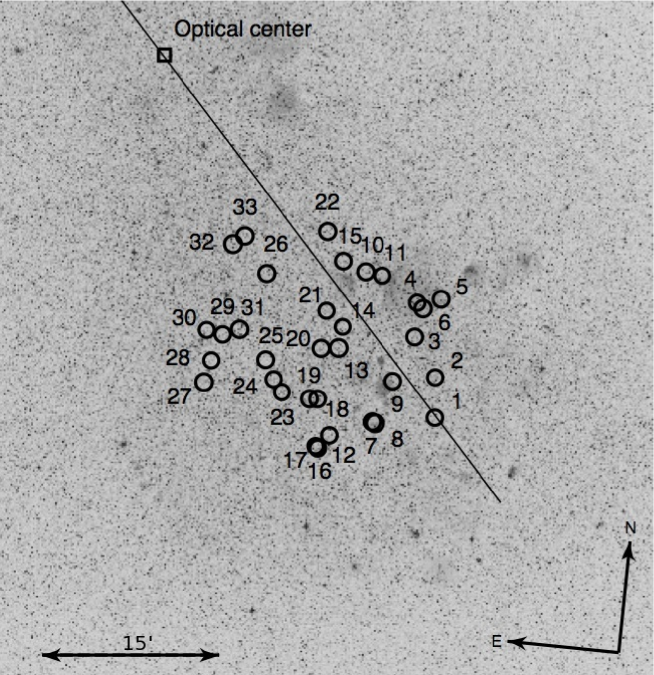
Figure 1: Positions of the 33 binaries in the 1$\degr$ $\times$ 1$\degr$ surrounding field centered on (J2000) $00^{\mathrm{h}}49^{\mathrm{m}}20^{\mathrm{s}}$, $-73\degr 13\arcmin 37.3\arcsec$. They lie alongside the southwestern part of the SMC bar (oblique line) at $\sim$0.5$\degr$ of the SMC optical center. Image retrieved from the STScI Digitized Sky Survey (POSS-II/UK Schmidt Telescope, Red) (copyright ©1993-5 Anglo-Australian Observatory.)

2 Observations

The targets, astrometry included, were selected from the first OGLE photometric catalog. The GIRAFFE field of view (FoV) constrained to choose systems inside a 25′-diameter circle. Other constraints were $I\leq 18$ mag, at least 15 well-behaved detached light curves (for the SMC field) and finally seven bump cepheids in the FoV (for another program). The positions in the sky of 33 objects studied in this paper are shown in Fig. 1. The epoch, exposure time, air mass, seeing and age of moon for each of the 16 CCD frames are gathered in Table 1.

The relation between our own 1–33 labeling and the OGLE names can be found in Table 3, which lists the basic parameters of the systems. The coordinates are from Wyrzykowski et al. (WUK04 (2004)). The orbital periods and epochs of the primary minimum are close to those listed by Wyrzykowski et al. (WUK04 (2004)), but the periods were improved as far as possible using the radial velocity curves determined in this work. That was worth the effort, since spectroscopic observations were performed more than three years after the last photometric ones. Since the times of the photometric minima are quite sharply defined, the uncertainty on the period (mentioned between parentheses in Table 3) is based on the uncertainty of the spectroscopically defined epoch of the primary minimum. The latter is quite precise for circular orbits; for eccentric orbits, it is less accurate, because the Kepler equation had to be solved and the solution is affected by the uncertainty on the eccentricity. We have decided here to adopt the dynamic definition of the primary and secondary components, rather than the photometric one. In other words, the primary component is always the more massive one, and the primary minimum always corresponds to the eclipse of the primary by the secondary component. As a consequence, it may happen that the so-called primary minimum is not the deeper one. Figure 2 shows the histogram of the periods. The strong observational bias in favour of short periods is conspicuous.

For all but two binaries, the light curves come from the new version of the OGLE-II catalog of eclipsing binaries detected in the SMC (Wyrzykowski et al. WUK04 (2004)). This catalog is based on the Difference Image Analysis (DIA) catalog of variable stars in the SMC (see http://sirius.astrouw.edu.pl/$\sim$ogle/ogle2/ smc_ecl/index.html). The data were collected from 1997 to 2000. The systems 4 121084 and 5 100731 were selected from the first version of the catalog (standard PSF photometry) but for an unknow reason they do no appear anymore in the new version. Nevertheless, they were retained as there is no objective reason to exclude them.

The DIA photometry is based on $I$-band observations (between 202 and 312 points per curve). $B$ and $V$ light curves were also used in spite of a much poorer sampling (between 22–28 points/curve and 28–46 points/curve in $B$ and $V$ respectively). To give an idea of the accuracy of the OGLE photometry, the objects studied in this paper have an average $I$ magnitude and scatter in the range $15.083\pm 0.009$ to $18.159\pm 0.047$. These values were calculated from the best-fitting synthetic light curves. For the two other bands, we get $14.701\pm 0.011$ to $18.090\pm 0.025$ for $B$ and $14.966\pm 0.009$ to $18.173\pm 0.023$ for $V$. The quality of an observed light curve can be better expressed by comparing the depth of the primary minimum $\Delta I_{\mathrm{minI}}$ to the average RMS scatter $\sigma_{I}$. These ratios are shown in Table 16. This permits to classify the light curves in five categories: low ($\Delta I_{\mathrm{minI}}/\sigma_{I}<10$), low-to-medium ($10\leq\Delta I_{\mathrm{minI}}/\sigma_{I}<20$), medium ($20\leq\Delta I_{\mathrm{minI}}/\sigma_{I}<30$), medium-to-high ($30\leq\Delta I_{\mathrm{minI}}/\sigma_{I}<40$) and high ($\Delta I_{\mathrm{minI}}/\sigma_{I}\geq 40$) quality. According to this scheme, most $I-$band light curves (58%) belong to the low-to-medium and medium quality categories, one-third (33%) in the medium-to-high and high quality categories, and the remaining 9% in the poor quality category. This classification scheme is not useful for the other bands, the low sampling being the limiting factor.

VLT FLAMES/GIRAFFE spectroscopy was obtained by one of us (FR) during eight consecutive nights from November 16 to 23, 2003. The spectrograph was used in the low resolution (LR2) Medusa mode: resolving power $R=6400$, bandwidth $\Delta\lambda=603$ Å centered on $4272$ Å. The most prominent absorption lines in the blue part of early-B stars spectra are: H$\epsilon$, He i $\lambda 4026$, H$\delta$, He i $\lambda 4144$, H$\gamma$, He i $\lambda 4388$, and He i $\lambda 4471$. For late-O stars, He ii $\lambda 4200$ and He ii $\lambda 4542$ gain in importance. Two fields, one in the SMC and one in the LMC, were alternatively observed at a rate of four exposures per night with an integration time of 2595 s for all but one epoch. Therefore, 16 spectra per target were obtained, with a total of 104 targets in the SMC and 44 in the LMC. The LMC SB2 systems are being analyzed and will be presented in another paper.

Beside the spectra of the objects, 21 sky spectra were obtained for each exposure in the SMC. The parameters related to the spectroscopic observations are gathered in Table 1. The observed signal-to-noise ratios ($S/N$) were determined for each smoothed spectrum (see Section 3.1) in the continuum between 4195 and 4240 Å. For each object, two values are presented in Table 11: the highest and lowest $S/N$ values for an exposure of 2595 s. Not surprisingly, the short exposure of 707 s (due to a technical problem) was useful for the brightest objects only. For a given binary with $t_{\mathrm{exp}}=2595$ s, the ratio of the highest $S/N$ to the lowest $S/N$ is $\sim$2.

Table 1: Spectroscopic observations: epochs, heliocentric Julian dates, exposure times and sky conditions. The value of the air mass is given at mid exposure. The value of the seeing is an average between the start and end values. The moon age is the number of days elapsed since the last new moon.

Date of observation (start)	HJD	$t_{\mathrm{exp}}$	Air mass	Seeing	Age of Moon
	($-$2 450 000)	(s)		($\arcsec$)	(d)
2003-11-16T00:39:59.373	2959.5423	2595	1.526	0.77	21.00
2003-11-16T04:43:39.664	2959.7115	2595	1.744	0.53	21.16
2003-11-17T00:35:51.283	2960.5394	2595	1.526	1.27	21.96
2003-11-17T03:55:11.067	2960.6778	2595	1.645	0.95	22.09
2003-11-18T00:27:41.157	2961.5336	2595	1.529	0.80	22.94
2003-11-18T04:40:08.506	2961.7090	2595	1.755	0.96	23.12
2003-11-19T00:41:56.657	2962.5435	2595	1.519	1.00	23.97
2003-11-19T05:06:05.545	2962.7269	2595	1.845	0.67	24.16
2003-11-20T00:27:32.704	2963.5335	2595	1.524	1.01	25.02
2003-11-21T00:46:40.291	2964.5358	707	1.518	0.98	26.13
2003-11-21T01:00:00.631	2964.5560	2595	1.512	0.83	26.14
2003-11-21T05:39:31.454	2964.7501	2595	1.998	0.74	26.35
2003-11-22T00:20:45.386	2965.5287	2595	1.523	0.94	27.23
2003-11-22T04:32:44.400	2965.7037	2595	1.779	0.92	27.43
2003-11-23T00:44:54.938	2966.5454	2594	1.514	0.68	28.40
2003-11-23T04:27:51.663	2966.7002	2595	1.778	1.02	28.58

3 Data reductions and analysis

3.1 Spectroscopic data reduction

The basic reduction and calibration steps including velocity correction to the heliocentric reference frame for the spectra were performed with the GIRAFFE Base Line Data Reduction Software (BLDRS) (see http://girbldrs.sourceforge.net). Sky subtraction, a critical step for faint objects, was done as follows: for each epoch an average sky spectrum was computed from the 21 sky spectra measured over the whole FoV. For a given epoch the sky level was found to vary slightly across the field, but interpolating between spectra was not considered a valuable alternative. Local sky variations with respect to the average spectrum are given in Table 8. The values $\Delta_{\mathrm{sky}}$ are read as follows: for example, the sky position labeled S19 is on average (i.e. over all epochs) $\sim$20% brighter than the mean (i.e. over all sky positions) sky spectrum. The variations were found to be between about $-11$ and $+35$%. Normalization to the continuum, cosmic-rays removal and Gaussian smoothing ($FWHM$ = 3.3 pix) were performed with standard NOAO/PyRAF tasks.

The first 60 Å of the spectra, i.e for wavelengths between 3940 and 4000 Å, were suppressed. The reason is that below $\sim$4000Å the $S/N$ is getting very poor and therefore there is no reliable way to place the continuum. Furthermore, the region around H$\epsilon$ was found to be strongly contaminated by the interstellar Ca ii H and K absorption lines. The last few  Å (above 4565 Å) were equally found unusable because of a strongly corrupted signal.

Figure 2: Histogram of periods of our sample of 33 eclipsing binaries in 0.5 day bins.

3.2 Analysis

For historical reasons, the analysis has been made in essentially two steps.

First, RG did a complete analysis of all systems, using the KOREL code (Hadrava pH95 (1995), pH04 (2004)) to obtain both the radial velocity curves and the disentangled spectra of the individual components. Then, the simultaneous analysis of light and RV curves was made with the 2003 version of the Wilson-Devinney (WD) Binary Star Observables Program (Wilson & Devinney WD71 (1971); Wilson rW79 (1979), rW90 (1990)) via the PHOEBE interface (Prša & Zwitter PZ05 (2005)). However, simulations performed following the referee’s request regarding this early version of the work, showed that the amplitude $K_{\mathrm{P}}$ of the RV curve and the mass ratio $q\equiv\mathcal{M}_{\mathrm{S}}/\mathcal{M}_{\mathrm{P}}=K_{\mathrm{P}}/K_{\mathrm{S}}$ were not recovered with the expected robustness. More details about these simulations are given below (Section 3.5.1). Although, on average, the right values are recovered, one particular solution may be off by as much as five percent (one sigma) or ten percent (two sigma), which was deemed unsatisfactory.

Thus, a second, almost independent analysis was made by PN, using a least-squares fit of synthetic binary spectra to observed unsmoothed spectra for the RV determinations. The latter technique seemed much more robust, according to the same simulation: the $K_{\mathrm{P}}$ and $K_{\mathrm{S}}$ amplitudes are recovered to better than one percent – at least for the particular binary that was simulated – and the dispersion of the values of the small eccentricity ($e\sim 0.03$) is no larger than two percent. Small systematic errors may result from temperature or rotation mismatch, but they remain smaller than the uncertainties of the previous analysis.

We took the opportunity of this new analysis to define a more objective determination of the effective temperatures of the components. Instead of a visual fit of a spectrum close to quadrature, we used a least-squares fit of synthetic binary spectra to all observed spectra falling out of eclipses. Then, the error on the effective temperatures could be naturally defined as the RMS scatter of the results. More details are given in the next sections and in the following discussion of individual binaries.

3.3 Photometry: quality check

The quality of the $I-$band light curves was discussed in Section 2. Despite the high range of RMS scatter, we can expect a very accurate determination of the out-of-eclipse $I-$magnitude because of the large number of data points ($\sim$300). This is not the case with the $B-$ and $V-$bands. A much poorer sampling can lead to erroneous zero-level computation in the light-curve analysis step and result in wrong colour-index determination. Therefore, it is necessary to perform a quality check of the photometric data. This was done in the form of colour-colour diagrams of our sample. Figure 3 presents the three diagrams that can be obtained from the three colour indices $(B-V)^{\mathrm{q}}$, $(V-I)^{\mathrm{q}}$ and $(B-I)^{\mathrm{q}}$. These are the values at quadratures, i.e an average value characterizing a “hybrid” star of intermediate properties with respect to the two components of a particular system. Not surprisingly, most binaries are found on a relatively narrow linear strip. For any diagram, the scatter of the objects is low because the reddening line is almost parallel to the sequence. For example, the ratio $E_{B-V}/E_{V-I}=0.81$, determined from Eq. 11 in Section 3.12, is close to 0.69, the slope of the sequence $(B-V)^{\mathrm{q}}$ vs. $(V-I)^{\mathrm{q}}$. Nevertheless, four outliers appear, which are marked with open symbols. In principle, there is a possibility to restore a bad colour index, as illustrated by the example of the system 5 261267: Inspecting the three light curves, one can suspect that the cause of the discrepancy lies in a poorly sampled $V-$band light curve in the out-of-eclipse domain. The other two light curves ($B$ and $I$) seem more reliable. Therefore, only the $B-I$ colour-index is reliable for this system. But the two other indices, $B-V$ and $V-I$, can safely be interpolated from the $B-I$ value under the assumption that the system lies on the linear strip. The method is illustrated by the dashed lines in the diagrams. Of course, this reconstruction of two bad indices from a good one is not possible, unless only one of the three light curves is unreliable (either $B$ or $V$). In this particular example, the situation is not so clear-cut because the reconstructed indices ($B-V=-0.129$ and $V-I=-0.139$) would imply too low a $V^{q}$ value. Therefore, all four outliers will be excluded in the final estimate of the distance modulus.

On the upper right diagram of Fig. 3, red crosses indicate the intrinsic colours computed below (Section 3.11). Their positions, slightly below the regression line of the sequence, is entirely compatible with the reddening arrow and the observed colours, which inspires confidence regarding the colour excesses determined in Section 3.11.

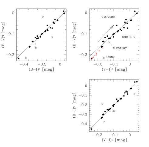
Figure 3: Observed (reddened) colour-colour diagrams of our sample. These are the brightest out-of-eclipse values from Table 3. They were determined from the best light-curve fits. The low scatter is due to a reddening line almost parallel to the main sequence (see upper right panel). Note that some values (open symbol) are doubtful as they lie off the linear trend. The dashed lines illustrate how to recover correct $B-V$ and $V-I$ indices from doubtful ones, under the assumption that the $B-I$ index is reliable, for the system 5 261267.

3.4 Synthetic spectra

Except for the first two steps of the analysis, i.e. (a) the simultaneous disentangling of the composite spectra and retrieving of the RV curves through the KOREL code (Hadrava pH95 (1995), pH04 (2004)) and (b) the simultaneous analysis of the light and RV curves through the WD/PHOEBE code, the search for the parameters of a binary relies heavily on synthetic spectra. Indeed, the systemic velocity, the projected rotational velocities, the ratio of radii and the primary temperature are found by comparing the observed spectra (disentangled and composite as well) with a library of synthetic spectra. Actually, two libraries were used. For objects with effective temperature $15\,000\ \mathrm{K}\leq T_{\mathrm{eff}}\leq 30\,000\ \mathrm{K}$, we used the BSTAR2006 library recently released by Lanz & Hubeny (LH07 (2007)). For the few objects above $30\,000\ \mathrm{K}$, we took the OSTAR2002 library previously released by the same authors (LH03 (2003)). Both libraries are available at the TLUSTY Web site (verb+http://nova.astro.umd.edu/index.html+).

The grids with a metallicity suitable for the SMC, $Z=0.004$, i.e. one-fifth of the solar metallicity, were chosen. Concerning the BSTAR2006 library, we took the grid with a microturbulent velocity of 2 km s^-1. Both grids of spectra are based on NLTE line-blanketed model atmospheres. The temperature step is 1000 K below $30\,000\ \mathrm{K}$ and 2500 K for early-O stars. We restrained to surface gravities $3.25\ \mathrm{dex}\leq\log g\leq 4.75\ \mathrm{dex}$ (0.25 dex step) . The spectra were convolved with the appropriate rotational profiles ($V_{\mathrm{rot}}\sin i$ = 30, 40, 50, 75, 100, 150, 200, 250 and 300 km s^-1) and with a Gaussian instrumental profile (resolution of 0.67 Å) by mean of the program ROTIN3 (http://nova.astro.umd.edu/Synspec43/synspec-frames-rotin.html). Beside a grid of continuum normalized spectra, a grid of flux spectra was generated for colour indices calculation through synthetic photometry.

Formally, a normalized synthetic composite spectrum is computed at a given orbital phase $\phi$ from the normalized $j-$component spectra $F^{\mathrm{n}}_{j,c\ln\lambda}$, the radial velocities of both components $V_{j}(\phi,\@vec{p})$ and the light dilution factors $\ell_{j,c\ln\lambda}$:

$$F^{\mathrm{n}}_{c\ln\lambda}(\phi)=\sum_{j=\mathrm{P}}^{\mathrm{S}}\ell_{j,c\ln\lambda}(\phi)F^{\mathrm{n}}_{j,c\ln\lambda}\ast\delta(c\ln\lambda-V_{j}(\phi,\@vec{p}))$$ (1)

$\delta$ is the Dirac $\delta-$function and $\@vec{p}$ is the set of orbital parameters. The spectra are expressed in the logarithmic wavelength scale. The light dilution factors were calculated from light-curve modeling (Ilijić et al. IHPF04 (2004)):

$$\ell_{\mathrm{P},\lambda}(\phi)=\frac{1}{1+\mathcal{L}_{\lambda}\,\frac{\epsilon_{\mathrm{S}}(\phi)}{\epsilon_{\mathrm{P}}(\phi)}}\quad\mbox{and}\quad\ell_{\mathrm{S},\lambda}(\phi)=1-\ell_{\mathrm{P},\lambda}(\phi)$$ (2)

where $\epsilon_{j}(\phi)$, the flux of component $j$ in a given passband normalized by the value at quadrature, accounts for possible out-of-eclipse variability due to departure from sphericity and reflection effects (Fitzpatrick et al. FRGMC03 (2003)); $\mathcal{L}_{\lambda}$ is the ratio of the continuum monochromatic luminosities, i.e. the ratio of the mean surface brightnesses $J_{\mathrm{j},\lambda}$ times the ratio of radii,

$$\epsilon_{\mathrm{j}}(\phi)\equiv\frac{f_{\mathrm{j},\lambda}(\phi)}{f_{\mathrm{j},\lambda}^{\mathrm{q}}}\quad\mbox{and}\quad\mathcal{L}_{\lambda}\equiv\frac{L_{\mathrm{S},\lambda}}{L_{\mathrm{P},\lambda}}=\frac{J_{\mathrm{S},\lambda}}{J_{\mathrm{P},\lambda}}\left(\frac{R_{\mathrm{S}}}{R_{\mathrm{P}}}\right)^{2}$$ (3)

We checked that $\mathcal{L}_{\lambda}$ can safely be considered constant through the $4000-4580$ Å spectral interval and can be safely identified with the luminosity ratio in the Cousins $B$-band of effective wavelength $\lambda_{\mathrm{eff}}=4360$ Å.

3.5 Radial velocities

As explained above (Section 3.2), the radial velocities were determined using two independent methods. As a first step, a disentangling method was used, which allowed to give a first estimate of the parameters of all systems. As a second and final step, a least-squares method was used. Each step is described in turn below.

3.5.1 First step: spectrum disentangling

Simon & Sturm (SS94 (1994)) were the first to propose a method allowing the simultaneous recovery of the individual spectra of the components and of the radial velocities. Another method aimed at the same results, but using Fourier transforms to save computing time, was proposed almost simultaneously by Hadrava (pH95 (1995)). The advantages of these methods are that they need no hypothesis about the nature of the components of the binary system, except that their individual spectra remain constant with time. Contrary to the correlation techniques, no template is needed. In addition to getting at once the radial velocities and orbital elements, one gets the individual spectra of the components (“disentangling”), with a signal-to-noise ratio which significantly exceeds that of the observed composite spectra. For instance, in the case of a binary system with two components of equal brightness and observed 16 times with $S/N=50$, the signal to noise ratio of each disentangled spectrum would be $S/N=4\times 50\times 0.5=100$ (the factor $0.5$ being due to the fact that there are two components). That is important, because the nature of the components can then be determined safely. In this work we use this advantage to determine the effective temperatures of some components, but for brighter binaries observed at higher resolution and S/N, it would also be possible to determine photospheric abundances. Other details about these techniques and their applications (including abundance determinations) can be found in e.g. Hensberge et al. (HPV00 (2000)), Pavlovski & Hensberge (PH05 (2005)) and Hensberge & Pavlovski (HP07 (2007)).

The radial velocities were determined from the lines of He i ($\lambda$4471, $\lambda$4388, $\lambda$4144, $\lambda$4026) only. We preferred to avoid the H Balmer lines (as did Fitzpatrick et al. FRG02 (2002)) because (1) their large width make them more sensitive to systematics due e.g. to wrong placement of the continuum, and (2) because of moderate to strong nebular emission polluting most systems (only 6/33 systems were found devoid of any emission). Consequently, four regions with a width of 80 Å centered on the four He i lines were cut from each spectrum of the series. Since the KOREL code makes use of the Fourier transform of the spectra, both edges of each spectral region were fixed to 1 by hammering of the signal to 1 with a cosine bell function (Hanning window). KOREL was run with out-of-eclipse spectra only, although the line-strength factors, i.e. the contributions of each component to the system continuum, could be obtained in principle as results of the KOREL analysis. However, most of our spectra were found to have a too low $S/N$ to provide reliable results. Therefore, the selection was performed using the out-of-eclipse phase ranges given by the light curves. The period $P$ was taken from Table 3, which are slightly improved values relative to those of Wirzykowski et al. (WUK04 (2004)), as explained in Section 2. A first estimate of the epoch of periastron passage $T_{0}$, of the eccentricity $e$ and of the longitude of periastron $\omega_{0}$ were determined from the light curves. In the case of eccentric systems, a first solution was found neglecting apsidal motion. The only orbital parameters allowed to converge were the primary semi-amplitude $K_{\mathrm{P}}$ and the mass ratio $q$. For each system, KOREL was run with a grid of values $(K_{\mathrm{P}},q)$. The solution with the minimum sum of squared residuals as defined by Hadrava (pH04 (2004)) was retained as the best solution. For eccentric systems, a second run was performed letting $K_{\mathrm{P}}$, $q$, $T_{0}$ and $\omega$ free to converge ($e$ being determined by photometry). It is important to notice that the four spectral regions were analyzed simultaneously, i.e in a single run of KOREL. Each region was weighted according to the $S/N$ of each He i line ($\mathrm{weight}\propto(S/N)^{2}$). To circumvent the difficulty to measure $S/N$s inside the lines, they were estimated from the values calculated with the GIRAFFE Exposure Time Calculator of the ESO. The calculated values were then normalized to the measured value between 4195 and 4240 Å. The non-Keplerian correction and Rossiter effect were calculated from the WD/PHOEBE solution.

Beside the simultaneous retrieving of RV curves, orbital parameters and disentangled spectra, the KOREL code is able to disentangle spectra for a given orbital solution ($K_{\mathrm{P}}$, $q$, $T_{0}$ and $\omega$ fixed). A final run of KOREL with this mode was then used to disentangle the regions around the Balmer and He ii 4200 and 4542 lines. Indeed, He ii lines and a number of Si iii-iv lines are very useful to set the temperature of hot components.

3.5.2 Testing the robustness by simulations

In order to test possible biases on the determination of $K_{\mathrm{P}}$ and $q$ by KOREL, we have simulated ten sets of nine out-of-eclipse composite spectra of the system 5 266131. We used the fitted radial velocity curves to shift the synthetic spectra of each component and add them at the observed phases, using the adopted luminosity ratio in the $B$ band. We used the synthetic spectra with parameters closest to the observed ones, from the grid of Munari et al. (MSCZ05 (2005)). A Gaussian noise was added to the composite synthetic spectra, such that the signal-to-noise ratio varied from 37 to 71 (see Table 11) and assuming that the $S/N$ ratio is inversely proportional to the seeing given in Table 1. The KOREL code was run on each of these ten simulated datasets, and the averages of the resulting $K_{\mathrm{P}}$ and $q$ values were computed. We found $\bar{K}_{\mathrm{P}}=228\leavevmode\nobreak\ \mathrm{km\,s^{-1}}$ and $\bar{q}=0.877$ instead of the input values $223.4\pm 4.8\leavevmode\nobreak\ \mathrm{km\,s^{-1}}$ and $0.889\pm 0.039$ respectively. The simulation then gives $\bar{K}_{\mathrm{S}}=K_{\mathrm{P}}/q=260\leavevmode\nobreak\ \mathrm{km\,s^{-1}}$ instead of the input $263.0\pm 3.9\leavevmode\nobreak\ \mathrm{km\,s^{-1}}$. Thus, the parameters obtained from the simulated spectra agree with the input value to within $1\sigma$, so that no significant systematic error is to be feared. However, the RMS scatter of the $K_{\mathrm{P}}$ and $q$ parameters proved disappointingly large, about $10.8\leavevmode\nobreak\ \mathrm{km\,s^{-1}}$ and $0.044$ respectively. This means that the uncertainty on the RV amplitude reaches about 5%, which translates into 15% for the masses.

3.5.3 Second step: least-squares RV determination

On the basis of the first analysis, we selected two synthetic spectra from the OSTAR2002 and BSTAR2006 libraries for the two components of each system, with the parameters closest to the estimations. A chi-square was computed as the quadratic sum of the differences between the observed spectrum and the composite synthetic one, for arbitrary radial velocities. However, we did not use the complete spectra: the hydrogen Balmer lines were suppressed because of their large width and because they are mixed with nebular emission in a number of cases. A SuperMongo (Lupton & Monger LM00 (2000)) procedure implementing the amoeba minimization algorithm was used, letting the two radial velocities and the blue intensity ratio free to converge. The radial velocities are essentially constrained by five He i lines ($\lambda 4009$, 4026, 4144, 4388 and 4471). Convergence was generally fast and robust, in the sense that the results did not depend on the initial guess values. Some iterations were necessary, however, to clearly identify the primary and secondary components, so that the right model be attributed to the right component.

A preliminary analysis of the radial velocities was then performed using an interactive code (Lucke & Mayor LM80 (1980)), which allowed to assess the quality of the RV curves (especially the RMS scatter of the residuals) and obtain first orbital elements.

3.5.4 Simulations

The same ten sets of nine composite synthetic spectra, described above, was used to test the least-squares method of RV determination. The results proved very encouraging, since they follow distributions, the sigma of which amount to only 0.8 and 0.6% of the means, for the amplitudes $K_{P}$ and $K_{S}$ respectively. The sigma of the eccentricity distribution is 1.8% of $e=0.036$, and the argument of the periastron has $\sigma(\omega)=11^{\circ}$.

The effect of a mismatch was tested by using template spectra with effective temperatures smaller by 3300 K, respectively 4080 K for the primary and secondary components, compared to the temperatures used to build the artificial ”observed” spectra (the projected rotational velocities were also smaller by about 40  km s^-1 ). The amplitudes changed by $+1.1$, resp. $+0.3$% only for the primary and secondary components. Increasing the temperatures by 2700, resp. 1860 K (and the $V_{\mathrm{rot}}\sin i$ by 40  km s^-1 ) lead to relative differences $\Delta K_{P}/K_{P}=-1.1$% and $\Delta K_{S}/K_{S}=-1.4$%. Thus, the mismatch that can be expected will not induce systematic errors much larger than about one percent, which is in general smaller than the random error. In view of its robustness, we have adopted the least-squares technique for RV determination, rather than the results of the KOREL code. However, we are aware that the above comparison between the two techniques may not be quite fair, because the KOREL code recovers the individual spectra from the data, while the least-squares fit uses external template spectra. In that sense the advantage of the least-squares fit may prove somewhat artificial.

3.6 Apsidal motion

The WD code allows to determine the time derivative $\dot{\omega}$ of the argument of the periastron. That possibility was used for all eccentric systems but one (4 175333), the latter having the smallest eccentricity of all. The systems for which a significant apsidal motion was found in that way were examined further by subdividing the photometric data into four consecutive time series, and examined using an interactive version of the EBOP16 code (Etzel E80 (1980)). The $\omega$ angle (if precise enough) and the $e\,\cos\omega$ quantities ajusted for each time series were then examined for systematic variation. That allowed to better visualize the effect of apsidal motion on the light curves, and to assess better its significance.

3.7 Wilson-Devinney analysis

3.7.1 First step

For each system, a preliminary photometric solution had been found (before taking thre radial velocities into account) by the application of the method of multiple subsets (MMS) (Wilson & Biermann WB76 (1976)). The groups of subsets used were essentially the same as those advocated by Wyithe & Wilson (WW01 (2001), WW02 (2002)) (Table 2). That allowed to provide fairly precise values of $e$ and $\omega$ that were then introduced in the KOREL analysis. Then, all three light curves and both RV curves provided by KOREL were analyzed simultaneously using the WD code. That does not imply, however, that photometric and spectroscopic data were analyzed in a really simultaneous way, since results from the preliminary light curve analysis were used in the KOREL analysis; it is rather an iterative analysis. The $I$ light curve is the most constraining one, thanks to the large number of points, but the $B$ and $V$ light curves are very important too, since they provide accurate out-of-eclipse $B$ and $V$ magnitudes. The mass ratio $q$ was fixed to the value found by KOREL. The semi-major orbital axis $a$, treated as a free parameter, allows to scale the masses and radii. In a first run, the temperature of the primary was arbitrarily fixed to 26 000 K. Second-order parameters like albedos and gravity darkening exponents were fixed to 1.0. Metallicities $\left[M/H\right]$ were set at $-0.5$. The limb-darkening coefficients were automatically interpolated after each fit from the van Hamme tables (van Hamme VH93 (1993)). The code needs an estimation of the standard deviations of the observed curves in order to assign a weight to each curve. These $\sigma$’s were calculated from the sums of squares of residuals of the individual curves, as advocated by Wilson and van Hamme (WV04 (2004)). These values were refined for subsequent runs.

A fine tuning run was performed with the primary temperature found after analyzing the observed spectra. The standard uncertainties on the whole set of parameters were estimated in a final iteration by letting them free to converge.

The standard procedure described above is sufficient for symmetric light curves only. For systems displaying a small depression before the primary minimum, as it is occasionally the case with semi-detached systems, it is necessary to introduce a cool spot on the primary component. Obviously, this step is performed after obtaining the symmetric best-fit solution. The spot is characterized by four parameters, i.e. colatitude, longitude, angular radius and temperature factor. As the observed feature can be described by a large number of combinations of the four parameters related to the spot (high degeneracy), the spot was arbitrarily put on the equator of the primary (i.e. colatitude of $\pi/2$) and the three other parameters were optimized alternately following the MMS. In case of high propensity to diverge, one of the three free parameters was set to an arbitrary value, the MMS being performed on the two remaining parameters.

In this first step, the WD analysis was performed using the photometric convention, according to which the primary star is the one that is eclipsed near phase zero, i.e. the star with the higher mean surface brightness in a given passband ($J_{\mathrm{P},\lambda}>J_{\mathrm{S},\lambda}$). It followed that in some cases $q$ may not necessarily be $\leq 1$. In this paper, we have finally adopted the dynamic convention $q\leq 1$ in order to avoid confusion.

For the detached systems, the orbit was considered as circular when the eccentricity given by the WD code was smaller than its estimated error.

Table 2: Method of multiple subsets: groups of parameters allowed to converge for each model. $P_{\mathrm{orb}}$, $t_{0}$, $T_{\mathrm{P}}$ and $q$ are fixed; $e$ is fixed to 0 for clearly non-eccentric systems; $a$ may be included in any subset as it does not correlate with any other parameters. See text for treatment of asymmetric light curves.

Subset 1	Subset 2	Subset 3
	Detached systems
($e$)	$i$	$T_{\mathrm{S}}$
$\Delta{\phi}$	$\Omega_{\mathrm{S}}$	$\Omega_{\mathrm{P}}$
$L_{\mathrm{P}}^{B,V,I}$	($\dot{\omega}$)	($\omega_{0}$)
	semi-detached and overcontact systems
$\Delta{\phi}$	$i$
$L_{\mathrm{P}}^{B,V,I}$	$\Omega_{\mathrm{P}}$
$T_{\mathrm{S}}$

Table 3: Basic parameters of the observed eclipsing binaries: identifying number (Fig. 1), OGLE identifying code, coordinates, orbital period, epoch of primary minimum (see text), infrared and $(B-V)$ and $(V-I)$ colour indices. The difference between $I(\mathrm{DIA})$ and $I(\mathrm{DoPhot})$ photometry is indicated as well. The “q” superscript denotes values at a quadrature (the brightest in case of asymmetric light curve). $\alpha$, $\delta$ are from Wyrzykowski et al. (WUK04 (2004)), while $P_{\mathrm{orb}}$ and $t_{0}$ are updated values based on both photometry and radial velocities (see text). The uncertainty on the period is given between parentheses as the value of the last digit or, in a few cases, of the last two digits. $I^{\mathrm{q}}$, $V^{\mathrm{q}}$, $(B-V)^{\mathrm{q}}$ and $(V-I)^{\mathrm{q}}$ were determined from the light-curve solutions. The colour indices between parentheses are unreliable: they correspond to the outliers in Fig. 3.

id	OGLE	$\alpha$ (J2000)	$\delta$ (J2000)	$P_{\mathrm{orb}}$	$t_{0}$ (HJD	$I_{\mathrm{DIA}}^{\mathrm{q}}$	$\Delta I_{\mathrm{DIA-DoP}}^{\mathrm{q}}$	$(B-V)^{\mathrm{q}}$	$(V-I)^{\mathrm{q}}$
	object	(h m s)	($\degr$ $\arcmin$ $\arcsec$)	(d)	$-$2 450 000)	(mag)	(mag)	(mag)	(mag)
1	4 110409	00:47:00.19	$-73:18:43.1$	2.973170(4)	619.49136	15.840	$-0.002$	$-0.036\pm 0.007$	$0.006\pm 0.004$
2	4 113853	00:47:03.76	$-73:15:19.8$	1.320757(4)	620.90811	17.340	$-0.008$	$-0.002\pm 0.006$	$0.045\pm 0.003$
3	4 117831	00:47:31.74	$-73:12:02.2$	1.164566(2)	621.36981	17.799	$0.003$	$-0.115\pm 0.004$	$-0.102\pm 0.003$
4	4 121084	00:47:32.05	$-73:09:08.4$	0.823722(1)	624.39596	16.959	$-0.000$	$-0.084\pm 0.004$	$-0.052\pm 0.004$
5	4 121110	00:47:04.60	$-73:08:40.1$	1.111991(1)	622.29034	17.003	$0.009$	$-0.090\pm 0.005$	$-0.076\pm 0.002$
6	4 121461	00:47:24.69	$-73:09:35.5$	1.94670	624.3954	17.926	$0.003$	$-0.060\pm 0.005$	$-0.081\pm 0.005$
7	4 159928	00:48:13.53	$-73:19:30.8$	1.150460(2)	621.13880	16.704	$-0.000$	$-0.079\pm 0.002$	$-0.059\pm 0.002$
8	4 160094	00:48:10.17	$-73:19:37.1$	1.699634(66)	620.04883	17.125	$-0.000$	$-0.163\pm 0.002$	$-0.176\pm 0.002$
9	4 163552	00:47:53.24	$-73:15:56.5$	1.545811(2)	620.73188	15.771	$0.008$	$-0.045\pm 0.003$	$-0.030\pm 0.002$
10	4 175149	00:48:34.80	$-73:06:52.6$	2.000375(3)	623.85898	14.970	$-0.003$	$-0.218\pm 0.007$	$-0.238\pm 0.004$
11	4 175333	00:48:15.38	$-73:07:05.3$	1.251126(9)	622.86576	17.732	$-0.009$	$-0.121\pm 0.003$	$-0.122\pm 0.003$
12	5 016658	00:49:02.93	$-73:20:55.9$	1.246158(2)	466.70225	17.446	$-0.005$	$-0.123\pm 0.004$	$-0.133\pm 0.002$
13	5 026631	00:48:59.84	$-73:13:28.8$	1.411680(1)	465.98392	16.242	$-0.001$	$-0.137\pm 0.003$	$-0.168\pm 0.001$
14	5 032412	00:48:56.86	$-73:11:39.7$	3.607857(1)	464.67202	16.318	$0.005$	$-0.033\pm 0.006$	$-0.023\pm 0.002$
15	5 038089	00:49:01.85	$-73:06:06.9$	2.389426(2)	468.55092	15.256	$-0.002$	($-0.216\pm 0.011$)	($-0.162\pm 0.007$)
16	5 095337	00:49:15.34	$-73:22:05.8$	0.904590(1)	466.18186	17.090	$0.004$	$-0.118\pm 0.052$	$-0.154\pm 0.030$
17	5 095557	00:49:18.07	$-73:21:55.3$	2.421185(21)	466.80139	17.440	$-0.012$	$-0.100\pm 0.003$	$-0.098\pm 0.003$
18	5 100485	00:49:19.86	$-73:17:55.6$	1.519124(1)	467.15922	17.150	$-0.008$	$-0.138\pm 0.008$	$-0.162\pm 0.003$
19	5 100731	00:49:29.33	$-73:17:57.9$	1.133344(3)	467.82186	17.378	$0.000$	$-0.111\pm 0.003$	$-0.140\pm 0.002$
20	5 106039	00:49:20.00	$-73:13:37.3$	2.194069(5)	465.38253	16.695	$-0.005$	$-0.050\pm 0.033$	$-0.016\pm 0.019$
21	5 111649	00:49:17.19	$-73:10:24.5$	2.959578(3)	470.15054	16.726	$0.007$	$0.008\pm 0.009$	$0.032\pm 0.003$
22	5 123390	00:49:22.66	$-73:03:42.8$	2.172917(41)	464.12108	16.203	$-0.001$	$-0.162\pm 0.015$	$-0.171\pm 0.008$
23	5 180185	00:50:02.63	$-73:17:34.4$	5.491165(95)	469.37759	17.321	$0.034$	($-0.115\pm 0.011$)	($0.029\pm 0.009$)
24	5 180576	00:50:13.44	$-73:16:33.1$	1.561124(2)	466.91033	17.607	$0.006$	$-0.071\pm 0.009$	$-0.036\pm 0.003$
25	5 185408	00:50:24.52	$-73:14:56.0$	1.454991(2)	466.28931	17.524	$-0.006$	$-0.122\pm 0.003$	$-0.126\pm 0.002$
26	5 196565	00:50:30.17	$-73:07:38.2$	3.942732(12)	468.26098	16.942	$0.003$	(no data)	(no data)
27	5 261267	00:51:35.04	$-73:17:11.5$	1.276632(2)	464.97658	16.833	$-0.005$	($-0.129\pm 0.006$)	($-0.099\pm 0.004$)
28	5 265970	00:51:28.13	$-73:15:17.6$	3.495685(54)	$465.39125\ ^{\mathrm{a}}$	16.226	$0.005$	$-0.136\pm 0.005$	$-0.164\pm 0.002$
29	5 266015	00:51:16.82	$-73:13:01.9$	1.808925(2)	465.10449	15.964	$0.002$	$-0.086\pm 0.004$	$-0.072\pm 0.003$
30	5 266131	00:51:35.81	$-73:12:44.8$	1.302945(22)	465.50898	17.119	$0.001$	$-0.103\pm 0.016$	$-0.104\pm 0.004$
31	5 266513	00:50:57.49	$-73:12:30.3$	1.107510(2)	467.15823	18.066	$0.005$	$-0.035\pm 0.005$	$0.009\pm 0.003$
32	5 277080	00:51:11.68	$-73:05:20.3$	1.939346(4)	465.96082	16.070	$0.002$	($-0.019\pm 0.013$)	($-0.171\pm 0.003$)
33	5 283079	00:50:58.67	$-73:04:35.8$	1.283583(1)	466.92376	17.422	$-0.002$	$-0.073\pm 0.004$	$-0.013\pm 0.002$

• Incomplete observations for one of the eclipse.

3.7.2 Second step

Both photometric and RV curves were analyzed simultaneously, fixing the effective temperature of the primary component to the spectroscopic value (see below for the determination of the latter). For semi-detached and contact systems, there is no need to fix any other parameter. For detached systems, however, the ratio of radii is very poorly constrained by photometry alone when the eclipses are partial, which is the case of all detached systems in our sample. Therefore, we adopted the brightness ratio determined by spectroscopy, and fixed the potential of the primary, $\Omega_{P}$, to a value such that the brightness ratio in the blue band matched the spectroscopic one within the uncertainties. The potential depends on both radius and mass, but the latter is constrained by the RV curve, so that fixing a potential is equivalent to fixing a radius. In some cases it was not possible to reproduce the spectroscopic brightness ratio without degrading the photometric fit, so we gave priority to the latter.

3.8 Systemic velocity and projected rotational velocities

3.8.1 First step

The component spectra of the four regions centred on the He i lines were normalized with the help of the KORNOR program (Hadrava pH04 (2004)). The systemic velocity $V_{\gamma}$ was found from the disentangled spectra of the four regions centred on the He i lines. The observed spectra were cross-correlated via the IRAF $\it{fxcor}$ task against synthetic spectra computed for the estimated $T_{\mathrm{eff}}$, $\log g$ and $V_{\mathrm{rot}}\sin i$. The $V_{\gamma}$ values gathered in Table 11 were obtained as the $S/N$-weighted averages of the individual velocities calculated for each line.

The projected rotational velocities, $V_{\mathrm{rot}}^{\mathrm{P,S}}\sin i$, were tentatively measured by calibrating the FWHMs of the He i lines against a grid of (FWHM, $V_{\mathrm{rot}}\sin i$) values obtained from synthetic spectra (Hensberge et al. HPV00 (2000)). The FWHMs were computed from Gaussian or Voigt profiles fitting via the IRAF $\it{splot}$ task. The $V_{\mathrm{rot}}\sin i$ values retrieved by this method were often found unsatisfactory when comparing observed and synthetic spectra retrospectively. The problem proved to lie in the high sensitivity of the FWHM measurement to the continuum placement. Therefore, a synchronous rotational velocity was assumed for most circular binaries unless profile fitting proved this hypothesis wrong. Anyway, this assumption is certainly justified for short-period systems, i.e. binaries with $(R/a)\geq 0.25$ (North & Zahn NZ03 (2003)) where the ratio $(R/a)$ is the star radius divided by the separation. In the case of eccentric systems, pseudo-synchronization was assumed (Mazeh tM08 (2008), Eq. 5.1). For a given star, its pseudo-synchronous rotational velocity is computed from its radius and the pseudo-synchronization frequency of the binary. This equilibrium frequency, close to the orbital periastron frequency, is given in Hut (pH81 (1981)).

3.8.2 Second step

Contrary to the first step, when the KOREL code was used, we do not need to define the systemic velocity a posteriori here. The least-squares method directly provides “absolute” radial velocities (i.e. not only relative ones), even though mismatch might bias them by a few km s^-1. Thus the systemic velocity naturally flows from the WD analysis, which includes the RV curves.

As in the first step, rotational velocities were derived from the assumption of synchronous (for circular orbits) or pseudo-synchronous (for eccentric orbits) spin motion. No clear departure from this assumption could be seen on the spectra.

3.9 Spectroscopic luminosity and ratio of radii

3.9.1 First step

As mentioned above, and as emphasized repeatedly by Andersen (e.g. jA80 (1980)) and rediscovered by Wyithe & Wilson (WW01 (2001), hereafter WW01), the ratio of radii $k\equiv R_{\mathrm{S}}/R_{\mathrm{P}}$ of an EB displaying partial eclipses is poorly constrained by its light curve. The ratio of monochromatic luminosities $\mathcal{L}_{\lambda}$ is equally not well recovered in fitting light curves of simulated EBs (i.e. EBs with previously known parameters). On the contrary, the surface brightness ratio and consequently the derived effective temperature ratio $T_{\mathrm{eff}}^{\mathrm{S}}/T_{\mathrm{eff}}^{\mathrm{P}}$ is, in general, reliably recovered. The sum of the radii $\Sigma R_{j}/a$ is also very well constrained. The poor constraining of $k$ is very well illustrated by Fig. 3 in González et al. (GOMM05 (2005)).

Since our sample comprises only systems with partial eclipses, $\mathcal{L}_{\lambda}$, then $k$ must be determined in order to find reliable radii and surface gravities. We followed the procedure described in González et al. (GOMM05 (2005)). The ratio of the monochromatic luminosities can be expressed by Eq. 4 (Hilditch rH01 (2001)):

$$\mathcal{L}_{\lambda} = \left(\frac{W_{\lambda}^{\mathrm{S}}}{W_{\lambda}^{\mathrm{P}}}\right)_{\mathrm{obs}}\left(\frac{W_{\lambda}^{\mathrm{P}}(T_{\mathrm{eff}}^{\mathrm{P}},\log g_{\mathrm{P}},Z_{\mathrm{P}},Y_{\mathrm{P}})}{W_{\lambda}^{\mathrm{S}}(T_{\mathrm{eff}}^{\mathrm{S}},\log g_{\mathrm{S}},Z_{\mathrm{S}},Y_{\mathrm{S}})}\right)_{\mathrm{true}}$$ (4)

$$= \left(\frac{R_{\mathrm{S}}}{R_{\mathrm{P}}}\right)^{2}\left(\frac{T_{\mathrm{eff}}^{\mathrm{S}}}{T_{\mathrm{eff}}^{\mathrm{P}}}\right)^{4}10^{-0.4\left(BC_{\lambda}^{\mathrm{P}}(T_{\mathrm{eff}}^{\mathrm{P}})-BC_{\lambda}^{\mathrm{S}}(T_{\mathrm{eff}}^{\mathrm{S}})\right)}$$

where $R_{j}$ is the radius, $T_{\mathrm{eff}}^{j}$ the effective temperature and $BC_{\lambda}$ the bolometric correction in the $\lambda$-band of component $j$. In our case, $\lambda=B$ and the bolometric correction in the $B$-band is given by $BC_{B}(T_{\mathrm{eff}})=BC_{V}(T_{\mathrm{eff}})-(B-V)_{0}(T_{\mathrm{eff}})$, where the bolometric correction in the $V$-band is interpolated from values given by Lanz & Hubeny (LH03 (2003), LH07 (2007)) and the intrinsic colour index is computed from synthetic photometry. $W_{l}^{j}$ is the equivalent width (EW) of line $l$ for component $j$. The ‘obs’ index means that the EWs are measured in an observed (out of eclipse) spectrum of the binary. These “apparent” EWs are then normalized by the true values measured in synthetic component spectra. The dependence of the true EWs on the effective temperature, surface gravity, metallicity and helium abundance ($Y$) is emphasized.

In principle, from the analysis of a set of four lines, knowing the masses, metallicities and helium abundances, it should be possible to derive a purely spectroscopic solution for the two radii and the two effective temperatures. If we further assume that the sum of the radii is known from the light-curves analysis as well as the temperature ratio, the analysis of only two lines is in principle sufficient to determine a mixed photometric-spectroscopic ratio of radii. However, since EWs are sensitive to a possible continuum misplacement, we preferred to fit the observed line profiles with a synthetic composite spectrum or to determine the ratio of the EWs of two different lines in the same component. The latter methods are more reliable than blind application of Eq. 4 to estimate the effective temperatures, at least in case of spectra with moderate $S/N$.

For a given chemical composition, true undiluted EWs depend on both the effective temperature and the surface gravity of the stars. Moreover, this dependence is not always monotonic even if we restrict to late O to early B stars, the He i lines having a maximum strength at $\sim$20 000 K. Consequently, in order to avoid the hassle of working with non-explicit equations, for a given line, Eq. 4 was solved with the photometric temperature ratio and the true EWs values corresponding to the photometric $\log g$ and a first guess of $T_{\mathrm{eff}}^{\mathrm{P}}$. $\mathcal{L}_{B}$ is then used with $T_{\mathrm{eff}}^{\mathrm{S}}/T_{\mathrm{eff}}^{\mathrm{P}}$ and a first guess of $\Delta BC_{B}$ to compute the ratio of radii $k$. Combining $k$ and $\Sigma R_{j}/a$, the new $R_{j}$ and $\log g_{j}$ values are obtained straightforwardly. The small error introduced in the chain $\mathcal{L}_{B}\to k\to R_{j}\to\log g_{j}\to T_{\mathrm{eff}}^{\mathrm{P}}\to W_{\lambda}^{j}\to...$ because of using approximate values for the true EWs could be removed after iterating one more time.

Nevertheless, this method is not very efficient when the observed EWs have large uncertainties as in case of a composite spectrum of low $S/N$. In this case, a more pragmatic approach consists in optimizing both $\mathcal{L}_{B}$ and $T_{\mathrm{eff}}^{\mathrm{P}}$ in a single step by looking for the best-fitting synthetic composite spectrum for a given pair ($\mathcal{L}_{B}$, $T_{\mathrm{eff}}^{\mathrm{P}}$) and the $\Sigma R_{j}/a$ and $T_{\mathrm{eff}}^{\mathrm{S}}/T_{\mathrm{eff}}^{\mathrm{P}}$ constraints.

3.9.2 Second step

Here the luminosity ratio in the blue is simply one of the three parameters determined by the non-linear least-squares algorithm amoeba, the other two parameters being the effective temperatures (see more details below, Section 3.10). So the luminosity ratio is determined in a very homogeneous way, and an error estimate naturally arises through the RMS scatter of the resulting values. This does not guarantee, however, that the results are free from any bias. In particular, one may suspect that, in the temperature regime where the strength of all lines (H and He ones) vary in the same way with temperature, some degeneracy may arise between the temperatures and the luminosity ratio. Since that temperature regime spans roughly from $22000$ to $30000$, it means that the luminosity ratio of the majority of systems may be fragile. Nevertheless, a posteriori examination of the resulting HR diagrams does not confirm this fear, even though a few systems fail to match the evolutionary tracks.

3.10 Effective temperatures

Once reliable $V_{\mathrm{rot}}\sin i$ and $\log g$ values have been found, a way for setting the temperature of the primary must be found (the temperature of the secondary is a by-product via the photometric temperature ratio).

For late O and early B stars, the H$\gamma$ and H$\delta$ Balmer lines are far better temperature indicators than He i lines (Huang & GiesHG06a (2005), HG06b (2005)). Therefore, the most direct way to determine the effective temperatures of both components of a given system would consist in calibrating the equivalent widths measured on the normalized disentangled spectra with those obtained with a library of synthetic spectra. Unfortunately, this is not always possible because of the high proportion of systems contaminated by H$\gamma$ and H$\delta$ nebular emission lines. Thus, most spectra of individual components are not reliable around the Balmer lines.

3.10.1 First step

A safer method consists in comparing an observed composite spectrum close to quadrature with a synthetic composite spectrum computed at the same orbital phase. The spectra retained for the temperature determination are those with $0.21<\phi<0.29$ or $0.71<\phi<0.79$. This method is quite sensitive to the continuum placement. A low $S/N$ and/or strong emission lines can hinder a reliable profile fitting.

Another method is a variant of the traditional spectral type vs. temperature calibration. In the traditional method, the line strengths ratio of two lines are measured and compared to the values obtained from a series of reference spectra whose spectral types are known. The effective temperature is then found via a spectral type - $T_{\mathrm{eff}}$ calibration scale. As emphasized by HHH03/05, this technique is efficient for O-B1 stars but far less straightforward for later types. Above this limit, the relative strength of the He ii 4542 and Si iii 4553 lines is a reliable tool, as is the relative strength of the Si iv 4089-4116 and He i 4121 lines. For temperatures below $\sim$29-30 000 K, the problem is the lack of exploitable metallic lines. Unfortunately, the faint Si ii lines are totally undetectable. For later B stars, the only detectable metallic line is Mg ii 4481, but this line is often severely buried in the noise for most components.

3.10.2 Second step

The method is the same, qualitatively speaking, as that of the first step, consisting in fitting a composite synthetic spectrum to the observed one near quadrature. However, the least-squares fit method allows in principle to use all out-of-eclipse spectra, and provides a much more objective estimate of the temperatures. Since the radial velocities are known, the only parameters which have to be fit are the effective temperatures of both components and the blue luminosity ratio. As mentioned in Section 3.9.2, the fit is quite robust at both ends of the temperature range of our sample: at the cool end, the He i lines increase in strength with temperature, while the H i Balmer lines decrease; in addition, the Mg ii line decreases very fast. At the hot end, both H and He i lines decrease with temperature, but the He ii lines begin to appear. In the intermediate range, all lines vary more or less in parallel, which may lead to degeneracy when the S/N ratio is poor.

For all systems showing a significant nebular emission in the core of the hydrogen Balmer lines, we simply removed a $4$ Å  wavelength interval centered on the emission line, in both observed and synthetic composite spectra. But, contrary to the synthetic spectra used for RV determinations, here we include the H Balmer lines in the fit, except for their very centres.

The RMS scatter of the fitted effective temperatures is typically of the order of $1000$ K, and is even smaller than that for one third of the sample. Although formally, the error bar on $T_{\mathrm{eff}}$ should be set to that scatter divided by the square root of the number of spectra, we chose to put it equal to the scatter itself. Indeed, visual examination of the observed and model spectra show that the temperature effect is often very subtle, so we feel this choice is more realistic.

The fit proved to depend somewhat on the normalization of the spectra. The latter were first normalized using an automatic procedure with fixed continuum regions. Then, another automatic procedure was used, which corrected the first normalization with the help of a pair of synthetic spectra with preliminary stellar parameters. That normalization resulted in a slightly higher continuum and was found satisfactory in general, except for the bluer end of the spectrum. A final normalization was made by hand, which was adopted in most cases, but not in all because the continuum proved sometimes too high. The temperature determination was run on the automatically normalized spectra as well as on the manually normalized ones. The results were found to depend little on the normalization, which was not unexpected since the last two normalizations did not differ much from one another.

The average temperatures were computed on all out-of-eclipse spectra on the one hand, and on a selection of those for which the RV difference is greater than 300  km s^-1 (250 or even 200  km s^-1 for longer period systems) on the other hand. The selection often resulted in a smaller scatter of the temperature, though not in every case. The average temperature was weighted with the inverse of the chi-square provided by the amoeba procedure.

3.11 Synthetic photometry and reddening

Intrinsic $(B-V)$ colour indices are needed for two purposes: the computation of the $E_{B-V}$ colour excess for a given system and the computation of the $B-$band bolometric corrections $BC_{B}$ of the individual components. In the first case, $(B-V)_{0}$ is phase-dependent and characterizes the binary as a whole, while in the second case $(B-V)_{0}^{j}$ is the usual (constant) colour characteristic of a given star. Both types of colour indices were computed from synthetic photometry, i.e. from synthetic stellar spectra and the response functions of the filters. The general formula for the phase-dependent $(B-V)_{0}$ of a binary is given by

$$(B-V)_{0}(\phi)=-2.5\log\frac{\int S_{B}F^{0}_{\lambda\oplus}(\phi)\,\mathrm{d}\lambda\int S_{V}\,\mathrm{d}\lambda}{\int S_{V}F^{0}_{\lambda\oplus}(\phi)\,\mathrm{d}\lambda\int S_{B}\,\mathrm{d}\lambda}+C_{B-V}$$ (5)

where $S_{X}$ is the response function of the $X-$band filter (Bessell mB90 (1990)), $F^{0}_{\lambda\oplus}$ is the synthetic composite flux spectrum at a given epoch and $C_{B-V}=0.606$ mag is the zero point (Bessell et al. BCP98 (1998)). The synthetic composite spectra (i.e. the theoretical unreddened flux received on Earth) were calculated from the synthetic component spectra $F^{0}_{j,\lambda}$ (i.e. the surface fluxes), the radial velocities $V_{j}(\phi,\@vec{p})$ and the radii $R_{j}$:

$$F^{0}_{\lambda\oplus}(\phi) = \frac{1}{d^{2}}\sum_{j=\mathrm{P}}^{\mathrm{S}}R_{j}^{2}F^{0}_{j,\lambda}\ast\delta(c\ln\lambda-V_{j}(\phi,\@vec{p}))$$ (6)

$$= \left(\frac{R_{\mathrm{P}}}{d}\right)^{2}\sum_{j=\mathrm{P}}^{\mathrm{S}}w_{j}F^{0}_{j,\lambda}\ast\delta(c\ln\lambda-V_{j}(\phi,\@vec{p}))$$

where $w_{\mathrm{P}}=1$ and $w_{\mathrm{S}}=\left(R_{\mathrm{S}}/R_{\mathrm{P}}\right)^{2}$. Substituting $F^{0}_{\lambda\oplus}$ in Eq. (5) by the expression given by Eq. (6), one sees that Eq. (5) does not depend on the distance $d$ to the system.

A similar procedure was used to compute the $(V-I)_{0}$ colour indices, taking $C_{V-I}=1.268$ and the appropriate response functions $S_{V}$ and $S_{I}$. This index is needed for the determination of the distance modulus from the $I-$band photometric observations.

Alternatively, the intrinsic colour index $(B-V)_{0}$ could be estimated via a colour-temperature relation from the literature. This kind of calibration being established with stars from the solar neighborhood (e.g. Flower pF96 (1996)), the coefficients of the fit are in turn representative of stars with a solar metallicity. Consequently, synthetic photometry with $Z=0.004$ spectra was considered more reliable for our objects. Both $(B-V)_{0}$ and $(V-I)_{0}$ were computed for a grid of temperatures and surface gravities. Because the fluxes are not given beyond $7500$ Å  in the OSTAR2002 library (which contains fluxes for stars hotter than 30 000 K), we had to complement the flux distribution of stars hotter than $30\,000$ K by the appropriate Kurucz fluxes in order to be able to compute the $(V-I)_{0}$ index. We chose the grid with a metallicity of $-0.5$. Because of that inhomogeneity, the $(V-I)_{0}$ indices of binary systems hosting components with $T_{\mathrm{eff}}>30\,000$ K may be slightly less reliable than those of the other systems (the systems 4 110409, 4 121084, 4 175149, 5 32412, 5 38089 and 5 266015 are in this case). For a given object, the colour indices were linearly interpolated from these grids.

To estimate the uncertainties, however, the following first-order approximations valid for early-B stars of intermediate $\log g$ values were used (see Section 3.13),

$$(B-V)_{0} \approx 1.768-0.455\log T_{\mathrm{eff}}\leavevmode\nobreak\ \leavevmode\nobreak\ \leavevmode\nobreak\ \mathrm{for}\leavevmode\nobreak\ \leavevmode\nobreak\ \leavevmode\nobreak\ 15\,000\leq T_{\mathrm{eff}}\leq 32\,000$$

$$\approx 0.228-0.113\log T_{\mathrm{eff}}\leavevmode\nobreak\ \leavevmode\nobreak\ \leavevmode\nobreak\ \mathrm{for}\leavevmode\nobreak\ \leavevmode\nobreak\ \leavevmode\nobreak\ 32\,000\leq T_{\mathrm{eff}}\leq 37\,500$$

$$(V-I)_{0} \approx 1.958-0.502\log T_{\mathrm{eff}}\leavevmode\nobreak\ \leavevmode\nobreak\ \leavevmode\nobreak\ \mathrm{for}\leavevmode\nobreak\ \leavevmode\nobreak\ \leavevmode\nobreak\ 15\,000\leq T_{\mathrm{eff}}\leq 32\,000$$

$$\approx 0.502-0.178\log T_{\mathrm{eff}}\leavevmode\nobreak\ \leavevmode\nobreak\ \leavevmode\nobreak\ \mathrm{for}\leavevmode\nobreak\ \leavevmode\nobreak\ \leavevmode\nobreak\ 32\,000\leq T_{\mathrm{eff}}\leq 37\,500$$

Table 4: Intrinsic colour indices at quadrature computed by synthetic photometry. Because of the too short wavelength range provided in the OSTAR2002, $(V-I)_{0}$ values of systems with a component hotter than $30\,000$ K were computed using Kurucz red fluxes (see text).

Object	$(B-V)_{0}^{\mathrm{q}}$	$(V-I)_{0}^{\mathrm{q}}$
	(mag)	(mag)
4 110409	$-0.243\pm 0.006$	$-0.252\pm 0.007$
4 113853	$-0.196\pm 0.007$	$-0.206\pm 0.008$
4 117831	$-0.179\pm 0.004$	$-0.192\pm 0.004$
4 121084	$-0.271\pm 0.004$	$-0.294\pm 0.004$
4 121110	$-0.248\pm 0.006$	$-0.269\pm 0.006$
4 121461	$-0.207\pm 0.007$	$-0.228\pm 0.008$
4 159928	$-0.247\pm 0.006$	$-0.263\pm 0.007$
4 160094	$-0.238\pm 0.009$	$-0.260\pm 0.009$
4 163552	$-0.232\pm 0.008$	$-0.246\pm 0.009$
4 175149	$-0.271\pm 0.002$	$-0.288\pm 0.002$
4 175333	$-0.191\pm 0.006$	$-0.211\pm 0.007$
5 016658	$-0.203\pm 0.005$	$-0.218\pm 0.005$
5 026631	$-0.242\pm 0.003$	$-0.257\pm 0.003$
5 032412	$-0.283\pm 0.001$	$-0.303\pm 0.001$
5 038089	$-0.273\pm 0.001$	$-0.292\pm 0.001$
5 095337	$-0.242\pm 0.009$	$-0.261\pm 0.010$
5 095557	$-0.216\pm 0.003$	$-0.233\pm 0.003$
5 100485	$-0.215\pm 0.004$	$-0.232\pm 0.005$
5 100731	$-0.217\pm 0.004$	$-0.233\pm 0.004$
5 106039	$-0.204\pm 0.003$	$-0.210\pm 0.003$
5 111649	$-0.169\pm 0.002$	$-0.168\pm 0.002$
5 123390	$-0.254\pm 0.004$	$-0.274\pm 0.004$
5 180185	$-0.182\pm 0.004$	$-0.188\pm 0.005$
5 180576	$-0.221\pm 0.009$	$-0.237\pm 0.010$
5 185408	$-0.222\pm 0.004$	$-0.239\pm 0.004$
5 196565	$-0.200\pm 0.003$	$-0.209\pm 0.004$
5 261267	$-0.253\pm 0.006$	$-0.266\pm 0.007$
5 265970	$-0.214\pm 0.001$	$-0.226\pm 0.001$
5 266015	$-0.265\pm 0.004$	$-0.280\pm 0.004$
5 266131	$-0.239\pm 0.006$	$-0.258\pm 0.007$
5 266513	$-0.194\pm 0.011$	$-0.208\pm 0.012$
5 277080	$-0.244\pm 0.004$	$-0.256\pm 0.004$
5 283079	$-0.234\pm 0.004$	$-0.252\pm 0.004$

Once the colour excess $E_{B-V}\equiv(B-V)-(B-V)_{0}$ is determined, one must make an assumption about the value of the extinction parameter $\mathcal{R}_{V}\equiv A_{V}/E_{B-V}$. This parameter is assumed equal to the standard value $3.1\pm 0.3$ for each system. It is worth mentioning that this parameter suffers from a rather large uncertainty. For the SMC bar, Gordon et al. (GCMLW03 (2003)) propose the mean value $\mathcal{R}_{V}=2.74\pm 0.13$ from a sample of four stars with $\mathcal{R}_{V}$ ranging from $2.4\pm 0.3$ to $3.3\pm 0.38$. Nevertheless, because of the small size of Gordon et al.’s sample, the more conservative standard value was retained for this paper. Moreover, the contribution of $\mathcal{R}_{V}$ to the total error budget for the DMi is low. The difference $\Delta_{DM}$ between a DM calculated with Gordon et al. ’s value and the standard value is given by $\Delta_{DM}=-0.36\,E_{B-V}$. Thus, with $E_{B-V}\sim 0.1$, the DM is slightly increased by 0.036 mag if $\mathcal{R}_{V}=2.74$ is adopted.

In order to determine the distance modulus from the $I-$band data, the ratio of the absorptions in the infrared and optical bands $A_{I}/A_{V}$ is calculated from the relationship,

$$\frac{A_{\lambda}}{A_{V}}=a(x)\,+\,b(x)\,\frac{1}{\mathcal{R}_{V}}\quad\mathrm{or}\quad A_{\lambda}=E_{B-V}\left(a(x)\mathcal{R}_{V}\,+\,b(x)\right)$$ (8)

with $x\equiv 1/\lambda_{\mathrm{eff}}$. The coefficients $a(x)$ and $b(x)$ are computed from the polynomials given in Eq. 3a-b from Cardelli et al. (CCM89 (1989)). An effective wavelength of 7980Å is taken for the Cousins $I-$band filter (Bessell mB90 (1990)). Hence, it follows that $A_{I}/A_{V}\approx 0.600$. That value contrasts with the value of 0.479 given by Cardelli et al. (CCM89 (1989)) in their Table 3 for the $I$ band, because they adopt another effective wavelength.

3.12 Distance modulus: $V-$ or $I-$band approach?

There are two ways of determining the distance modulus of a particular system, depending on whether one takes visual or infrared data:

$$5\log d-5 = V^{\mathrm{q}}\,-\,M_{V}^{\mathrm{q}}\,-\,A_{V}^{\mathrm{q}}$$ (9)

$$= I^{\mathrm{q}}\,-\,M_{I}^{\mathrm{q}}\,-\,A_{I}^{\mathrm{q}}$$

$$\approx I^{\mathrm{q}}\,-\,M_{V}^{\mathrm{q}}\,+\,(V-I)_{0}^{\mathrm{q}}\,-\,0.600\,A_{V}^{\mathrm{q}}$$

The safest choice is to take the expression which leads to the value with the smallest uncertainty. The $I-$band magnitude at quadrature is far more reliable than the $V-$band value because there is typically $\sim$10$\times$ more points in the $I-$band light curve. Moreover, the contribution of the interstellar absorption is lower at infrared wavelengths. Indeed, it is easy to demonstrate that the variance of the visual absorption is always larger than the sum of the contributions due to the infrared absorption and the intrinsic $(V-I)$ colour:

$$\sigma^{2}_{A_{V}^{\mathrm{q}}}>\sigma^{2}_{A_{I}^{\mathrm{q}}}\,+\,\sigma^{2}_{(V-I)_{0}^{\mathrm{q}}}\quad\mbox{with}\quad\sigma^{2}_{(V-I)_{0}^{\mathrm{q}}}\approx\sigma^{2}_{(B-V)_{0}^{\mathrm{q}}}$$ (10)

Consequently, the $I-$band calculation must be preferred, at least for system for which there is a reliable way to obtain the $(V-I)_{0}$ index. We have seen that this is the case of systems where both components have $T_{\mathrm{eff}}\leq 30\,000$ K, while for hotter binaries, the synthetic spectra of the OSTAR2002 library had to be complemented by Kurucz models beyond 7500 Å. In spite of this slight inhomogeneity, we have adopted the $(V-I)_{0}$ indices computed in this way, rather than refrain from computing the $I$ distance modulus for these hot binaries.

In order to check the purely synthetic intrinsic $(V-I)$ index, both $V-$ and $I-$band formulations of Eq. 9 can be used to derive the following relation between the two colour excesses:

$$\frac{E_{V-I}}{E_{B-V}}=0.400\,\mathcal{R}_{V}$$ (11)

A simple modification of this equation gives,

$$(V-I)_{0}=(V-I)-0.400\,\mathcal{R}_{V}\,E_{B-V}$$ (12)

This is a semi-empirical dereddening, as $E_{B-V}$ is calculated from a synthetic intrinsic $(B-V)$ index. The $(V-I)_{0}$ indices so obtained agree within $0.01-0.02$ mag for 4 of the 6 hot binaries; the differences reaches $0.03$ mag for the system 5 32412, but this is less than the estimated error on the distance modulus. For 5 38089, the difference is $0.06$ mag, but this system has abnormal colours and so will be excluded from the statistics of the distance moduli.

3.13 Uncertainties

3.13.1 Distance modulus and related parameters

The calculus of the uncertainties in a number of parameters relies on some assumptions and simplifications. These points are discussed in this paragraph. The uncertainty in the distance modulus of a particular binary $\sigma_{5\log d-5}$ is determined via the standard rules of the propagation of errors for independent variables,

$$\sigma^{2}_{5\log d-5} \approx \sigma^{2}_{M_{V}^{\mathrm{q}}}\,+\,\sigma^{2}_{(V-I)_{0}^{\mathrm{q}}}\,+\,$$ (13)

$$\left(0.600\,\mathcal{R}_{V}\right)^{2}\left(\sigma^{2}_{(B-V)^{\mathrm{q}}}\,+\,\sigma^{2}_{(B-V)_{0}^{\mathrm{q}}}\right)$$

This expression was easily derived from the infrared formulation of Eq. 9. The uncertainty in the $I$ magnitude ($\sigma_{I^{\mathrm{q}}}\leq 2$ mmag) and the $E_{B-V}^{2}\,\sigma^{2}_{\mathcal{R}_{V}}$ term are negligible and consequently omitted from Eq. 13. It is worth noting that formally the intrinsic colour indices $(B-V)_{0}^{\mathrm{q}}$ and $(V-I)_{0}^{\mathrm{q}}$ and the visual absolute magnitude of the system $M_{V}^{\mathrm{q}}$ are not independent variables, as they depend ultimately on the effective temperatures and radii of the stars. Nevertheless, for the sake of simplicity these variables were considered as independent in the following development. The uncertainty on $M_{V}^{\mathrm{q}}$ can be expressed as a function of the uncertainties on the absolute magnitudes of the components $M_{V}^{P}$ and $M_{V}^{S}$

$$\sigma^{2}_{M_{V}^{\mathrm{q}}}=\frac{1}{\left(10^{-0.4M_{V}^{\mathrm{P}}}+10^{-0.4M_{V}^{\mathrm{S}}}\right)^{2}}\sum_{j=\mathrm{P}}^{\mathrm{S}}\left(10^{-0.4M_{V}^{j}}\sigma_{M_{V}^{j}}\right)^{2}$$ (14)

The absolute visual magnitude of a component is found via the absolute bolometric magnitudes $M_{\mathrm{bol}}$ and the visual bolometric correction $BC_{V}$,

$$M_{V}(R,T_{\mathrm{eff}},Z)=M_{\mathrm{bol}}(R,T_{\mathrm{eff}})-BC_{V}(T_{\mathrm{eff}},Z,\log g)$$ (15)

There is now an important point emphasized by Clausen (jC00 (2000)). $M_{\mathrm{bol}}$ and $BC_{V}$ depend both on the effective temperature of the star and thus are not independent variables. Consequently, from the bolometric corrections calculated by Lanz and Hubeny (LH03 (2003), LH07 (2007)), we find that for late-O and early-B stars the bolometric correction can be given by

$$BC_{V} \approx \alpha-\beta\log T_{\mathrm{eff}}\quad\mbox{with}$$

$$\alpha = 21.72\pm 0.28\,\mbox{mag}\quad\mbox{and}\quad\beta=5.51\pm 0.07\,\mbox{mag}$$ (16)

with the associated uncertainty

$$\sigma_{BC^{j}_{V}}\approx\frac{\beta}{\ln 10}\frac{\sigma_{T^{j}_{\mathrm{eff}}}}{T^{j}_{\mathrm{eff}}}$$ (17)

Combining Eq. 15 and 16 and expressing $M_{\mathrm{bol}}$ as a function of effective temperature $T_{\mathrm{eff}}$ and radius $R$, the visual absolute magnitude $M_{V}$ can be written in turn as a function of $T_{\mathrm{eff}}$ and $R$ (see Clausen jC00 (2000) for more details). It follows that the uncertainty in $M_{V}$ is given by

$$\sigma^{2}_{M_{V}^{j}}\approx\frac{1}{\left(\ln 10\right)^{2}}\left[\left(\frac{5\,\sigma_{R_{j}}}{R_{j}}\right)^{2}+\left(\frac{\left(10-\beta\right)\,\sigma_{T_{\mathrm{eff}}^{j}}}{T_{\mathrm{eff}}^{j}}\right)^{2}\right]$$ (18)

Thus the uncertainty in $M_{\mathrm{bol}}$ (‘10’ factor) is partially cancelled by the uncertainty in $BC_{V}$ (‘$\beta$’ factor).

The uncertainties in the intrinsic colour indices at quadrature, $(B-V)_{0}$ and $(V-I)_{0}$, are estimated via the approximation for early-B stars given in Section 3.11. Since the colour indices relate, not to a single star, but to a binary system, one defines an “equivalent” effective temperature $T_{\mathrm{eff,syst}}$ of the system (which is the effective temperature of a single star with the same colour index as the system) by inverting Eq. 3.11. Then, a rough estimate of the error on the intrinsic colour index is obtained by propagating the error on $T_{\mathrm{eff,syst}}$, which is identified with that on $T_{\mathrm{eff}}^{\mathrm{P}}$, the temperature of the primary. In general, the error on the absolute magnitude of the system will outweigh by far the other terms on the right side of Eq. 13.

3.13.2 Masses and radii

Masses and radii depend heavily on the radial velocity semi-amplitudes $K_{j}$. The WD code does not provide directly the errors on the masses and radii, but only those on the semi-major axis $a$, on the mass ratio $q$, the inclination $i$, the effective temperature of the secondary and the potentials. It is in principle possible to derive the errors on the masses from those on $a$ and $q$ using the third Kepler law (which gives the total mass) and appropriate propagation formulae. However, the resulting errors tend to appear underestimated, so we preferred to use the errors on $\mathcal{M}_{P,S}\sin^{3}i$ given the bina code that was used for a preliminary interpretation of the RV curves alone. The errors on the masses are then obtained through the formula

$$\sigma^{2}_{\mathcal{M}_{P,S}}=\left(\frac{\sigma_{\mathcal{M}_{1,2}\sin^{3}i}}{\sin^{3}i}\right)^{2}+\left(\frac{3\cos i}{\sin^{4}i}\right)^{2}\,\sigma^{2}_{i}$$ (19)

and may be twice larger than those obtained from WD. Still, they have to be considered rather as lower limits to the real uncertainties, because they are based only on the scatter of the radial velocities around the fitted curve. Systematic errors may arise, however, from the choice of the template spectra used to obtain the RV values, and from the unavoidable fact that these synthetic spectra can never perfectly match the real ones.

The relation between the uncertainties in the masses and pertaining variables can be found in Hilditch (rH01 (2001)), for example. The absolute radius of component $j$ is obtained from

$$R_{j}=a\,r_{j}\left(\Sigma_{r},\,k\right)$$ (20)

where $a$ is the semi-major axis and $r_{j}$ the relative radius of component $j$. The relative radii are considered as functions of two independent variables, the sum $\Sigma_{r}\equiv r_{\mathrm{P}}+r_{\mathrm{S}}$ and the ratio $k\equiv r_{\mathrm{S}}/r_{\mathrm{P}}$ of the relative radii. The sum of the radii is obtained reliably from the analysis of the light curves. The ratio of the radii is obtained either from the spectroscopic $B$ luminosity ratio, in the case of detached systems (unless the minima are so deep that the photometric estimate proves accurate enough), or from the light curve in the case of semi-detached and contact systems. The individual radii are thus given by

$$r_{\mathrm{P}}=\frac{1}{1+k}\,\Sigma_{r}\quad\mathrm{and}\quad r_{\mathrm{S}}=\Sigma_{r}-r_{\mathrm{P}}$$ (21)

with the associated uncertainties

$$\sigma_{r_{\mathrm{\mathrm{P,S}}}}^{2}=\left(\frac{\alpha_{\mathrm{P,S}}}{1+k}\right)^{2}\,\sigma_{\Sigma_{r}}^{2}\,+\,\left(\frac{\Sigma_{r}}{(1+k)^{2}}\right)^{2}\,\sigma_{k}^{2}$$ (22)

where $\alpha_{\mathrm{P}}=1$ and $\alpha_{\mathrm{S}}=k$. $\Sigma_{r}$ is robustly determined from the light curve. For the sake of simplicity, the variance in $\Sigma_{r}$ was taken from the EBOP solution of the $I$ curve, by scaling the error on $r_{P}$ obtained by fixing the ratio of radii.

The spectroscopic ratio of radii $k$ is obtained by inverting Eq. 4

$$k\equiv\frac{R_{S}}{R_{P}}=\mathcal{L}_{B}^{1/2}\,\left(\frac{T_{S}}{T_{P}}\right)^{2}\cdot 10^{0.2\,\Delta BC_{B}}$$ (23)

where

$$BC_{B} = BC_{V}-(B-V)_{0}\approx 21.72-5.51\,\log T_{\mathrm{eff}}$$ (25)

$$-(1.768-0.455\,\log T_{\mathrm{eff}})$$

$$\Delta BC_{B} \equiv BC_{B}^{\mathrm{P}}(T_{\mathrm{eff}}^{\mathrm{P}})-BC_{B}^{\mathrm{S}}(T_{\mathrm{eff}}^{\mathrm{S}})\approx-5.055\,\log\left(\frac{T_{\mathrm{eff}}^{\mathrm{S}}}{T_{\mathrm{eff}}^{\mathrm{P}}}\right)$$ (26)

Therefore, the ratio of radii can be written

$$k\approx\mathcal{L}_{B}^{1/2}\,\left(\frac{T_{\mathrm{eff}}^{\mathrm{S}}}{T_{\mathrm{eff}}^{\mathrm{P}}}\right)^{0.99}$$ (27)

Neglecting the uncertainties on the empirical coefficients in the expression for the bolometric correction, the error on $k$ is then:

$$\left(\frac{\sigma_{k}}{k}\right)^{2} \approx \frac{1}{4}\left(\frac{\sigma_{\mathcal{L}_{B}}}{\mathcal{L}_{B}}\right)^{2}+0.99^{2}\,\left[\left(\frac{\sigma_{T_{\mathrm{eff}}^{\mathrm{P}}}}{T_{\mathrm{eff}}^{\mathrm{P}}}\right)^{2}+\left(\frac{\sigma_{T_{\mathrm{eff}}^{\mathrm{S}}}}{T_{\mathrm{eff}}^{\mathrm{S}}}\right)^{2}\right]$$ (28)

4 The individual binaries

Each system is discussed thoroughly in this section. We give details concerning the light-curve solution, the radial-velocity solution, the temperature and luminosity-ratio determinations and the characteristics of the spectra. Also discussed are the positions of the components in the mass-surface gravity plane and the temperature-luminosity (HR) diagram. Review of the distances and collective properties of the whole sample of 33 binaries follows in Section 5. Except where otherwise stated, when referring to the light curve of a specific system, it means the $I-$band light curve.

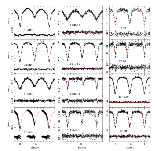
Figure 30: $I-$band light curves with $O-C$ residuals. See text for comments on individual stars.

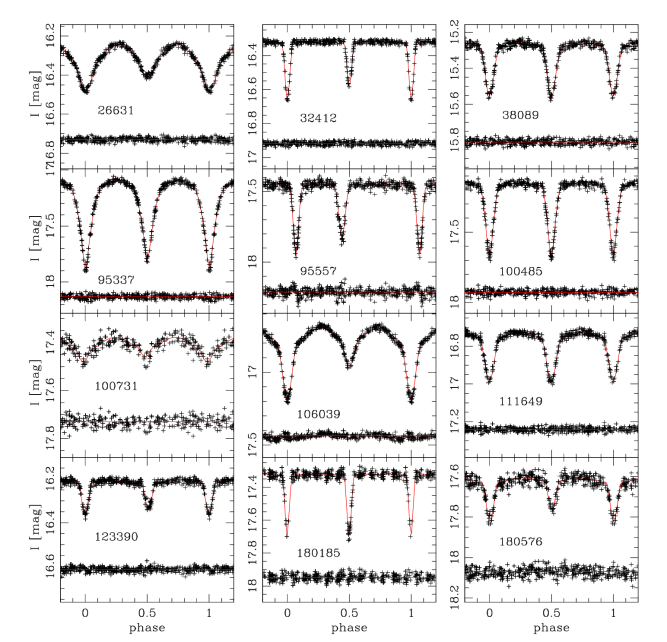
Figure 31: Same as Fig. 30, for 12 more stars.

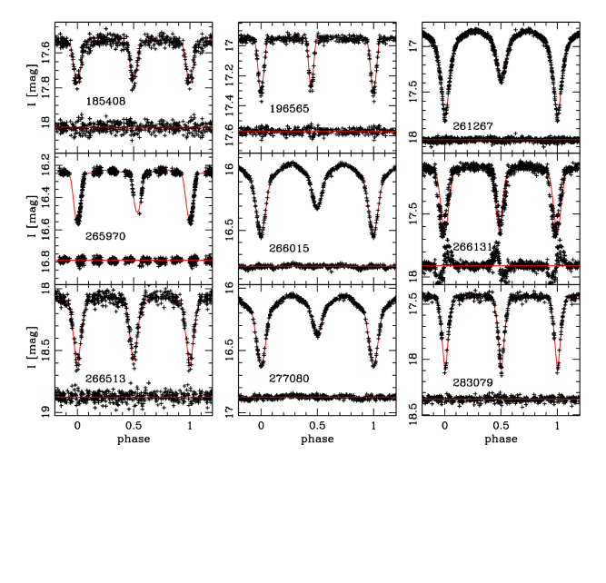
Figure 32: Same as Fig. 30, for nine more stars.

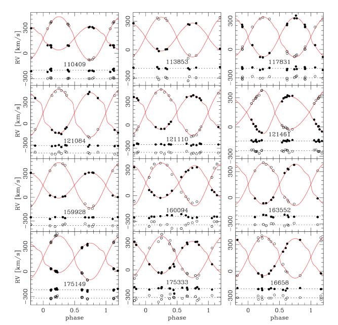
Figure 33: Radial velocity data and best-fitting RV curves.The $O-C$ residuals are shown with a different arbitrary offset for each component. See text for comments on individual stars.

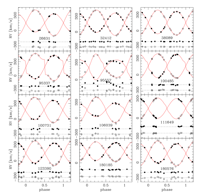
Figure 34: Same as Fig. 33, for 12 more stars.

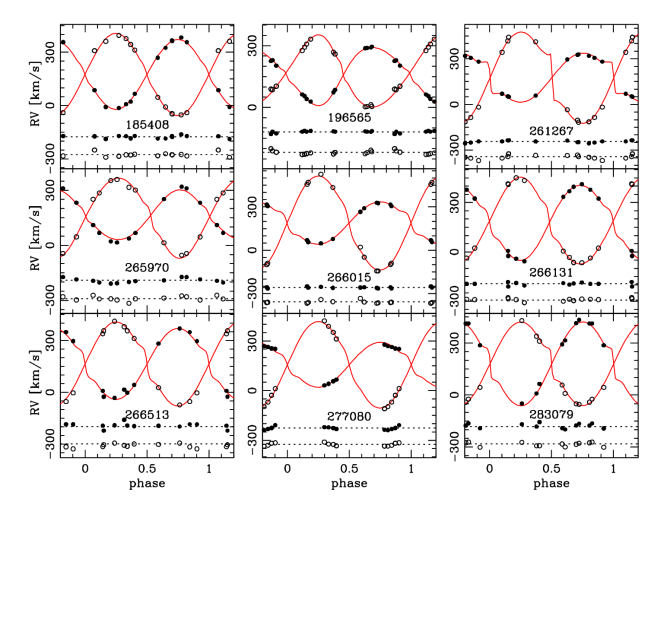
Figure 35: Same as Fig. 33, for nine more stars.

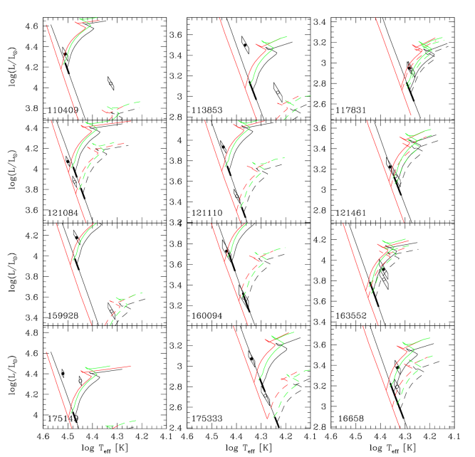
Figure 39: HR diagrams: the positions of the primary and the secondary components are indicated by filled and open symbols, respectively. The primary is the component with the larger mass. The evolutionary tracks from Charbonnel et al. (CMMSS93 (1993)) at $Z=0.004$, corresponding to the observed masses, are indicated by solid (primary) and dashed black lines (secondary). Since these authors adopt a helium content $Y=0.24+3\times\Delta Z$, the helium content of these models is $Y=0.252$. The oblique line corresponds to the ZAMS. The bold segments on the ZAMS, at the departure point of the evolutionary tracks, indicate the $\pm 1\,\sigma$ error on the mass. The red tracks and ZAMS correspond to a poorer metallicity $Z=0.001$ (Schaller et al. SSMM92 (1992)) and a helium content $Y=0.243$. The green tracks are interpolated from the $Z=0.004$ models of Claret & Gimenez (CG98 (1998)) for a helium content $Y=0.28$; thus, they show the effect of a helium enhancement $\Delta Y=0.028$ relative to the tracks of Charbonnel et al. (CMMSS93 (1993)). See text for comments on individual stars.

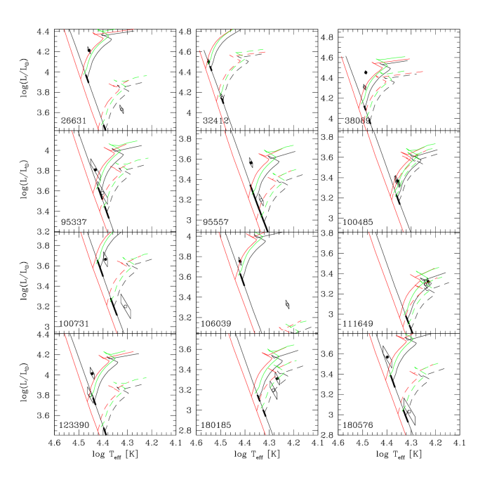
Figure 40: Same as Fig. 39, for 12 more stars.

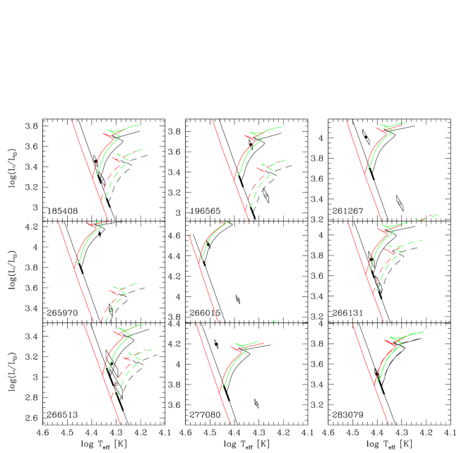
Figure 41: Same as Fig. 39, for nine more stars.

The $I-$band light curves and the best-fit solutions are shown in Figs 30-32. The RV curves are shown in Figs 33-35. The mass-$\log g$ diagrams are shown in Figs 36-38. The HR diagrams are shown in Figs 39-41. The parameters found from the WD/PHOEBE analysis are given in Tables 11 (orbital parameters) and 12 (temperature ratios, potentials and luminosity ratios). The astrophysical parameters of the primary and secondary components are given in Tables 13 and 14, respectively. Finally, the RMS scatters of the light curves and RV curves are summarized in Tables 16 and 17.

4.1 4 110409

With a difference of 0.04 mag in the brightness level between phase 0.25 and phase 0.75, this semi-detached system displays the most asymmetric light curve among all the systems studied in this paper. The light curve is bright ($I^{\mathrm{q}}<16$ mag) and of high quality, with a low RMS scatter combined with a deep primary eclipse ($\Delta I_{\mathrm{minI}}/\sigma_{I}$ $\sim$ 65). This EB-type light curve shows a relatively strong depression occurring just before the primary minimum. Actually, this is strong evidence for absorption by a gas stream stemming from the (inner) L1 Lagrangian point and seen in projection against the primary surface (HHH05). As a consequence, the use of a “simple” symmetric model for the light-curve fit is not satisfactory, resulting in a rather poor fit despite the intrinsic quality of the observations. Therefore, this solution was subsequently improved by adding a cool spot on the equator of the primary component (see Section 3.7). The parameters of the spot are: a colatitude of $\pi/2$ rad (fixed), a longitude of 0.569 rad, an angular radius of 0.3 rad and a temperature factor of 0.6, i.e. the effective temperature of the spot is $0.6$ that of the rest of the stellar surface. Although this new synthetic light curve gives a far more satisfactory fit, the $O-C$ curve reveals that this system is certainly more complex than this “one circular cool spot” model. Actually, there are still some discrepancies at the bottom of the eclipses and just after the secondary minimum. Nevertheless, this model is certainly sufficient to set reliably the inclination, the brightness ratio of the components and the maximum out-of-eclipse flux. On the finding chart, the image of this star is slightly elongated in the EW direction, suggesting a blend with another, fainter star which would lie $1\arcsec$ or slightly farther away to the West. Nevertheless, no clear sign of a 3rd light is seen in the lightcurve.

The RV curves are well constrained with 11 out-of-eclipse spectra and notably observations close to phase 0.75. This system was previously studied by HHH05. There is significant differences between their RV parameters and ours. Our RV semi-amplitudes are 135 and 259 km s^-1, to be compared to their values of 160 and 247 km s^-1. Beside having lower $S/N$ and resolving power than us, in this particular case the discrepancy is certainly due to their admitted lack of observations close to the quadratures. Consequently, our value for the mass ratio, $q=0.52$, is certainly more secure than theirs (0.65).

We found a spectroscopic $B$ luminosity ratio of 1.45. This is higher than the photometric value (1.29), perhaps because of the large distortion of the Roche lobe filling companion. Interestingly, the brighter, i.e. primary, component has lower monochromatic luminosities than the secondary component: even though the primary has a higher bolometric luminosity, it emits mostly in the UV part of the spectrum, so that its $I$ luminosity, for instance, is lower than for the secondary.

The most interesting parts of the disentangled spectra of both components are presented in Fig. 4. As a consequence of the low $B$ luminosity of the primary, the spectrum of the latter is the noisier of the pair. Not surprisingly, in both spectra the most prominent features are the H i and He i lines. It is tempting to identify a number of features in the primary spectrum with the C ii 4267, O ii 4276-4277, Si iii 4553, Si iv 4089 and Si iv 4116 lines. Nevertheless, both the lack of positive identification of the He ii 4542 line for a $\sim$14 $\mathcal{M}_{\odot}$ star and the noisy profile of the He i lines mean that one must be careful in not over-interpreting a spectrum of rather low quality. The better secondary spectrum displays cleaner features. The He i 4471 and Mg ii 4481 lines allow to secure the temperature of the secondary.

By fixing the photometric temperature and $B$ luminosity ratios, a least-squares fit of the 11 out-of-eclipse spectra provided a primary temperature very close to $32\,500$ K, that is to say 7000 K more than what was determined by HHH05.

Both mass-$\log g$ and the HR diagrams are typical of a massive Algol-type binary. The brighter and more massive component of the system appears to be close to the zero-age main sequence (ZAMS), while the secondary component is larger and far more luminous than a non-evolved star of the same mass.

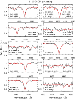
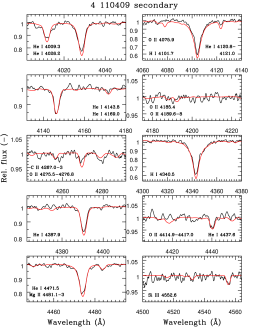
Figure 4: Sections of the disentangled spectra of the primary and secondary components of the binary 4 110409. The scale on the vertical axis is adapted to the size of the features in each section. The red line represents the best fit synthetic spectrum shifted to the systemic velocity. Beside prominent H i and He i lines, Mg ii and Si iii lines are visible in the spectrum of the secondary. The spectrum of the primary is far less convincing; nevertheless Si iv lines seem to be present next to H$\delta$.

4.2 4 113853

The best fit was obtained with a semi-detached model. Because of a moderate RMS scatter (0.017) combined with shallow eclipses ($\sim$0.18 mag) if not purely ellipsoidal variations, the light curve of this binary is one of the poorest of the whole sample. This low amplitude is due to a low inclination ($\sim$60$\degr$). The $O-C$ curve reveals that the profiles of the eclipses are not perfectly symmetrical. The quality of the data is not sufficient, though, to trace the possible astrophysical cause of this asymmetry. On the finding chart, the star seems fairly well isolated.

Despite only 7 out-of-eclipse spectra, the RV curves are rather well constrained with observations close to both quadratures.

The $S/N$ of the composite spectra are low ($25-65$) and there is a sizeable nebular emission in the Balmer lines. Because of the lack of metallic lines and the severe contamination of the Balmer lines by nebular emission which hinder the disentangling procedure, the disentangled spectra of the components were not used. The least-squares fit was performed, letting both temperatures and the $B$ luminosity ratio free to converge. It provided a temperature ratio remarkably close to the photometric one, and a spectroscopic $B$ luminosity ratio of $0.68$, also in perfect agreement with the photometric ratio ($0.68$). Thus, fixing the temperature and luminosity ratios to the photometric values was not needed to determine a reliable temperature of the primary.

Both the mass-$\log g$ and the HR diagrams show an evolved system with a primary component seemingly half-way between the ZAMS and the terminal-age main sequence (TAMS). On the HR diagram, the primary lies much higher than the evolutionary track corresponding to its mass. Whether this is due to a temperature overestimate (linked e.g. with an underestimated sky background) or to some evolutionary effect remains to be examined. Besides, the distance modulus perfectly agrees with the currently accepted value for the SMC.

4.3 4 117831

This faint system has a low-to-medium quality light curve of the EA type. There is a slight ellipsoidal variation between the eclipses and the latter have a similar depth ($\sim$0.4 mag). This is a close detached system with similar components. The finding chart suggests a possible slight blend with a fainter star located some $1\arcsec$ to the East of the system. No clear sign of a 3rd light, however, is seen in the lightcurves.

The RV curves are well constrained with 12 out-of-eclipse spectra and observations close to phase 0.25 and phase 0.75. The mass ratio close to one ($q=0.98$) is indicative of a binary with ‘twin’ components.

The disentangled spectra are of too low quality to see any useful metallic line. The Mg ii 4481 and C ii 4267 are barely visible. Disentangling of the Balmer lines was hindered by the strong emission. A first least-squares fit provided both temperatures and a poorly constrained spectroscopic $B$ luminosity ratio of $0.97\pm 0.11$. The WD code converged to a higher luminosity ratio ($1.17\pm 0.05$), even when we tried to minimize it by fixing the potential of the primary. The temperature of the primary was finally set by a fit where the ratio of temperatures was fixed to the photometric value, and the luminosity ratio assumed equal to one. The small number of photometric data in the minima, especially the primary one, probably makes the photometric luminosity ratio unreliable and explains why the radius of the primary component appears slightly smaller than that of the secondary one.

According to the mass-$\log g$ diagram, the age of the system is about $50$ Myr, assuming the standard SMC metallicity $Z=0.004$. The positions of both components in the HR diagram agree to within the error bars with the evolutionary tracks.

This system was studied by Wyithe et al. WW02 (2002) (see Table 6). Their results not being constrained by spectroscopy, it is not surprising that they found a very different solution. They considered this system as a semi-detached binary with a photometric mass ratio of 0.157. Our spectroscopic results completely rule out that model.

4.4 4 121084

This system displays deep eclipses ($>0.6$ mag) of similar depth. A slight ellipsoidal variation is visible. This is clearly a close detached system with slightly distorted twin components. No clear sign of crowding is seen on the finding chart, except possibly with very faint neighbour stars.

The RV curves are well constrained with 9 out-of-eclipse observations regularly distributed around the quadratures.

The composite spectra are polluted by strong nebular emission in both H$\gamma$ and H$\delta$ lines. Nevertheless, the widely separated Balmer lines allow a reliable temperature and luminosity ratio determination. The disentangled spectra are useful to confirm the rather high $V_{\mathrm{rot}}\sin i$ values of the components. Not surprisingly, no metallic lines are visible because of the moderate $S/N$ combined with fast rotational velocities. The potential of the primary was fixed so that the luminosity ratio given by the WD code matches the spectroscopic one. The temperature of the primary was obtained by fixing the temperature ratio to the photometric one,

Both stars lie on the ZAMS, both in the mass-$\log g$ and HR diagrams. On the HR diagram, however, they are clearly more luminous and hotter than their expected positions for a metallicity $Z=0.004$. They would better agree with the ZAMS and evolutionary tracks for $Z=0.001$, as many other systems do. Moving the representative points to the their expected positions for $Z=0.004$ would require a $2000$ K decrease in effective temperature; that seems large, but the residuals between the observed and synthetic composite spectra show only very subtle changes. Only a modest systematic effect might be responsible.

4.5 4 121110

The medium-to-high quality light curve shows a deep ($\sim$0.5 mag) primary eclipse. A slight ellipsoidal variation is visible between the eclipses. This is again a close detached system with slightly distorted components. No star closer than $3\arcsec$ is seen on the finding chart, except for a very faint one lying about $2\arcsec$ away to the SW.

The RV curves are well constrained with 11 out-of-eclipse spectra.

There is strong nebular emission in both Balmer lines. The spectroscopic $B$ luminosity ratio ($0.415\pm 0.047$) nicely agrees with the photometric one (0.424), without any need for fixing the potential of the primary. The temperature of the primary was fitted after fixing the temperature and luminosity ratios to their photometric values, as ususal. The Si iii 4553 line is clearly visible on the disentangled spectrum of the primary. The lack of Mg ii 4471 confirms the relatively high temperature of the primary. The spectrum of the secondary is too noisy for the identification of metallic lines.

On the mass-$\log g$ diagram, the stars match an isochrone corresponding to about $7-8$ Myr. In the HR diagram, the positions of both components are above the $Z=0.004$ evolutionary tracks but are consistent with the lower metallicity ones ($Z=0.001$). Increasing the helium content would also help to reconcile their positions with the evolutionary tracks, unless a systematic effect raises the apparent effective temperatures.

4.6 4 121461

This is an eccentric system with two (relatively) widely separated components. Both eclipses are very similar in depth and width. With $I^{\mathrm{q}}\sim 17.9$ mag, this is one of the faintest systems in our sample. Nevertheless, the finding chart indicates no crowding problem whatsoever. No significant apsidal motion was found on the basis of photometry. An analysis with the EBOP code shows that the $\omega_{0}$ value depends critically on the $e\sin\omega_{0}$ quantity, which is poorly constrained, while the more robust $e\cos\omega_{0}$ quantity is such that $\cos\omega_{0}\simeq 0.75$ and thus does not constrain $\omega_{0}$ very tightly. Fig. 5 suggests a marginal decrease of $e\cos\omega_{0}$ with time which, if real, could only be due to gravitational perturbations from a third body, because $\dot{\omega}<0$, while pure tidal effects always result in $\dot{\omega}>0$. We have assumed no apsidal motion.

Figure 5: Variation with time of the $e\cos\omega$ quantity of the system 4 121461, determined with the EBOP code on the basis of the $I$ magnitudes grouped in four time intervals. The solid line corresponds to a hardly significant negative apsidal motion, while the dashed horizontal line indicates no apsidal motion, for $e=0.185$ and $\omega_{0}=222.8^{\circ}$.

This system is one of the two in our sample having 16 out-of-eclipse spectra, of which 15 were used (the 8th one has too poor SNR). There is a sufficient number of observations close to the quadratures.

The composite spectra are very noisy. The disentangled spectra are of very low quality, with no exploitable metallic lines. There is strong nebular emission. Letting the temperature of both components free to converge (together with the $B$ luminosity ratio) resulted in very uncertain values, so we fixed the temperature ratio to the photometric one in order to estimate the temperature of the primary. The rotational velocities were fixed to the pseudosynchronized values. A luminosity ratio of $0.95\pm 0.06$ was found on the basis of the spectra, which agrees well with the photometric one ($0.91\pm 0.03$) obtained without fixing the potential of the primary. The photometric luminosity ratio was adopted, which results in almost identical radii for the components. This results in a slightly lower surface gravity on the secondary component than on the primary, because of the mass ratio, but this difference is not significant.

On the mass-$\log g$ diagram, this system lies close to the ZAMS but might be up to $15-20$ Myr old. The positions of the stars in the HR diagram agree, within the error bars, with the evolutionary tracks, although they tend to lie too high, as is the case of other systems.

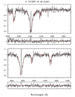
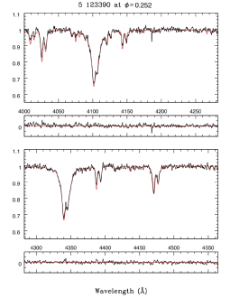
Figure 6: Example of observed spectra close to a quadrature. Both spectra are at the same scale. The red line represents the composite synthetic spectrum of the binary system, i.e. the addition of the scaled and velocity-shifted synthetic spectra of the two components for the corresponding orbital phase. Beside a low $S/N$, the spectrum of 4 121461 shows strong nebular emission in the Balmer lines. From the best fit, the $B$ luminosity ratio was found to be $\sim$0.95 with a primary temperature of $\sim$22 000 K. The spectrum of 5 123390 points to a $B$ luminosity ratio of 0.59 and a primary temperature of 27 000 K.

4.7 4 159928

This system presents low-to-medium quality light curves of the EW type with eclipses of unequal depth. The RMS scatter of the light curve is rather low, but the minima are not very deep ($\Delta I_{\mathrm{minI}}\sim 0.25$ mag). It can be inferred from this that the system comprises close, strongly distorted components of unequal brightness. The best-fitting model corresponds to a semi-detached binary with a low inclination, close to $60\degr$. The finding chart shows a well isolated target, except for a quite faint neighbour at about $2\arcsec$ to the NNE.

There are only 8 out-of-eclipse spectra, but they are close to the two quadratures.

A spectroscopic luminosity ratio of 0.45 was found in the $B$ band, which is higher than the photometric value (0.36). The temperature of the primary was determined by fixing the temperature and luminosity ratios to the photometric values, after suppression of the very strong nebular emission lines. The Si iii 4553 line is the only metallic line clearly visible in the disentangled spectrum of the primary. The spectrum of the secondary shows no exploitable metallic line. The Mg ii 4481 is barely visible. The synchronized values for $V_{\mathrm{rot}}\,\sin i$ are close to 200 km s^-1 and therefore all but the strongest lines are buried in the noise.

Both the mass-$\log g$ and HR diagrams show positions typical of a semi-detached system with an evolved secondary component. The primary is slightly overluminous relative to the evolutionary track of a single star.

4.8 4 160094

This detached system of moderate eccentricity presents low-to-medium quality light curves with rather shallow eclipses ($\Delta I_{\mathrm{minI}}\sim 0.20$ mag). Except for a few very faint neighbours, the target seems free from crowding on the finding chart.

There are 11 out-of-eclipse spectra. Both quadratures are well covered by the observations.

The $T_{\mathrm{eff}}$ of the primary was determined together with that of the secondary and with the $B$ luminosity ratio. The temperature of the secondary proved rather ill-defined, so the photometric temperature ratio was used to define it, as usual. The potential of the primary was fixed to a value that implies a luminosity ratio close to the spectroscopic one. No metallic lines are visible in the very noisy disentangled spectra. The nebular emission is strong in both H i lines.

Despite the moderate quality of the photometric and spectroscopic data, the positions of both stars fall right on the ZAMS in the mass-$\log g$ diagram. In the HR diagram, their position agree well with the evolutionary tracks, though they appear slightly overluminous.

A notable characteristic of this system is its fast apsidal motion $\dot{\omega}=9.8\pm 1.9$ $\degr$ yr^-1. Figure 7 shows the $e\cos\omega$ product as a function of time, as obtained using the EBOP code. The solid line represents the WD solution, which appears consistent with the EBOP results, even though the latter would be compatible with a faster apsidal motion coupled with a slighly smaller eccentricity. Further discussion of this result is deferred to Section 5.

Figure 7: Variation with time of the $e\cos\omega$ quantity of the 4 160094 system, determined with the EBOP code on the basis of the $I$ magnitudes grouped in four time intervals. The solid line corresponds to the parameters listed in Table 11.

4.9 4 163552

This is one of the five systems with $I^{\mathrm{q}}<16$ mag, displaying a high quality light curve of the EB type. The eclipses have very similar depths ($\sim 0.4$ mag), indicating that the temperature ratio is very close to unity. Some faint neighbours are seen on the finding chart about $2\arcsec$ from the target, and it is difficult to judge whether closer neighbours might lurk within the relatively large spot left by this bright system. According to the light curve, there is a substantial third-light contribution to this system: we find $\ell_{3,I}\sim 0.12$, while Graczyk (dG03 (2003), hereafter dG03) found $\ell_{3,I}\sim 0.26$. A significant ellipsoidal variation is indicative of tidally distorted components, though the system is still in a detached configuration.

There are only 9 out-of-eclipse spectra, but the RV curves are well constrained near quadratures.

The observed spectra of this binary were roughly corrected for the presence of a third component, by subtracting a constant from the normalized spectra. The value of the constant was adjusted until the effective temperatures obtained from the least-squares fit to the corrected spectra give a reasonable match to the evolutionary tracks at the metallicity $Z=0.004$ in the HR diagram. A constant of 0.1 only proved sufficient to this purpose, which is widely different from dG03’s photometric estimate of the third light, $\ell_{3,B}\simeq 0.26$. On the other hand, our WD analysis resulted in $\ell_{3,B}\simeq 0.14$, which is more consistent with our rough spectroscopic estimate. Actually, a first attempt to analyze this system resulted in highly overluminous components. This was interpreted as a clear sign that the observed spectra were severely contaminated by the object responsible for the photometric third light.

The disentangled spectrum of the primary shows a faint Mg ii 4481 line and a noisy Si iii 4553 line. These lines were used to constrain the temperature of the primary. The Si iii 4553 line is visible in the spectrum of the secondary too.

This system was studied by HHH05, dG03 (see his Fig. 6) and WW02. Only dG03 took the third-light contribution into account. Not surprisingly, our photometric solution is very close to theirs.

Since we adjusted the amount of third light so that the primary component have a realistic luminosity, the HR diagram shows a primary close to the stellar evolutionary track of a 9.6 $\mathcal{M}_{\odot}$ star, and a secondary close to the evolutionary track of a 9.1 $\mathcal{M}_{\odot}$ star. Their positions are clearly far from the zero-age main sequence. From the mass-$\log g$ diagram, the age of the system is estimated to be 20 Myr. As the position of the primary was inferred from the expected position in the HR diagram, the proposed solution is not entirely reliable and thus is not used for the determination of the mean distance modulus of the SMC (see Section 5.6).

4.10 4 175149

The medium-to-high quality light curve of this system is of the EB type; unfortunately, most of the right part of each eclipse is missing. That is due to a period very close to $2$ days exactly. The minima are fairly deep ($\Delta I_{\mathrm{minI}}\sim 0.50$ mag), well-defined and of unequal depth. There is a strong ellipsoidal variation. The binary is a semi-detached system, with distorted components of different brightnesses. A slight depression occurring before the primary eclipse is indicative of a gas stream. However, we did not venture into adding a spot on the primary in order to mimick this effect, because we felt that the large gaps in the light curve already limit the reliability of the proposed solution.

This system is close to the edge of the CCD used in the OGLE II survey, so it was also listed under the designation 5 38079 in the OGLE database. Thanks to that circumstance, there are 574 photometric $I$ magnitudes instead of less than 300. An examination of the OGLE finding chart reveals that this binary is clearly blended.

This is the second system with 16 out-of-eclipse spectroscopic observations. Because of the 2-day period, all these observations took place before the quadratures. Nevertheless, the RV curves seem to be sufficiently constrained.

A spectroscopic $B$ luminosity ratio of 1.39 was found, though with a large scatter ($\sigma\sim 0.14$). This is higher than the photometric value (1.18). The disentangled spectra are fairly good. The spectrum of the hot primary component displays the He ii 4200 and 4542 lines. The Si iii 4553 and a faint Si iv 4089 lines are equally visible. These lines provide strong constraints for the temperature of the primary. The best-fitting primary temperature was obtained after fixing the temperature and luminosity ratios to the photometric values.

The mass-$\log g$ diagram shows the typical oblique orientation of the segment connecting the components of an evolved binary. The HR diagram shows a highly overluminous primary, relative to the evolutionary track of a 11.8 $\mathcal{M}_{\odot}$ star, and an evolved secondary far more luminous than a main-sequence star of 7.8 $\mathcal{M}_{\odot}$. One may wonder, whether the strange position of the primary is due to an unrecognized third light, both in photometry and spectroscopy, or to some evolutionary effect. In any case, there is no obvious third light in the light curve.

4.11 4 175333

This slightly eccentric system presents low-to-medium quality light curves of the EA type. This is one of the few systems with $I^{q}>17.5$ mag. Consequently, the $O-C$ curve shows a relatively high scatter. The minima are of unequal depth. A slight ellipsoidal variation is visible. This is clearly a detached system with components of unequal brightness. The target appears perfectly isolated on the finding chart.

There are 14 out-of-eclipse spectra. The observations constrain well the RV curves.

This system was studied by WW01. The fact that they consider the eclipses as total (while we consider them as partial) and their lack of spectroscopic constraints on their ratio of radii account for the differences between their solution and ours. The evidence for total eclipses does not appear compelling, so additional photometry would be needed to settle the issue. We found a spectroscopic $B$ luminosity ratio of 0.55, slightly smaller than that finally adopted taken photometry into account. The disentangled spectrum of the primary shows a noisy Mg ii 4481 line. The spectrum of the secondary is too noisy to detect any metallic line. The temperature of the primary was fitted with the temperature and luminosity ratios fixed to the photometric values. The fit with both temperatures free to converge, together with the luminosity ratio, gave a rather large scatter of about $1600$ K and a secondary temperature about 900 K cooler. In spite of the partial eclipses, there was no need to fix the potential of the primary in order to find a $B$ luminosity ratio that matches the spectroscopic value, so the photometric value of the luminosity ratio was adopted.

On the mass-$\log g$ diagram, both stars fall right on the 20 Myr isochrone. On the HR diagram, however, both stars appear significantly overluminous relative to their evolutionary tracks, suggesting that the effective temperatures may be overestimated by at least $2000$ K! Strangely enough, the colour excess of this system appears to be small ($E(B-V)=0.07$) and the distance modulus ($18.6$) clearly smaller than the accepted value for the SMC ($\sim 18.9-19.0$). If the effective temperatures had indeed been overestimated, this would have implied both a too blue intrinsic colour and a too large intrinsic luminosity (hence a more negative absolute magnitude), se one would rather expect a large colour excess and a large distance modulus.

4.12 5 016658

This close detached system presents medium quality light curves with eclipses of equal depths, and is composed of tidally distorted twin components. The finding charts reveals no crowding problem.

There are 11 out-of-eclipse spectra. The RV curves are well constrained by the observations around phase 0.25.

This system was studied by WW01. As for the previous binary, the differences observed between their (photometric) solution and ours is due to their lack of a spectroscopic constraint on the ratio of radii, and to the fact that they assume total eclipses. Evidence for the latter is not compelling, however, and awaits further photometric measurements for confirmation. A spectroscopic $B$ luminosity ratio of $\sim$0.60 was found, which guided the choice of the potential of the primary component in the WD analysis. The Mg ii 4481 line is clearly visible on the disentangled spectrum of the primary. The spectrum of the secondary is too noisy to show any metallic line. The best-fitting primary temperature was obtained simultaneously with the temperature of the secondary, which appeared quite compatible (within $300$ K) with the photometric one (i.e. given the spectroscopic primary temperature and the photometric temperature ratio), and with the luminosity ratio. The photometric temperature ratio was adopted.

On the mass-$\log g$ diagrams, both stars fall on the 30 Myr isochrone within the errors. On the HR diagram, the primary has a position compatible with its evolutionary track within errors, though it appears slightly too luminous. The secondary is slightly hotter than the primary, and is more overluminous; still, it remains compatible with its evolutionary track if the errors on both luminosity and mass are considered.

4.13 5 026631

This system presents a medium-quality light curve of the EW type with minima of unequal depth. This is clearly a semi-detached system with strongly distorted components of unequal brightness. It presents the second lowest inclination of the sample with $i\approx 61\degr$, implied by the rather small amplitude of the light curve. No blend is apparent on the finding chart, except for two or three very faint neighbours at about $2\arcsec$.

There are only 8 out-of-eclipse spectra, but these ones are sufficiently constraining to get reliable RV curves.

A spectroscopic $B$ luminosity ratio of 0.74 was found, while the photometric value is 0.50. The disentangled spectra show no useful metallic lines. This is due notably to the high $V_{\mathrm{rot}}\,\sin i$ values ($\sim$190 km s^-1). The temperature of the primary was obtained by fixing the temperature and luminosity ratios to the photometric values.

The mass-$\log g$ and HR diagrams show the typical positions for the components of a semi-detached system, with the primary near its expected evolutionary track and an overluminous secondary. The primary is slightly overluminous relative to its track, as is often the case in this work, while the secondary is slightly below its track, a rare occurrence.

This binary was studied by HHH05. Their primary temperature ($25\,500$ K) and mass ratio ($\sim$1) differ noticeably from our values.

4.14 5 032412

This wide, detached system presents medium-to-high quality light curves with minima of unequal depth, betraying components of unequal brightness. The target appears well isolated on the finding chart.

There are 13 out-of-eclipse spectra. The RV curves are very well constrained and the RMS scatters are low. Interestingly, both the light and velocity curves indicate a negligible eccentricity, in spite of the small relative radii of the components, as if circularization had taken place during the protostellar phase. Note that this is the most massive system of our whole sample: its total mass reaches $30\leavevmode\nobreak\ \mathcal{M}_{\odot}$.

A spectroscopic $B$ luminosity ratio of 0.55 was found. The disentangled spectra are of high quality (Fig. 8), even for the H i lines. Beside the H i and He i lines, the following lines are visible in the spectrum of the primary: He ii 4200 and 4542 (strong), Si iv 4089, Si iv 4116, O ii 4185, Si iv 4212, O ii 4276-7 and Si iii 4553. An effective temperature of about 35 000 K was inferred from the best-fitting synthetic spectrum.

The following metallic lines are visible in the disentangled spectrum of the secondary: Si iv 4089, Si iv 4116, O ii 4185, O ii 4190, C ii 4267, O ii 4276-7, O ii 4415-7, Mg ii 4481 and Si iii 4553. He ii 4542 is clearly visible too. Comparing the relative depths of Mg ii 4481 with He i 4472, He ii 4542 with Si iii 4553, C ii 4267 with O ii 4276-7, Si iv 4089 and Si iv 4116 with He i 4121 allows to estimate an effective temperature close to 31 000 K. Thanks to the good SNR of the spectra, fitting simultaneously the temperatures of the components and the luminosity ratio resulted in a temperature ratio very close to the photometric one. Nevertheless, the adopted temperatures are those obtained by imposing the photometric ratio.

The mass-$\log g$ diagram shows a very young binary with both components on the ZAMS. On the HR diagram, the positions of both components agree fairly well with the stellar evolutionary tracks of 17.1 and 13.1 $\mathcal{M}_{\odot}$ stars. However, the primary appears slightly overluminous relative to its track.

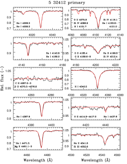
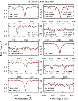
Figure 8: Sections of the disentangled spectra of the primary and secondary components of the binary 5 032412. The scale on the vertical axis is adapted to the size of the features in each section. The red line represents a velocity-shifted synthetic spectrum of the star. Beside prominent H i and He i lines, He ii, O ii, Mg ii, Si iii and Si iv lines are visible in both spectra. The strong He ii 4542, next to a smaller Si iii 4553 line, and the He ii 4200 line confirm the high temperature of the primary ($\sim$34 900 K). The lower temperature of the secondary is confirmed by the stronger Mg ii 4481 line and the smaller He ii lines.

4.15 5 038089

This bright detached system presents medium-quality light curves with eclipses of very similar depth. Therefore, the components are very similar.

This system has abnormal colour indices (see Table 3 and Fig. 3), which suggests the presence of a third light. An examination of the OGLE finding chart reveals that this binary is clearly blended, though with much fainter stars.

There are 11 out-of-eclipse spectra. The RV curves are very well constrained and the RMS scatter is remarkably low.

A spectroscopic $B$ luminosity ratio of 0.68 was found. The eclipses are not very deep, so we fixed the potential of the primary to reproduce this luminosity ratio. The disentangled spectra, shown in Fig. 9, are very similar. Strong He ii 4200 and 4552 lines are visible in both spectra. The following metallic lines are equally identifiable (Fig. 9): O ii 4076, Si iv 4089, Si iv 4116, O ii 4185, O ii 4190, C ii 4267, O ii 4276,O ii 4415-4417, Si iii 4553. This wealth of lines allows to determine the temperatures of both components with a great accuracy. From the best-fitting synthetic spectra, we found 30 400 K and 30 800 K for the effective temperature of the primary and secondary, respectively. This is very close (i.e. within $200$ K) to the temperatures estimated from the composite spectra by imposing the photometric temperature and luminosity ratios; thus, one can safely conclude from this example that the two methods are equivalent.

The high quality of the spectroscopic observations allowed to estimate the astrophysical parameters with a greater accuracy than most systems in our sample. On the mass-$\log g$ diagram, both components lie just above the 10 Myr isochrone; their respective positions suggest that the ratio of radii may be slightly underestimated. The HR diagram shows that both stars are significantly overluminous with respect to the evolutionary tracks of 13.0 and 11.7 $\mathcal{M}_{\odot}$ stars. Invoking the blending of the binary with a third-light contributor does not seem to help much. No clear sign of a third light can be seen in the lightcurve; this is admittedly a weak argument, since the light curve of a detached system with weak proximity effects cannot constrain well a third light. But, in addition, a third light will not change much the relative radii of the components, and the effective temperatures seem well constrained by the relative intensities of several lines, so that the luminosities should remain unaffected. Furthermore, the radial velocity curves are of such quality that it is difficult to imagine how the masses could be biased otherwise than through the inclination angle $i$. A third light would make the photometric minima less deep and so, it would mimick a lower $i$. Since the RV amplitudes give the product $\mathcal{M}\sin^{3}i$, underestimating $i$ is equivalent to overestimating $\mathcal{M}$, while we would need the reverse to explain the HR diagram we see. A test with the EBOP code confirms this qualitative argument: assuming a third light $\ell_{3,I}=0.2$ changes the radius of the primary by $-0.26$% only (keeping the ratio of radii constant), so that the luminosity decreases by half a percent, while the inclination is increased by more than three degrees, lowering the masses by $3.6$%. That would imply evolutionary tracks with a luminosity about 0.05 dex lower (or 11%) in the HR diagram. Finally, the distance modulus of this system is very close to the one expected for the SMC. Therefore, for a third light to be the cause of the inconsistency, it can only be via the RV curves, the amplitude of which should be biased to small values by a stationary third spectrum.

This binary was part of the first release of 10 bright SMC systems by HHH03. Comparing our results with theirs, we see that we have similar estimates for the mass ratio and temperatures of the stars, but markedly different values for the masses and radius of the secondary. A photometric solution was proposed by dG03, who do not recommend it for distance determination because its components do not fall on their mass-luminosity relation.

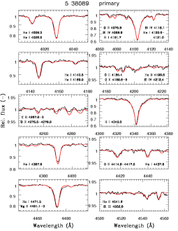
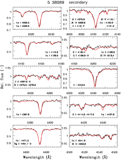
Figure 9: Sections of the disentangled spectra of the primary and secondary components of the binary 5 038089. The scale on the vertical axis is adapted to the size of the features in each section. The red line represents a velocity-shifted synthetic spectrum of the star. Beside prominent H i and He i lines, He ii and a number of fainter metallic lines (C ii, O ii, Si iii, Si iv) are visible. The relative intensities of the He ii 4542 and Si iii 4553 are very useful to constrain the temperature of the two stars.

4.16 5 095337

This is a close but detached system, with tidally distorted components of unequal brightness. The $O-C$ curve suggests that the primary eclipse is not perfectly reproduced by the synthetic light curve, but there is no obvious third-light contribution. The finding chart shows some blends with two or three fainter stars at $1\aas@@fstack{\prime\prime}5$ or so.

There are 10 out-of-eclipse spectra. The RV curves are well constrained with observations close to both quadratures.

A spectroscopic $B$ luminosity ratio of 0.66 was found. The disentangled spectra are of low quality. Because of the low $S/N$ and the high $V_{\mathrm{rot}}\,\sin i$ ($\sim$200 km s^-1), no metallic line can be positively identified. There is some nebular emission in the Balmer lines. The best-fitting synthetic spectra allowed to estimate simultaneously the temperatures of the primary and of the secondary, the ratio of which agrees quite well with the photometric one. In addition, the spectroscopic $B$ luminosity ratio perfectly matches the photometric one, so that the potential of both the primary and the secondary were left free to converge.

On the mass-$\log g$ diagram, both components define a segment which is perfectly parallel and very close to the 10 Myr isochrone. On the HR diagram, however, both components appear strongly overluminous compared to the evolutionary tracks of 8.7 and 7.6 $\mathcal{M}_{\odot}$ stars. Decreasing the effective temperatures by about $1300$ K would reconcile the luminosities with the tracks. However, this looks difficult. The emission in both Balmer lines was suppressed on a 4 Å  range centered on each emission line, and we verified that increasing that range to 8 Å  does not change the estimated temperature in a significant way. Thus, either this system suffers from some bias on the RV curves, or its metallicity is closer to $Z=0.001$ than to $Z=0.004$.

4.17 5 095557

This is the system with the highest eccentricity, displaying a medium quality light curve with minima of unequal depths. The target is perfectly isolated on the finding chart.

There are 11 out-of-eclipse spectra. The RV curves are well constrained with observations close to both quadratures, but the fit is not very good and, unfortunately, most spectra are grouped in the phase interval with the smaller amplitude.

A spectroscopic $B$ luminosity ratio of $\sim$0.5 was found when limiting the fit to the seven spectra for which the radial velocity difference $\Delta RV>250\leavevmode\nobreak\ \mathrm{km\,s^{-1}}$. This ratio increases to 0.63 if all eleven spectra are taken into account, so that this quantity is rather poorly constrained. The disentangled spectra are of very low quality. This is probably due partly to the low $S/N$ of the observed spectra, and partly to some inaccuracies in the orbital parameters. The temperature of the secondary given by the fits to the composite spectra is about $1000$ K higher than the photometric estimate, which was adopted. The pseudosynchronized values of $V_{\mathrm{rot}}\,\sin i$ were adopted.

An apsidal motion is detected at the $5\,\sigma$ significance level, and the WD result is confirmed by the variation of the $e\,\cos\omega$ quantity as given by the EBOP code. The photometric data was divided into four sets and the fits were obtained by fixing the inclination, the ratio of radii and the relative radius of the primary. The result is displayed in Fig. 10 and suggests the apsidal motion to be real. The adopted apsidal motion seems underestimated on that figure, but the constraint imposed by the RV curves has to be kept in mind.

Figure 10: Same as Fig. 7, but for the system 5 95557. The filled black dots represent independent $e\cos\omega$ determinations made on four successive times series containing about the same number of photometric observations in the $I$ band. The solid line is based on the parameters listed in Table 11, while the dotted line corresponds to the fitted $\dot{\omega}+2\sigma$. The horizontal dashed line shows the result obtained from the whole time series under the assumption of a constant $\omega$.

On the mass-$\log g$ diagram, the two components lie right on the 30 Myr isochrone, in spite of the rather large uncertainty on the masses. On the HR diagram, both components appear clearly overluminous relative to their respective evolutionary tracks, as in many other systems.

4.18 5 100485

This is a detached system with ‘twin’ components and a circular orbit. The finding chart reveals no crowding problem, the closest neighbour being at about $2\aas@@fstack{\prime\prime}5$.

There are 13 out-of-eclipse spectra. The RV curves are well constrained, with observations close to both quadratures and small residuals.

A spectroscopic $B$ luminosity ratio of 0.93 was found, which matches the photometric value (0.97) rather well. The disentangled spectra are very similar. The following metallic lines can positively be identified: C ii 4267, Mg ii 4481 and Si iii 4553. These lines allowed to estimate a temperature close to $\sim$22 000 K for each component. The least-squares fit, performed with both temperatures and the luminosity ratio free to converge, provided a temperature ratio very close to the photometric one.

The two components lie right on the 20 Myr isochrone on the mass-$\log g$ diagram, and they are compatible, within the errors, with their respective evolutionary tracks in the HR diagram. Here again, however, they are slightly overluminous, unless their metallicity is low.

4.19 5 100731

This system presents low-to-medium quality light curves of the EW type, with the smallest amplitudes among those in our sample. This is another case of binary seen under an unfavourable inclination ($\sim$60$\degr$). The finding chart shows a perfectly isolated target.

The most satisfying fit of the light curves was obtained with an overcontact model.

There are only 8 out-of-eclipse spectra. Nevertheless, these observations are sufficiently constraining to get reliable RV curves.

Spectroscopy gives a $B$ luminosity ratio of $\sim 0.44$, while the photometric ratio amounts to $\sim 0.51$. As usual, the latter was preferred, especially because of the strong constraints provided by a Roche-lobe-filling pair. The disentangled spectra have a low $S/N$, and a least-squares fit to the composite spectra with both temperatures free provided two temperatures close to $23\,000$ K. However, the scatter of the secondary temperature was high, so the photometric temperature ratio was adopted and fixed.

The mass-$\log g$ diagram shows a secondary component more evolved than the primary, as expected. On the HR diagram, both components appear to be underluminous with respect to their evolutionary tracks, though by a little amount. This is an exceptional occurrence.

4.20 5 106039

This system is a typical semi-detached one. There is a small depression occurring just before the eclipse of the primary, which is strong evidence for a gas stream. We did not attempt to model that stream with a cool spot on the primary, because the distorsion of the light curve remains relatively mild. The target appears perfectly isolated on the finding chart.

There are 9 out-of-eclipse spectra. The RV curves are well constrained with observations close to both quadratures.

A spectroscopic $B$ luminosity ratio of 1.03 was found, in excellent agreement with the photometric value (1.01). The following metallic lines are visible in the disentangled spectrum of the primary: C ii 4267, Mg ii 4481 (faint) and Si iii 4553. A stronger Mg ii 4481 line is equally visible in the spectrum of the secondary. From these lines, the primary temperature was estimated to be close to $25\,500$ K. The least-squares fit, performed with temperature and luminosity ratios fixed to the photometric values, provided a primary temperature $\sim 800$ K higher.

The position of the primary component in the HR diagram is in fair agreement with the theoretical evolutionary track of a 8.6 $\mathcal{M}_{\odot}$ star, though it is slightly overluminous. The evolved secondary component is overluminous with respect to the track of a single star of the same mass.

4.21 5 111649

This is a detached system with very slightly distorted twin components. There is a group of bright stars close to the target on the finding chart, but they are remote enough ($3.5-4\arcsec$) that no 3rd light should be expected from them.

There are 10 out-of-eclipse spectra. The RV curves are not well sampled because the period of 2.95955 days is very close to an integer number of days, but the scatter is small, thanks to the slow projected rotational velocities induced by the relatively long period.

A spectroscopic $B$ luminosity ratio of 0.89 was found, which was imposed (via the potential of the primary) to define the ratio of radii. Indeed, the small amplitude of the light curve prevents a purely photometric ratio to be well constrained. Noisy C ii 4267 and Mg ii 4481 lines are visible in the disentangled spectrum of the secondary. The temperature of the primary was determined from a fit with fixed temperature and luminosity ratios. According to both spectroscopy and photometry, the secondary appears marginally hotter than the primary, the temperature difference being about $2\,\sigma$.

Both components have a very similar mass ($\sim$5.4 $\mathcal{M}_{\odot}$), and according to the mass-$\log g$ diagram, the empirical mass contrast appears a bit too high to match the $\sim 80$ Myr isochrone. Interestingly, both components lie right on the Terminal Age Main Sequence (TAMS), where evolution is so fast that a theoretical lower limit to the mass ratio can be settled. Starting from the purely empirical surface gravities, and increasing their difference by two sigma (so that $\log g_{\mathrm{P}}-1\,\sigma=3.72$ and $\log g_{\mathrm{S}}+1\,\sigma=3.80$), one can read the corresponding masses along the $\log t=7.9$ isochrone. Assuming that both stars have not yet passed the “hook” that marks the end of the mains sequence, the resulting mass ratio is $q=0.98$. But it is quite possible that the primary has just passed the hook while the secondary has not, in which case $q=0.966$. In both cases, the mass ratio is closer to one than the value directly obtained from the RV curves by $0.03$ to $0.04$. Therefore, this system can be considered as hosting real twins.

The position of the primary in the HR diagram agrees almost perfectly with the theoretical evolutionary track, especially if the star has just evolved beyond the “hook”. That of the secondary, however, is a bit too high, as if its mass was underestimated.

4.22 5 123390

This slightly eccentric system ($e=0.042$) presents low-to-medium quality light curves with a small amplitude. This is clearly a detached system with components of unequal brightness. The finding chart shows a neighbour at about $1\aas@@fstack{\prime\prime}5$ to the SW of the binary, which might have polluted the spectra slightly.

There are 14 out-of-eclipse spectra. The RV curves have a small RMS scatter and are very well constrained by the observations.

A spectroscopic $B$ luminosity ratio of 0.58 was found. The disentangled spectra are of fairly good quality. The following metallic lines are visible in both spectra: O ii 4076, C ii 4267, O ii 4276, O ii 4415-4417, Mg ii 4481 and Si iii 4553. For the primary, the best-fitting temperature for these lines is $\sim$26 000 K. The least-squares fit of the composite spectra gave temperatures of $28400$ and $26260$ K for the primary and secondary respectively, but with a large scatter. A plot of the fitted temperatures versus the unnormalized chi-square shows that in some cases, the fit switched components, i.e. attributed the high temperature to the secondary and vice-versa, which partly explains the large scatter (see Fig. 11).

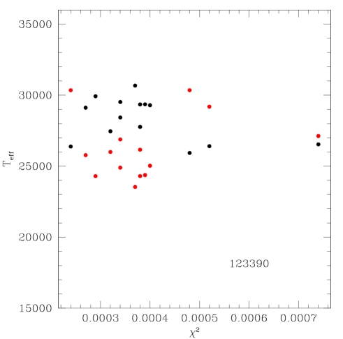
Figure 11: Temperature of the primary (black dots) and of the secondary (red dots) component of the system 5 123390, obtained by fitting composite synthetic spectra to the observed ones, versus the quality of the fit. The trends are roughly horizontal, at least for good fits, which inspires confidence. In a few cases, the components are exchanged (see text).

Strangely enough, the photometric ratio of temperatures is close to one, so that the temperatures become, when fitted while keeping this ratio fixed, $27840$ and $28320$ K for the primary and secondary component respectively. Taken at face value, however, Fig. 11 rather suggests $29000$ and $25000$ K.

According to the mass-$\log g$ diagram, this binary is $\sim$12 Myr old. The position of the primary component in the HR diagram is a bit too high relative to its evolutionary track. The secondary component is much too luminous, falling on the track of the primary! If the purely spectroscopic temperatures were adopted, the primary would be even more overluminous, but the secondary would fall right on its track.

There is a marginally significant apsidal motion of $4.75\pm 1.63$ $\degr$ yr^-1. We show in Fig. 12 the $e\cos\omega$ quantity found with the EBOP code on the basis of the $I$ magnitudes. There is indeed a slight trend corresponding to an increase of $\omega$ with time.

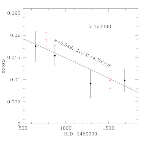
Figure 12: Same as Fig. 7, but for the system 5 123390. The filled black dots represent independent $e\cos\omega$ determinations made on four successive times series containing about the same number of photometric observations in the $I$ band. The open red dots refer to $e\cos\omega$ determinations based on only two time series, but which are twice longer. The solid line is based on the parameters listed in Table 11.

4.23 5 180185

The EA-type light curves of this system are irregularly sampled, because the period is close to $5.5$ days, and there are only very few data in the primary minimum. This is a typical well-detached system with twin components and a small eccentricity. The finding chart reveals a slightly fainter neighbour about $2\arcsec$ away from the target, i.e. far enough that its influence on the spectra may be considered negligible.

This system has unreliable colour indices (see Table 3 and Fig. 3).

There are 12 out-of-eclipse spectra. The RV curves are excellent and well constrained by the observations, with the smallest residuals seen in our sample. The formal errors on the resulting amplitudes are smaller than one percent, allowing mass estimates to within $2-3$%.

A spectroscopic $B$ luminosity ratio of 0.63 was found, which is close to the value given by the WD analysis and finally adopted (0.71). This is the system with the longest period ($P\sim 5.5$ days) in our sample. The long period is responsible for the low $V_{\mathrm{rot}}\,\sin i$ values ($\sim$40 km s^-1) compatible with synchronous rotation. As a consequence, the disentangled spectra of this binary show rather sharp lines. The following metallic lines are visible in both spectra: C ii 4267, Mg ii 4481 and Si iii 4553. The temperature of the primary was obtained as usual by fixing the temperature and luminosity ratios to the photometric values, in spite of the small number of points in the minima. The secondary has a slightly hotter temperature than the primary.

Both components are fairly well aligned on the 50 Myr isochrone in the mass-$\log g$ diagram, although the primary should be slightly more evolved. On the HR diagram, the secondary falls right on its track, while the luminosity of the primary appears too low. This might be due to an unreliable temperature ratio, because of the small number of photometric points in the minima.

4.24 5 180576

This system presents low quality light curves of the EB type. The depths of both minima are rather low and the RMS scatter is high. This is a detached system with components of unequal brightness and a circular orbit. The finding chart shows a close neighbour, at about $1\aas@@fstack{\prime\prime}5$ to the NNW, which might have distorted the temperature estimate of the binary components.

There are 12 out-of-eclipse spectra. The RVs curves are rather good and well constrained by the observations.

A spectroscopic $B$ luminosity ratio of 0.42 was found. This is close to the value reached by the final WD analysis. The observed composite spectra are very noisy ($25\leq S/N\leq 64$) and are contaminated by nebular emission. The disentangled spectra are of rather poor quality. This is partly due to the low reliability of the continuum placement. The C ii 4267 and Mg ii 4481 lines are visible in the spectrum of the primary. The temperature of the primary, determined from a least-squares fit where the temperature and luminosity ratios were fixed, depends on the quality of the fit, as shown by Fig. 13. We adopted the temperature of the primary corresponding to the best $\chi^{2}$, in view of the roughly linear correlation between $T_{\mathrm{eff}}$ and $\chi^{2}$, but without attempting to extrapolate the relation to $\chi^{2}=0$.

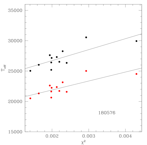
Figure 13: Effective temperatures of the system 5 180576 obtained from a fit to the composite spectra, keeping the temperature and luminosity ratios fixed. Black dots are for the primary, red dots for the secondary. Note that the two curves should be considered as one and the same, since their ratio is constant.

On the mass-$\log g$ diagram, the components are perfectly aligned along the 15 Myr isochrone. The position of the primary component in the HR diagram appears slightly too high relative to the corresponding evolutionary track, while the secondary falls right on its track.

4.25 5 185408

This system presents medium quality light curves of the EA type. The minima are of similar depth and there is some ellipsoidal variation. This is a typical detached system with closely similar components, with medium quality light curves and low amplitude minima of similar depth. The orbit is circular. The $I-$band light curve was cleaned from five outliers before the PHOEBE/WD analysis. The finding chart shows a well isolated target, the closest neighbour being at about $3\arcsec$ to the WNW.

There are 12 out-of-eclipse spectra. The RV curves are excellent, especially in view of the faintness of the object, and well constrained by the observations.

A spectroscopic $B$ luminosity ratio of $\sim$0.64 was found. The WD analysis tended to raise this value and the potential of the primary had to be fixed to keep it close to the spectroscopic one. The C ii 4267, Mg ii 4481 and Si iii 4553 lines are visible in both disentangled spectra. The temperatures were obtained by fixing the temperature and luminosity ratios to the photometric values.

On the mass-$\log g$ diagram, the components are fairly well aligned on the 10 Myr isochrone. On the HR diagram, both components are significantly overluminous with respect to their respective evolutionary tracks, as is often the case.

4.26 5 196565

This detached eccentric system presents medium quality light curves with eclipses of similar depth. The $V$ and $B$ data are missing in the OGLE database. The finding chart shows a neighbour of similar brightness as the target about $2\arcsec$ to the S, raising some concern regarding possible spectral pollution. The results do not confirm these fears, however.

There are 13 out-of-eclipse spectra. The RV curves are very good and well constrained by the observations, in spite of a lack of observations where the expected amplitude reaches its maximum.

A spectroscopic $B$ luminosity ratio of $\sim$0.41 was found, and the potential of the primary was adjusted and fixed in the WD analysis to maintain that value. The C ii 4267 and Mg ii 4481 lines are visible in both disentangled spectra. The least-squares fit of composite synthetic spectra to the observed ones provided a temperature ratio larger than that provided by the photometry, and a primary temperature of $20960\pm 600$ K. Fixing the temperature ratio to the photometric value resulted in the slightly hotter primary temperature that has been adopted.

The mass-$\log g$ diagram suggests that the secondary has a too large radius relative to the primary, as if the luminosity ratio was overestimated: while the primary lies close to the 40 Myr isochrone, the secondary lies on the 50 Myr one. On the HR diagram, however, each component has a position compatible with its respective evolutionary track within the error bars, though the primary is slightly overluminous while the secondary is slightly underluminous.

This system was studied by WW01. Their relative radius of the primary ($0.204$) is very close to ours ($0.200$) but their radius of the secondary ($0.116$) is smaller than ours ($0.150$). The difference is due to the fact that they consider the eclipses as total, while we consider them as partial. Additional accurate photometry in both minima would be welcome to settle the question.

4.27 5 261267

This is a typical semi-detached system with high quality light curves and eclipses of unequal depths. The $O-C$ curve shows no detectable depression before the primary eclipse. Although the finding chart shows a few neighbours, they all lie beyond $2\arcsec$ of the target.

This system has peculiar colour indices (see Table 3 and Fig. 3). Since it lies near the edge of the CCD in the OGLE-II survey, it is also listed under the name 6 11806 in the corresponding database. Thus, there are more than 600 data points in the $I$-band light curve, instead of about 300.

There are 10 out-of-eclipse spectra, which constrain the RV curves relatively well.

Both photometric and spectroscopic ratios are very similar ($\sim$0.4). Because of the relatively high $V_{\mathrm{rot}}\,\sin i$ ($>$150 km s^-1) and moderate $S/N$ of the observations, there are no exploitable metallic lines in the disentangled spectra. The temperature of the primary was obtained, as usual, by least-squares fit to the composite spectra, after fixing the temperature and luminosity ratios to the values given by a preliminary WD analysis.

The mass-$\log g$ and HR diagrams are typical of a massive Algol-type binary. The primary is overluminous relative to the evolutionary track of an isolated star of the same mass, as are other semi-detached systems like 4 113853 and 5 277080.

4.28 5 265970

This slightly eccentric detached system has medium-to-high quality light curves of the EA type. The sampling of the light-curve is incomplete, due to an orbital period close to $3.5$ days. In particular, the depth of the secondary minimum is ill-defined. Therefore, the photometric temperature ratio and inclination are not very reliable. Actually, there is a correlation between these two parameters, in the sense that an increase of inclination implies a decrease of the temperature ratio. The finding chart shows a well defined target, but with an only slightly fainter neighbour about $2\aas@@fstack{\prime\prime}6$ to the NW.

This system lies near the edge of the OGLE-II CCD, and so was measured also on the adjacent chip under the name 6 17345, so that there are as many as 586 data points in the $I$ band. The two data sets were merged after applying a small magnitude offset to each. Using the EBOP code, the fitted magnitude at quadrature and its error was defined for each set, then the mean magnitude at quadrature weighted by the inverse of the variance was computed. Finally, the appropriate offset was applied to each of the two sets to adjust it to this mean magnitude.

There are 10 out-of-eclipse spectra. The RV curves are quite good and well constrained by the observations.

Because of the loose constraints on the light curves, the proposed solution for this system heavily relies on the spectroscopic observations. Nevertheless, the proposed solution meets very well the spectroscopic and photometric constraints, so we consider it as close to reality.

A spectroscopic $B$ luminosity ratio of $\sim$0.23 was found from the usual least-squares fit, which provides the temperature of the primary with an excellent internal precision. The temperature of the secondary is much less certain, because of the small luminosity ratio. In order to maintain the luminosity ratio to the spectroscopic value in the WD analysis, one has to fix the potential of the primary to an appropriate value, and the temperature ratio converges to a smaller value than the spectroscopic one, but still compatible with it given the errors. Thus the photometric temperature ratio was adopted, and the temperature of the primary determined in the usual way.

A number of metallic lines are identifiable in both disentangled spectra: C ii 4267, O ii 4276, O ii 4415-17, Mg ii 4481 and Si iii 4553. There is no emission in the Balmer lines.

The positions of the stars in the mass-$\log g$ diagram are not quite mutually consistent: the ratio of radii should be decreased in order to bring the two components on the same isochrone, which would correspond to about 26 Myr. On the HR diagram, the primary component matches its theoretical evolutionary track surprisingly well, while the secondary has a position consistent with its track within the error bar. The spectroscopic constraints, which are strong, are well fulfilled, but additional photometric data would be useful to improve our solution. This system is especially interesting, because the primary is very close to the TAMS while the secondary is much less evolved.

We applied the EBOP code on four subset of the total time series, after fixing all parameters to their average value, except inclination, $e\cos\omega$, $e\sin\omega$, magnitude at quadrature and phase shift. No significant trend can be seen on Fig. 14, which does not prove, however, that $\omega$ remains constant with time. The less reliable $e\sin\omega$ quantity does not differ significantly from zero according to the EBOP code. In the WD solution, we have arbitrarily imposed a small value $\dot{\omega}=1.8\times 10^{-4}\leavevmode\nobreak\ \mathrm{rad\,day^{-1}}$ which roughly corresponds to the theoretical prediction.

Figure 14: Same as Fig. 7, but for the system 5 265970. The horizontal dashed line shows the weighted average of the $e\cos\omega$ values. The solid line corresponds to $\dot{\omega}\simeq 3.8^{\circ}\,\mathrm{yr^{-1}}$, the expected theoretical value.

4.29 5 266015

This system presents high quality light curves of the EB type with minima of unequal depth. Its bright $I-$band light curve is perfectly well sampled. The small depression occurring just before the primary eclipse is indicative of a semi-detached system with a secondary component filling its Roche lobe and pouring matter onto the primary component. However, the amplitude of this effect was judged too small to justify an attempt to model it through a spot.

There are 10 out-of-eclipse spectra. The RV curves are well constrained by the observations.

A spectroscopic $B$ luminosity ratio of 0.61 was found, rather remote from the photometric value ($0.49$), as is often the case in semi-detached systems. The disentangled spectra of both components have a decent $S/N$ (Fig. 15). Nevertheless, the $V_{\mathrm{rot}}\,\sin i$ being high ($>$150 km s^-1), the small metallic lines are not very conspicuous. The He ii 4120 and 4542 lines are visible in the spectrum of the primary. The Si iii line appears in both spectra. This is one of the few systems with apparently no significant nebular emission lines, therefore the disentangled Balmer lines can be used to find the temperature of the primary. The spectral features of the primary point to a $32\,000$ K star, which is confirmed by the usual least-squares fit.

The positions of the stars in the mass-$\log g$ and HR diagrams are coherent with an evolved system having undergone mass exchange. The primary component is close to the track corresponding to a 15.6 $\mathcal{M}_{\odot}$ star.

This system was studied by WW02. As with most semi-detached systems they studied, their photometric mass ratio proved to be unreliable.

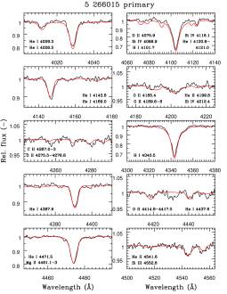
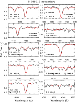
Figure 15: Sections of the disentangled spectra of the primary and secondary components of the binary 5 266015. The scale on the vertical axis is adapted to the size of the features in each section. The red line represents a velocity-shifted synthetic spectrum of the star. Beside prominent H i and He i lines, He ii, O ii, Mg ii, Si iii and Si iv lines are visible in both spectra. The strong He ii 4542, next to a smaller Si iii 4553 line, and the He ii 4200 line confirm the high temperature of the primary ($\sim$32 000 K). Poor continuum placement is responsible for the apparent $O-C$ mismatch of the H$\delta$ line.

4.30 5 266131

The most striking feature of this slightly eccentric detached system ($e\simeq 0.04$) is its huge apsidal motion, which explains the apparently very bad $I-$band $O-C$ curve. An examination of the OGLE finding chart revealed that this binary is slightly blended, but a posteriori, this does not seem to have distorted the results.

This system lying close to the edge of the CCD in the OGLE-II survey, it also exists under the name 6 22883, which doubles the number of data points in the $I$ band. The magnitude at quadrature was determined using the EBOP code for each of the two data sets; the two resulting values agreeing within one thousandth of a magnitude, the two data sets were merged without applying any magnitude offset.

There are 10 out-of-eclipse spectra, which constrain quite well the RV curves.

A spectroscopic $B$ luminosity ratio of $\sim$0.65 was found. As usual with the well detached systems, the potential of the primary was fixed at a value such that this luminosity ratio is preserved through the WD analysis. The $S/N$ of the disentangled spectra are too low to allow any useful metallic line to be seen. Since the temperature ratio is well constrained by the photometric data, the temperature of the primary was determined by fixing this ratio at its photometric value. There is no nebular emission in the Balmer lines.

The mass-$\log g$ diagram suggests that the ratio of radii has been slightly underestimated, since the secondary has a too large surface gravity compared to the primary. Still, the positions of both components are compatible, within the errors, with an isochrone at $7-8$ Myr. The HR diagram shows a good match between the positions of both components and the evolutionary tracks of single 9.0 and 7.7 $\mathcal{M}_{\odot}$ stars. However, both components are slightly overluminous relative to their respective tracks.

The apsidal motion amounts to $\dot{\omega}\simeq 50$ $\degr$ yr^-1, as evidenced by the $e\cos\omega$ values obtained with the EBOP code for four successive subsets of the whole time serie in the $I$ band. That value is confirmed by the WD analysis. The run of $e\cos\omega$ versus time is shown in Fig. 16, together with the best fit curve provided by the WD code. The reality of a very fast apsidal motion is beyond any doubt. It is further discussed in Section 5.

Figure 16: Same as Fig. 7, but for the system 5 266131. The solid line is the best fit provided by the WD code.

4.31 5 266513

This a close detached system with similar components, according to its medium quality light curves with minima of similar depth. The finding charts shows a slightly fainter star at $1.2-1.3\arcsec$ to the W of the target.

There are 10 out-of-eclipse spectra. The RV curves are well constrained by the observations, though the noise is rather large because this system is the faintest in our sample.

A spectroscopic $B$ luminosity ratio of 0.73 was found, but with a large scatter of $0.09$. The potential of the primary was fixed so that the WD analysis preserves a ratio close to that value. The disentangled spectra have a low $S/N$ and no metallic lines are exploitable. Moreover, the Balmer lines are polluted by nebular emission. The photometric temperature ratio is rather well defined, thanks to the large depth of the minima, and was fixed for the determination of the temperature of the primary, as usual for most detached systems.

The mass-$\log g$ diagram shows the two components fairly well aligned along the $\sim 15$ Myr isochrone. On the HR diagram, the primary lies almost exactly on its evolutionary track, while the secondary is slightly overluminous, though its position is quite compatible with the evolutionary tracks within the errors. The luminosity ratio (hence the ratio of radii) seems to have been slightly overestimated.

4.32 5 277080

This system is a typical semi-detached binary with high quality light curves of the EB type. A small depression before the primary eclipse signals the possible presence of a mass-transfer stream. The effect is small enough, however, that we did not deem it worth the effort to model it through a cool spot on the primary.

This system has peculiar colour indices (see Table 3 and Fig. 3). Indeed, an examination of the OGLE finding chart revealed that this binary is strongly blended with a brighter star lying $1\aas@@fstack{\prime\prime}2$ to the SW of the target.

There are 11 out-of-eclipse spectra. Because of an orbital period close to 2 days, there are no observations before the quadratures. In spite of that, the RV curves are rather well constrained. This is one of the few systems showing no nebular emission in the Balmer lines.

A spectroscopic $B$ luminosity ratio of 0.7 was found. This is higher than the photometric ratio (0.57), as seems to be often the case of semi-detached systems. The disentangled spectra are fairly good. A number of metallic lines are visible in the spectrum of the primary: O ii 4185, C ii 4267, O ii 4276-7, Mg ii 4481 and Si iii 4553. The Mg ii 4481 line is the only metallic line detectable in the spectrum of the secondary. The temperature of the primary was determined after fixing the temperature and luminosity ratios to their photometric values.

The positions of the stars in the mass-$\log g$ and HR diagrams are typical of Algol-type system with a secondary more evolved than the primary. The primary component, however, is much more luminous than expected from the evolutionary track of a single star of the same mass, and we cannot guarantee that its effective temperature has not been overestimated. The peculiar HR diagram might be the result of the blend mentioned above with a nearby bright star.

4.33 5 283079

This is a typical detached system with twin components and a circular orbit. The target appears just isolated on the finding chart, with a companion of similar brightness about $2\aas@@fstack{\prime\prime}5$ away from it to the SE.

There are 10 out-of-eclipse spectra. The RV curves are well defined and constrained by the observations. There is probably a faint nebular emission in both H$\gamma$ and H$\delta$ lines.

With a spectroscopic $B$ luminosity ratio close to 1.0, a mass ratio of 1.003 and a temperature ratio of 0.997, this is the system with the most similar components in our sample. Thus it is probably a real pair of “twins”, i.e. it has a mass ratio larger than $0.95$. This is why the choice of the primary is undecided in this system: which component is the primary was chosen on the basis of an early iteration, and it is only in the last iteration that we obtained $q=1.003>1$. The potential of the primary was fixed in the WD analysis, in order to keep the $B$ luminosity ratio close to 0.99. The disentangled spectra are noisy and the C ii 4267 and Mg ii 4481 are barely visible. The temperature of the primary was determined by fixing the temperature ratio to 0.997 and the luminosity ratio to 0.99.

On the mass-$\log g$ diagram, both components lie on the 3 Myr isochrone, so this system is very young. On the HR diagram, they are slightly overluminous with respect to the evolutionary tracks, but still within the error bars. On the other hand, the components lie exactly on the metal-poor tracks ($Z=0.001$).

5 Discussion

5.1 Common systems with HHH03/05

Table 5: Comparison of our solutions (NGBR) for the five binaries in common with HHH03/05.

Object	Ref.	Model	$\mathcal{M}_{\mathrm{P}}$	$\mathcal{M}_{\mathrm{S}}$	$R_{\mathrm{P}}$	$R_{\mathrm{S}}$	$T_{\mathrm{eff}}^{\mathrm{P}}$	$T_{\mathrm{eff}}^{\mathrm{S}}$	$\log g_{\mathrm{P}}$	$\log g_{\mathrm{S}}$	$i$
			($\mathcal{M}_{\odot}$)	($\mathcal{M}_{\odot}$)	(R⊙)	(R⊙)	(K)	(K)	(dex cgs)	(dex cgs)	($\degr$)
4 110409	NGBR	sd	$13.93\pm 0.59$	$7.30\pm 0.36$	$4.64\pm 0.14$	$7.81\pm 0.18$	$32370\pm 816$	$21170\pm 583$	$4.25\pm 0.03$	$3.52\pm 0.03$	$77.3\pm 0.1$
	HHH05	sd	$13.7\pm 0.8$	$8.9\pm 1.1$	$4.3\pm 0.2$	$8.4\pm 0.3$	25500 (fixed)	$15390\pm 160$	$4.30\pm 0.05$	$3.54\pm 0.06$	$76.8\pm 0.3$
4 163552	NGBR	d	$9.56\pm 0.61$	$9.10\pm 0.57$	$5.06\pm 0.16$	$4.54\pm 0.15$	$24400\pm 990$	$24330\pm 993$	$4.01\pm 0.04$	$4.08\pm 0.04$	$80.9\pm 0.2$
	HHH05	d	$13.3\pm 1.0$	$12.4\pm 1.1$	$5.3\pm 0.1$	$5.2\pm 0.2$	25500 (fixed)	$25390\pm 190$	$4.11\pm 0.04$	$4.10\pm 0.05$	$78.3\pm 0.1$
5 026631	NGBR	sd	$11.40\pm 0.34$	$7.86\pm 0.25$	$5.19\pm 0.08$	$4.93\pm 0.08$	$28670\pm 394$	$21050\pm 356$	$4.07\pm 0.02$	$3.95\pm 0.02$	$61.4\pm 0.1$
	HHH05	sd	$11.5\pm 0.6$	$11.3\pm 0.8$	$5.1\pm 0.1$	$5.7\pm 0.1$	25500 (fixed)	$17130\pm 300$	$4.08\pm 0.03$	$3.99\pm 0.04$	$61.5\pm 0.1$
5 038089	NGBR	d	$13.01\pm 0.20$	$11.70\pm 0.18$	$5.98\pm 0.08$	$4.94\pm 0.07$	$30660\pm 130$	$31020\pm 301$	$4.00\pm 0.01$	$4.12\pm 0.01$	$77.1\pm 0.2$
	HHH03	d	$17.1\pm 1.5$	$19.1\pm 1.6$	$6.1\pm 0.2$	$6.1\pm 0.3$	30100 (fixed)	29180 (fixed)	$4.10\pm 0.05$	$4.15\pm 0.05$	$76.9\pm 0.3$
5 277080	NGBR	sd	$9.68\pm 0.55$	$4.88\pm 0.29$	$4.72\pm 0.09$	$5.13\pm 0.09$	$29780\pm 480$	$20410\pm 372$	$4.08\pm 0.03$	$3.71\pm 0.03$	$76.6\pm 0.1$
	HHH05	sd	$17.4\pm 0.9$	$11.3\pm 1.0$	$5.0\pm 0.1$	$6.8\pm 0.2$	25500 (fixed)	$15890\pm 150$	$4.27\pm 0.03$	$3.82\pm 0.05$	$76.8\pm 0.3$

Table 6: Comparison of our results (NGBR) with the light-curves solutions of Wyithe & Wilson (WW01 (2001, 2002)) (WW01, WW02) and Graczyk (2003) (dG03). The following parameters are listed: the model of the system, the mass ratio, the relative radii, the inclination, the eccentricity, the $I$ luminosity ratio, the eclipse parameter (see Eq. 2 in WW01) and the third light (normalized to total flux at phase 0.25).

Object	Ref.	Model	$q$	$R_{\mathrm{P}}/a$	$R_{\mathrm{S}}/a$	$i(\degr)$	$e$	$(L_{\mathrm{S}}/L_{\mathrm{P}})_{I}$	$F_{e}$	$l_{3,I}$
4 117831	NGBR	d	$0.981\pm 0.013$	$0.261\pm 0.008$	$0.287\pm 0.008$	$78.2\pm 0.4$	$0$	$1.175$	$0.599$	$0$
	WW02	sd	$0.157\pm 0.054$	$0.357\pm 0.032$	$0.209\pm 0.021$	$77.9\pm 2.1$	$0.049\pm 0.019$	$0.372$	$0.853$	$0$
4 163552	NGBR	d	$0.952\pm 0.015$	$0.339\pm 0.011$	$0.305\pm 0.010$	$80.9\pm 0.2$	$0$	$0.798$	$0.797$	$0.119\pm 0.006$
	dG03	d	$0.98\pm 0.09$	$0.338\pm 0.006$	$0.326\pm 0.008$	$85.4\pm 0.9$	$0$	$0.951$	$0.895$	$0.263\pm 0.007$
	WW02	sd	$0.207\pm 0.010$	$0.383\pm 0.004$	$0.234\pm 0.003$	$82.8\pm 0.7$	$0.004\pm 0.002$	$0.397$	$1.051$	$0$
4 175333	NGBR	d	$0.781\pm 0.014$	$0.237\pm 0.008$	$0.203\pm 0.007$	$80.4\pm 0.5$	$0.022\pm 0.007$	$0.582$	$0.675$	$0$
	WW01	d	1.0	$0.253\pm 0.009$	$0.143\pm 0.007$	$85.0\pm 1.5$	$0.012\pm 0.003$		$1.080$	$0$
5 016658	NGBR	d	$0.889\pm 0.011$	$0.320\pm 0.011$	$0.255\pm 0.010$	$80.3\pm 0.2$	$0$	$0.609$	$0.798$	$0$
	WW01	d	1.0	$0.345\pm 0.007$	$0.200\pm 0.004$	$85.7\pm 1.3$	$0.002\pm 0.002$		$1.175$	$0$
5 038089	NGBR	d	$0.899\pm 0.011$	$0.273\pm 0.004$	$0.226\pm 0.003$	$77.1\pm 0.2$	$0$	$0.693$	$0.609$	$0$
	dG03	d	$1.12\ ^{\mathrm{a}}$	$0.246\pm 0.009$	$0.255\pm 0.007$	$76.8\pm 1.9$	$0$	$1.053$	$0.554$	$0$
5 196565	NGBR	d	$0.803\pm 0.007$	$0.200\pm 0.005$	$0.150\pm 0.005$	$83.5\pm 0.2$	$0.138\pm 0.006$	$0.43$	$0.789$	$0$
	WW01	d	1.0	$0.204\pm 0.006$	$0.116\pm 0.003$	$88.7\pm 2.5$	$0.085\pm 0.002$		$1.282$	$0$
5 266015	NGBR	sd	$0.441\pm 0.005$	$0.332\pm 0.005$	$0.310\pm 0.005$	$78.5\pm 0.1$	$0$	$0.494$	$0.714$	$0$
	WW02	sd	$1.014\pm 0.051$	$0.183\pm 0.003$	$0.357\pm 0.004$	$80.8\pm 0.4$	$0.000\pm 0.002$	$2.564$	$1.039$	$0$
5 266131	NGBR	d	$0.864\pm 0.013$	$0.281\pm 0.010$	$0.242\pm 0.009$	$83.5\pm 0.2$	$0.042\pm 0.001$	$0.647$	$0.847$	$0$
	WW01	d	1.0	$0.332\pm 0.008$	$0.216\pm 0.009$	$85.1\pm 1.5$	$0.003\pm 0.003$		$1.071$	$0$
5 283079	NGBR	d	$1.003\pm 0.013$	$0.243\pm 0.007$	$0.242\pm 0.007$	$87.7\pm 0.3$	$0$	$0.987$	$0.918$	$0$
	WW01	d	1.0	$0.272\pm 0.006$	$0.233\pm 0.007$	$88.5\pm 1.8$	$0.001\pm 0.001$		$1.028$	$0$

• From HHH03.

Five systems are common to the HHH03/05’s sample and ours: two detached systems (4 163552 and 5 038089) and three semi-detached ones (4 110409, 5 026631 and 5 277080). Comparison of a number of parameters is shown in Table 5. The good news is that we agree on the model, i.e. the configuration of the system in relation with the Roche lobes. The bad news is that, in several cases, we do not agree on most parameters, except the inclination, a purely photometric parameter. There is nothing surprising about that, as we have the same light curves.

The first system, 4 110409, shows a fair agreement for the masses (excellent for the primary, within $1.6\,\sigma$ for the secondary), the radii (within $2\,\sigma$) and the surface gravities ($1\,\sigma$ or better). By contrast, the effective temperatures differ by as much as 7000 (primary) and 6000 K (secondary), those given by HHH05 being clearly underestimated.

The second system, 5 163552, shows a good agreement of the temperatures, the estimates by HHH05 being only $\sim 1000$ K higher than ours. On the other hand, the masses given by HHH05 are $3\,\sigma$ larger than ours, and their radii are larger too. Part of the problem might arise from HHH05 neglecting the third light. In addition, HHH05 may have been more sensitive to crowding effects on their RV curves, since the diameter of the 2dF fibers they used is $2\arcsec$, while the diameter of the FLAMES/GIRAFFE fibers is only $1\aas@@fstack{\prime\prime}2$. But nebular emission may be the main reason for the discrepancy: HHH05 overestimate the amplitude of both RV curves (relative to us), and indeed nebular emission can mimick a wider separation of Balmer lines near quadratures.

For the semi-detached system 5 26631, there is a perfect agreement about the mass of the primary, while the mass of the secondary given by HHH05 is $4\,\sigma$ larger than ours. Their solution appears less realistic than ours, because they obtain a mass ratio close to unity, which would be exceptional for a semi-detached system. Similarly, we agree on the radius of the primary, while HHH05 overestimate the radius of the secondary. HHH05 estimate temperatures lower by $\sim 3000$ K (primary) and by $\sim 4000$ K (secondary) than us. The amplitude of their RV curve is overestimated for the primary, but slightly lower than ours for the secondary. Again, nebular emission might be responsible for the discrepancy.

The fourth system, 5 38089, shows a very large discrepancy in the mass estimates: for the secondary, it amounts to 63% if we take our value as the reference. Both masses are overestimated by HHH03, while the radius of the primary is in perfect agreement, and that of the secondary is significantly overestimated. On the other hand, the temperatures are in nearly perfect agreement (within 2%) for the primary, and slightly disagree (by 1840 K) for the secondary. It appears that HHH03 have strongly overestimated the amplitude of the RV curve of the primary, while that of the secondary is much closer to ours. Here, one cannot invoke any systematic effect linked with nebular emission, since the latter cannot be seen on our spectra. On the other hand, this system has peculiar colour indices (Fig. 3) and its position is unsatisfactory on our own HR diagram. Crowding problems causing what could be called “spectroscopic third light” are probably the main source of problems in both studies, and may have been enhanced in that of HHH03 by the wider 2dF fiber.

The last system, 5 277080, holds the record of mass discrepancy: relative to our values, HHH05 overestimate the mass by factors as large as 1.8 and 2.3 for the primary and the secondary respectively. The radii are overestimated as well, but by a much smaller amount. The temperatures differ by more than $4000$ K. Nebular emission cannot be the culprit, since it remains undetectable in our spectra.

The problem lies in the RV curves and the disentangled spectra. There are three basic spectroscopic parameters on which all the subsequent analysis is built: the two velocity semi-amplitudes and one of the temperatures (the other one being constrained by the photometric mean surface brightness ratio). If the velocity semi-amplitudes are wrong, the masses, radii, $q-$ratio, $\log g-$values and luminosities are wrong. The luminosities are obviously highly dependent on the temperatures, despite a partial cancelling of a possible error by the bolometric correction (see Section 3.13). We are confident on our values for the velocity semi-amplitudes and the primary temperature. The RV curves of the five systems shared with HHH03/05 are shown in Figs 33, 34 and 35. They are well sampled, there are good constraints at the quadratures and the $O-C$ curves are flat (except for 5 277080 where some systematics appears). Consequently, there is no reason to doubt about the quality of our velocity semi-amplitudes. The RV curves are not shown in HHH03/05, nevertheless there are certainly two reasons to suspect that they have a lower quality than ours. The first one is instrument-related. As already mentioned, our instrumental setup has better resolution ($0.67$ Å instead of 2 Å). Moreover, for the systems in common, our data have a higher $S/N$ (typically a factor of about two, from the $S/N-$calculators of the respective instruments), in spite of a lower $S/N$ on average for the whole sample, as we observed mostly fainter systems. Thus our raw data are intrinsically better. The second reason is related to the measurement of the radial velocities. Our radial velocities were determined exclusively from the He i lines mentioned in Section 3.5. From the procedure described in HHH03/05, it seems clear that in most cases (i.e. with no conspicuous emission lines) both Balmer and He i and/or the whole spectrum were used to determine the radial velocities. One can suspect that unrecognized nebular emission in the H i lines is partly responsible for bad RV measurements. Actually, in a number of cases, nebular emission in the Balmer lines can easily be confused with the typical “SB2 cleavage” of blended lines. The disentangling of a composite spectrum being tightly linked to the radial velocities, the quality of the component spectra and their subsequent use for fixing the temperature of one component will be badly influenced by poorly determined radial velocities.

Figure 17: Photometric vs. Spectroscopic values of the $B$ luminosity ratio (full symbol: detached; open symbol: semi-detached/contact). The dotted line corresponds to $\mathcal{L}_{B}^{\mathrm{spec}}=\mathcal{L}_{B}^{\mathrm{phot}}$. The best linear fits of the two samples are shown (solid: detached; dashed: semi-detached/contact ). Note that the detached systems shown are only those for which the photometric ratio agrees well with the spectroscopic one.

An important point of divergence in the methodology used to “solve” a binary is the use (or non-use) of the spectral $B$ luminosity ratio. Comparing the spectral and photometric values of the $B$ luminosity ratio actually reveals that they often disagree for detached systems. The reason is the near-degeneracy of the ratio of radii with the inclination in the case of partial eclipses (Wyithe & Wilson WW01 (2001)). In principle, the photometric luminosity ratio of semi-detached systems should be better constrained, since they have less free photometric parameters than the detached ones (see Fig. 3 in Wyithe & Wilson WW01 (2001) and WW02 (2002)). The regression shown in Fig. 17 clearly shows that the spectroscopic and photometric ratios of the population of semi-detached systems agree fairly well, except that the slope is slightly lower than one. The latter fact may be caused by the secondary tidal distorsion being larger than that of the primary: the total luminosity, which is the parameter provided by the WD code, may be smaller than suggested by the apparent brightness at the quadrature. Among the detached systems, Fig. 17 shows only those for which the spectroscopic and photometric luminosity ratios were found to agree, so the good match is artificial.

Thus, the spectroscopic luminosity ratios were adopted systematically for the detached systems, except in the cases where they agree with the photometric one within the uncertainties (full dots in Fig. 17). For the semi-detached and contact ones, the photometric ratio was preferred. In HHH05, the spectroscopic ratio was only used to settle the case between two conflicting photometric solutions.

Finally, it must be emphasized that the quality of our spectral analysis owes greatly to the excellent library of synthetic NLTE O- and B-spectra.

5.2 Nebular emission and kinematics

H$\gamma$ and H$\delta$ emission lines are visible in most binary spectra of our sample. FWHM values and heliocentric radial velocities are presented in Table 7. These are mean values inferred from spectra close to conjunction in order to separate the real emission from the “SB2 cleavage”. The strengths are not indicated, as in normalized spectra the nebular lines are diluted by the stellar continua. Therefore, it would not be possible to compare line strengths measured on two spectra of two different systems. Even in the case of two spectra of the same binary at two different epochs, the strength measurement is not reliable because of the dependency of the diluting stellar continuum on the seeing.

Table 7: Nebular emission: mean radial velocities and mean FWHM of the H$\gamma$ and H$\delta$ lines. The quoted uncertainties are standard deviations.

Object	$\mathrm{H}\gamma$		$\mathrm{H}\delta$		Object	$\mathrm{H}\gamma$		$\mathrm{H}\delta$
	$V_{\mathrm{rad}}$	$FWHM$	$V_{\mathrm{rad}}$	$FWHM$		$V_{\mathrm{rad}}$	$FWHM$	$V_{\mathrm{rad}}$	$FWHM$
	(km s-1)	(Å)	(km s-1)	(Å)		(km s-1)	(Å)	(km s-1)	(Å)
4 110409	$-$	$-$	$-$	$-$	5 100485	$159.1\pm 4.7$	$1.01\pm 0.10$	$166.9\pm 17.1$	$0.83\pm 0.19$
4 113853	$142.6\pm 1.3$	$0.93\pm 0.05$	$147.4\pm 6.7$	$0.77\pm 0.08$	5 100731	$163.7\pm 3.6$	$1.02\pm 0.12$	$161.6\pm 7.3$	$0.95\pm 0.11$
4 117831	$145.8\pm 1.8$	$0.99\pm 0.08$	$152.2\pm 14.2$	$0.92\pm 0.13$	5 106039	$159.1\pm 2.5$	$0.91\pm 0.03$	$159.3\pm 6.3$	$0.83\pm 0.09$
4 121084	$147.9\pm 2.0$	$1.22\pm 0.04$	$152.9\pm 2.7$	$1.05\pm 0.02$	5 111649	$149.4\pm 3.0$	$0.77\pm 0.09$	$152.0\pm 12.9$	$0.64\pm 0.08$
4 121110	$136.8\pm 1.4$	$1.44\pm 0.07$	$141.4\pm 6.0$	$1.20\pm 0.07$	5 123390	$-$	$-$	$-$	$-$
4 121461	$147.6\pm 2.0$	$1.11\pm 0.07$	$150.5\pm 0.6$	$1.00\pm 0.06$	5 180185	$164.5\pm 5.7$	$0.75\pm 0.08$	$-$	$-$
4 159928	$146.7\pm 1.1$	$0.99\pm 0.03$	$148.9\pm 2.5$	$0.94\pm 0.06$	5 180576	$157.4\pm 2.9$	$0.99\pm 0.15$	$163.8\pm 3.7$	$0.96\pm 0.13$
4 160094	$143.6\pm 1.2$	$1.03\pm 0.03$	$144.2\pm 3.7$	$0.95\pm 0.03$	5 185408	$-$	$-$	$-$	$-$
4 163552	$143.6\pm 0.3$	$0.96\pm 0.02$	$147.1\pm 2.4$	$0.95\pm 0.04$	5 196565	$-$	$-$	$-$	$-$
4 175149	$-$	$-$	$-$	$-$	5 261267	$160.7\pm 3.9$	$0.88\pm 0.14$	$170.3\pm 7.6$	$0.78\pm 0.22$
4 175333	$146.9\pm 3.3$	$1.11\pm 0.07$	$151.1\pm 1.5$	$0.99\pm 0.02$	5 265970	$-$	$-$	$-$	$-$
5 016658	$168.3\pm 9.4$	$1.11\pm 0.06$		$-$	5 266015	$-$	$-$	$-$	$-$
5 026631	$148.8\pm 5.7$	$0.93\pm 0.21$	$151.8\pm 4.0$	$0.66\pm 0.04$	5 266131	$-$	$-$	$-$	$-$
5 032412	$-$	$-$	$-$	$-$	5 266513	$-$	$-$	$-$	$-$
5 038089	$-$	$-$	$-$	$-$	5 277080	$-$	$-$	$-$	$-$
5 095337	$171.6\pm 3.1$	$1.07\pm 0.11$	$172.7\pm 6.5$	$0.87\pm 0.12$	5 283079	$-$	$-$	$-$	$-$
5 095557	$164.2\pm 2.5$	$1.01\pm 0.07$	$-$	$-$

Figure 18: Histogram of the mean heliocentric radial velocities of the nebular H$\gamma$ lines observed in the spectra of 20 binaries. The sample is arranged in 5 km s^-1 bins.

It is beyond the scope of this paper to make a detailed kinematic study of the SMC. Nevertheless, it is interesting to examine the distribution of the 20 RVs derived from the nebular H$\gamma$ lines listed in Table 7. The distribution is illustrated in Fig. 18. The 5 km s^-1-binned histogram shows a bimodal distribution with two modes at 145-150 and 160-165 km s^-1. Since the size of the sample is modest, one can wonder about the significance of this observation. Therefore, the RVs of the nebular lines in the sky spectra were also investigated (21 spectra per epoch). The H$\gamma$ data are presented in Table 8. It is readily apparent that the RV-distribution shows two peaks as well, at 140-145 and 160-165 km s^-1 (Fig.19). Therefore, these observations provide compelling evidence that the nebular H ii of the SMC displays a bimodal velocity distribution (at least in our small 25$\arcmin$-diameter field).

Figure 19: Histogram of the mean heliocentric radial velocities of the nebular H$\gamma$ lines observed in the 21 sky spectra. The sample is arranged in 5 km s^-1 bins.

Comparing the systemic velocities of our 33 systems with the combined nebular H ii velocities (41 values) shows that the two samples have very different distributions. The nebular velocities were fitted by two Gaussian functions of equal amplitudes with modes at 145.2 and 161.4 km s^-1 and standard deviations of 3.44 and 4.14 km s^-1, respectively. The corresponding FWHMs are about one fifth of a resolution element ($\sim$47 km s^-1). The systemic velocities are best fitted with a Gaussian function centred on 162 km s^-1 with a standard deviation of 12.9 km s^-1. That last fit is less convincing than for the H i, as there is less data and the velocity dispersion is 3-4 $\times$ higher. Further nebular and systemic velocity data from the analysis of the remaining SB1 systems contained in the GIRAFFE field is expected to substantially improve the statistics.

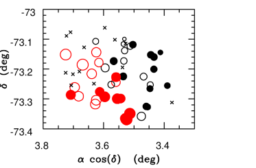
Figure 20: Velocity field of the nebular H ii. The size of symbol is proportional to the value of the velocity. Values greater than 155 km s^-1 are in red (electronic version only). Filled symbols are for binary systems while open symbols are for skies. Crosses are for binary systems showing no emission.

It is worth mentioning that the observed bimodal distribution of H ii is compatible with the kinematic study of H i in the SMC by Stanimirović et al. (SSJ04 (2004)), even though the gas we see in our work is certainly hotter than the gas observed at 21 cm wavelength. Indeed, the authors mention the existence of a bimodal velocity field with central velocities of 137 and 174 km s^-1. Interestingly, Fitzpatrick (elF85 (1985)) already mentioned two H i complexes with velocities 134 and 167 km s^-1, which our emitting gas is probably related with. Figure 20 shows the mean (heliocentric) velocity field obtained from nebular H ii data. Filled and open symbols correspond to binary and sky (nebular) data, respectively. The size of the symbol is drawn according to the value of the radial velocity. A cross indicates the position of a binary without significant emission. The map has the same orientation as in Fig.1. We can tentatively draw an oblique line from the NE to the SW corner demarcating high-velocity points from low-velocity points. This line has a $\sim 60\degr$ slope in the EN (clockwise) direction. On the east (i.e. left) side of this line, nebular RVs are greater than $\sim 155\leavevmode\nobreak\ \mathrm{kms^{-1}}$. This velocity gradient is consistent with Fig. 3 in Stanimirović et al., i.e. the velocity of H i increases from west to east in this part of the SMC. Therefore, the hot and cool phases of the gas seem to share very similar spatial and kinematic distributions.

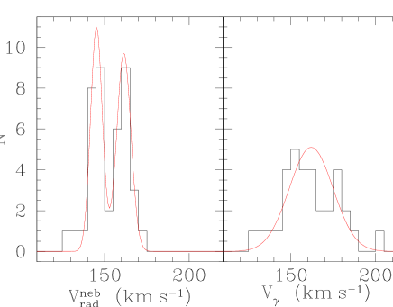
Figure 21: Comparison between two kinematic tracers: radial velocities of nebular H ii (left) and systemic velocities of binary systems (right). The data are arranged in 5 km s^-1 bins. The best-fitting double-Gaussian and Gaussian models are over-plotted.

Table 8: Sky positions: astrometry, sky background excesses (see Section 5.2) and mean radial velocities derived from the H$\gamma$ emission line.

id	$\alpha$ (J2000)	$\delta$ (J2000)	$\Delta_{\mathrm{sky}}$	$V_{\mathrm{rad}}$
	($\degr$)	($\degr$)	(%)	(km s-1)
S1	12.20608	$-73.17275$	$+3.8\pm 5.4$	$143.9\pm 4.2$
S2	12.68487	$-73.18533$	$+13.4\pm 4.1$	$169.4\pm 5.8$
S3	12.43554	$-73.19611$	$-5.8\pm 4.7$	$152.8\pm 3.7$
S4	12.49946	$-73.14372$	$-4.8\pm 3.8$	$160.0\pm 4.4$
S5	12.49446	$-73.17817$	$+0.5\pm 7.0$	$155.8\pm 6.2$
S6	12.34712	$-73.24400$	$-11.4\pm 2.0$	$156.0\pm 3.7$
S7	12.40693	$-73.25211$	$-3.5\pm 1.5$	$145.2\pm 5.5$
S8	12.63725	$-73.31728$	$+19.8\pm 5.4$	$161.9\pm 2.4$
S9	12.61700	$-73.30436$	$+7.1\pm 5.5$	$162.2\pm 6.5$
S10	12.60371	$-73.21592$	$-6.8\pm 3.2$	$161.4\pm 7.3$
S11	12.83250	$-73.26103$	$+15.9\pm 3.8$	$160.9\pm 6.1$
S12	12.48021	$-73.10711$	$+4.2\pm 3.1$	$141.1\pm 2.7$
S13	12.85400	$-73.15156$	$+34.9\pm 7.3$	$168.2\pm 6.6$
S14	12.80883	$-73.29111$	$-1.5\pm 2.7$	$161.0\pm 3.9$
S15	12.17254	$-73.13839$	$-6.0\pm 3.4$	$142.8\pm 2.9$
S16	12.09937	$-73.12347$	$-5.7\pm 3.0$	$143.2\pm 1.1$
S17	12.16858	$-73.11614$	$+7.3\pm 5.5$	$134.9\pm 2.2$
S18	12.14775	$-73.09939$	$+10.2\pm 6.1$	$127.1\pm 1.5$
S19	11.95912	$-73.25294$	$+20.2\pm 5.2$	$142.1\pm 4.0$
S20	12.01675	$-73.22519$	$+25.4\pm 11.8$	$146.3\pm 3.2$
S21	12.13529	$-73.35828$	$-2.3\pm 6.8$	$154.3\pm 3.6$

5.3 Comparison with evolutionary models and the mass-luminosity relation

Comments on the individual systems were given in Section 4. Here, the collective properties of the sample are examined more thoroughly. For each of the 33 systems, Table 9 lists the differences $\Delta\mathcal{M}$ between the evolutionary mass interpolated, in the HR diagram, in the evolutionary tracks from Charbonnel et al. (CMMSS93 (1993)), and the observed dynamical mass determined from the simultaneous RV-curves and light-curves analysis. Figure 22 shows these differences versus the observed masses for the 23 binaries that have a detached configuration. The agreement between the observed and evolutionary masses is acceptable, though some systematics does appear. The most discrepant objects are the secondary components of 5 38089 and 5 123390, and the primary of 5 38089. These systems have a peculiar position in the HR diagram, perhaps because of third-light contamination.

For comparison, the sample of 18 detached systems of HHH05 is shown on Fig. 23. Figures 22 and 23 are drawn at the same scale. Beside the very large scatter of HHH05’s $\Delta\mathcal{M}$ values (they span a range of almost $10\leavevmode\nobreak\ \mathcal{M}_{\odot}$), the most striking feature is the correlation between $\Delta\mathcal{M}$ and the observed mass for a number of primary and secondary components, especially between $7$ and $15\leavevmode\nobreak\ \mathcal{M}_{\odot}$. Explaining this trend is not straightforward, but it might be related to the temperature determination. Indeed, HHH05 mention in their Section 3.1.2: “We found that the O—B1 stars were quite easy to classify, but that spectral classifications were more difficult for later B types due to the absence of He ii lines and, in these low metallicity stars, the lack of detectable Si ii and other metal lines”. We faced the same difficulty, but with much less severe consequences. The larger telescope and better resolution clearly have brought a dramatic improvement in the quality of the results.

There is a slight trend in our mass residuals: first of all, most $\Delta\mathcal{M}$ values are positive. Second, while the mass difference is negligible for low masses (around $4-5\leavevmode\nobreak\ \mathcal{M}_{\odot}$), it seems to gradually increase to almost $2\leavevmode\nobreak\ \mathcal{M}_{\odot}$ at about $13\leavevmode\nobreak\ \mathcal{M}_{\odot}$. The single point at $17\leavevmode\nobreak\ \mathcal{M}_{\odot}$ corresponds to $\Delta\mathcal{M}\sim 1\leavevmode\nobreak\ \mathcal{M}_{\odot}$ only, but it is not sufficient to define the possible relation beyond $13\leavevmode\nobreak\ \mathcal{M}_{\odot}$. It might be part of a parallel sequence defined by 4 other stars. One may speculate that, if real, the latter sequence might correspond to e.g. systems for which the sky background was overestimated, which would have caused an underestimate of $T_{\mathrm{eff}}$. The main trend is surprising, because the more massive systems are also more luminous on average and so appear brighter since they all lie at about the same distance. Hence the signal-to-noise ratio of their spectra is larger, and the determination of the $T_{\mathrm{eff}}$ should be more reliable. On the other hand, $T_{\mathrm{eff}}$ is better constrained in stars cooler than $\sim 20\,000$ K, because the He i lines increase in strength with increasing temperature, while the H i Balmer lines decrease. In hotter stars, both the H i and He i lines decrease with increasing temperature, so that even a slight error on the continuum placement or (equivalently) on the sky subtraction may cause a significant error on $T_{\mathrm{eff}}$. At the hot end of the temperature range of our sample (i.e. for $T_{\mathrm{eff}}>30\,000$ K), the effective temperature is again better constrained, thanks to the fast raise of He ii lines. Therefore, one may expect that the least reliable temperatures – hence the least reliable luminosities – will occur for stars with intermediate $T_{\mathrm{eff}}$ or masses. This might explain why the scatter of the $\Delta\mathcal{M}$ values in Fig. 22 is large between 7 and $14\leavevmode\nobreak\ \mathcal{M}_{\odot}$.

The fact that $\Delta\mathcal{M}>0$ in most cases is not easy to explain. Possible explanations can be grouped in three categories:

• Systematic error in the $T_{\mathrm{eff}}$ determination: As mentioned above, the temperature determination is very sensitive to continuum placement or sky subtraction, especially when all lines vary in the same way with $T_{\mathrm{eff}}$. The continuum has been determined both automatically and manually for each star, and we have verified that the least-squares fit used to determine the temperature always gives the same result, unless the continuum is clearly wrong. All fits were done under visual monitoring, so the quality of the continuum placement could be judged with confidence. In addition, plotting the estimated temperature against the sum of the squared residuals generally results in a horizontal line, as shown in Section 4 (the system 5 180576 is a notable exception). This is a proof that the $T_{\mathrm{eff}}$ determination does not depend on the SNR of the spectra or, in other words, that the continuum was defined in the same way, whatever the SNR of the spectrum. The normalisation, as well as the temperature determination, were done (in the so-called second step) on the original unsmoothed spectra. In order to further explore the possible role of the SNR, we smoothed the spectra of the system 4 121110 with a 3-points boxcar (0.6 Å  wide) and performed the $T_{\mathrm{eff}}$ determination again. The result was the same within $\sim 100$ K, which confirms that it is insensitive to the SNR of the spectra, since the latter, in this test, was improved by a factor of $\sqrt{3}$. Therefore, it is doubtful that the explanation resides in the way the continuum was defined.

  The sky subtraction may be more problematic. Indeed, we have seen that the sky does vary slightly in the FLAMES field, and all we could do was to subtract an average sky spectrum from the stellar spectra. Underestimating the sky would have left some continuum flux that would have slightly diluted the stellar absorption lines, leading to an overestimate of $T_{\mathrm{eff}}$. The only cure to this problem would have been to use the IFUs instead of the MEDUSA fibres, in order to be able, at least in principle, to measure the sky surrounding each object. But this would have been at the expense of a drastic reduction of the number of targets. Although sky subtraction can explain some of the scatter we see on Fig. 22, it remains to understand why it could lead to a systematic overestimate of $T_{\mathrm{eff}}$ (causing the overestimate of $L$ and, ultimately, of the interpolated $\mathcal{M}$). Since an average sky was subtracted, one would expect as many negative values of $\Delta\mathcal{M}$ as positive ones. However, the sky positions had been chosen, on the DSS chart, on the basis of their “darkness”, so that the selected skies may be darker than the ones that typically surround the targets.

• Inadequacy of the stellar evolution models: In Figs. 39–41, are plotted not only the evolutionary tracks for the metallicity $Z=0.004$ of Charbonnel et al. (CMMSS93 (1993)), but also those at $Z=0.001$ (Schaller et al. SSMM92 (1992)). It is interesting to see that the more metal-poor models are slightly more luminous and hotter, and some systems fit them better. It is possible that some stars have indeed a metallicity approching $Z=0.001$ (especially for the light elements, which are the main contributors to $Z$), as shown e.g. by Peters & Adelman (PA06 (2006)). However, it is doubtful that all our systems have such a low metallicity, and a look at the HR diagrams shows that this explanation cannot hold for all of them.

  Also plotted on Figs. 39–41 are the evolutionary tracks of Claret & Gimenez (CG98 (1998)) for a helium content $Y=0.28$ and a metallicity $Z=0.004$. These models have a helium enhancement $\Delta Y=0.028$ relative to those of Charbonnel et al. (CMMSS93 (1993)), since the latter have $Y=0.252$. One can see that increasing the helium content increases the luminosity, withouth changing the temperature. Again, some stars would fit better such models than the standard ones, while others (like the components of 4 175333) would need so large a helium enhancement as to make this solution untenable.

• Inadequacy of the synthetic spectra: If the true metallicity of most system is close to $Z=0.004$ and the helium content is normal, and if the standard evolutionary models can be trusted, then the synthetic spectra used to estimate the effective temperatures may be suspected. An overestimate of $T_{\mathrm{eff}}$ would certainly have resulted from the use of LTE atmosphere models: as shown by Hunter et al. (HDS07 (2007)) in their Table 13, the temperatures of stars analyzed by Kilian-Montenbruck et al. (KM94 (1994)), on the basis of LTE atmosphere models and non-LTE line formation calculations, are about $29\,000$ K, instead of $26\,000-27\,000$ K using NLTE models. Nevertheless, the synthetic spectra we used are precisely based on the latter, so that no obvious bias on temperatures is expected. Using the FASTWIND code, Massey et al. (MZM09 (2009)) found temperatures of O stars $\sim 1000$ K hotter than those obtained by Bouret et al. (BLH03 (2003)), who used the TLUSTY and CMFGEN codes. Part of the discrepancy might be explained, however, by moonlight continuum contamination in the spectra of Bouret et al. (BLH03 (2003)). On the other hand, Mokiem et al. (MKE06 (2006), MKE07 (2007)) found temperatures $\sim 1000$ K hotter than those of Massey et al. (MZM09 (2009)), while they also used FASTWIND. Finally, Massey et al. (MZM09 (2009)) still find some amount of mass discrepancy for their LMC stars. Therefore, some debate still exists regarding the temperature scales, though the above references all deal with O stars, rather than with the B stars we are more concerned with. Unfortunately, similar studies for metal poor B stars in the range we are interested in ($20\,000<T_{\mathrm{eff}}<30\,000$ K) are lacking, so it is difficult to assess the reliability of the temperature scale. One may expect, however, that it is more reliable than for O stars, since the NLTE effects are less important.

  The OSTAR2002/BSTAR2006 libraries we have used are recent and are probably the best available. The only reservation one could possibly raise is the choice of the microturbulence (2  km s^-1 for $T_{\mathrm{eff}}\leq 30\,000$ K and 10  km s^-1 for $T_{\mathrm{eff}}>30\,000$ K), which may be a rough approximation of reality.

  Conversely, even perfectly realistic models may prove inappropriate, if superficial abundance anomalies exist in the components of our binary systems. It is well known that early B-type stars may show a large overabundance of helium – the so-called helium-rich stars, of which HD 37776 is the prototype – but no example is known among components of close binaries. In any case, stronger He lines would mimick a lower effective temperature, while it seems that the temperatures are overestimated. Thus, only helium-weak stars could explain an overestimate of temperatures, but none are known at such high masses.

In conclusion, we consider the first explanation (sky subtraction problem) as the most probable one, until proven otherwise by other studies.

Table 9: Comparison with theoretical evolutionary models: difference between the evolutionary mass and the observed mass.

Object	Model	$\Delta\mathcal{M}_{\mathrm{P}}$	$\Delta\mathcal{M}_{\mathrm{S}}$
		($\mathcal{M}_{\odot}$)	($\mathcal{M}_{\odot}$)
4 110409	sd	1.076	1.923
4 113853	sd	1.500	0.855
4 117831	d	0.392	0.366
4 121084	d	1.503	1.404
4 121110	d	1.482	0.923
4 121461	d	0.731	0.429
4 159928	sd	1.089	0.566
4 160094	d	0.855	0.261
4 163552	d	0.222	0.197
4 175149	sd	4.143	5.091
4 175333	d	1.012	0.797
5 016658	d	0.296	0.646
5 026631	sd	0.924	0.459
5 032412	d	0.922	0.208
5 038089	d	1.764	2.349
5 095337	d	1.239	0.934
5 095557	d	1.215	0.639
5 100485	d	0.406	0.628
5 100731	c	0.248	0.686
5 106039	sd	0.807	1.119
5 111649	d	0.158	0.479
5 123390	d	1.236	2.574
5 180185	d	0.387	0.045
5 180576	d	1.119	0.082
5 185408	d	0.767	0.939
5 196565	d	0.446	0.241
5 261267	sd	1.921	1.569
5 265970	d	0.002	0.257
5 266015	sd	0.387	2.744
5 266131	d	0.637	0.447
5 266513	d	0.193	0.458
5 277080	sd	3.138	2.331
5 283079	d	0.704	0.674

Figure 22: Detached systems: difference between evolutionary mass and observed mass vs. observed mass. Filled symbols: primary; open symbols: secondary. The point in the inset, to the lower left corner, shows the median error bars for the mass of the primary. The vertical bar does not include the errors on luminosity and $T_{\mathrm{eff}}$ (hence on the interpolated mass), so it must be considered as a lower limit.

Figure 23: Same as Fig. 22, for the detached systems of Hilditch et al. (HHH05 (2005)).

The astrophysical parameters of our sample of detached binaries allow us to give a mass-luminosity relation for the SMC valid for masses between $\sim$4 and $\sim$18 $\mathcal{M}_{\odot}$. A linear regression fit gives, on all 46 points:

$$\log L/L_{\odot}=(3.04\pm 0.11)\log\mathcal{M}/\mathcal{M}_{\odot}+(0.90\pm 0.09)$$ (29)

with a RMS of $0.095$ (see the red line on Fig. 24). This is almost exactly the same relation as that obtained by Gonzáles et al. GOMM05 (2005) for the LMC. The mass-luminosity diagram is plotted in Fig. 24 together with the isochrones computed from the Geneva models for $Z=0.004$ and $Y=0.252$ (Charbonnel et al. CMMSS93 (1993)). All objects are, within the $1\,\sigma$ uncertainty, on or above the theoretical zero-age main sequence.

Most stars lie below the 50 Myr isochrone. The exceptions are some low-mass objects ($\lesssim 6\mathcal{M}_{\odot}$), i.e. both components of 5 111649 and of 4 175333. These two systems appear to be $\gtrsim$70 Myr old. They clearly bias the regression line to a low value of the slope. Graczyk (dG03 (2003)) adopts the relation

$$\log L/L_{\odot}=(3.664\pm 0.047)\log\mathcal{M}/\mathcal{M}_{\odot}+(0.380\pm 0.027)$$

for the LMC and the SMC, which is shown as the full blue line in Fig. 24. The latter relation appears slightly too steep: it clearly runs above unevolved stars with $\mathcal{M}\gtrsim 8-10\leavevmode\nobreak\ \mathcal{M}_{\odot}$.

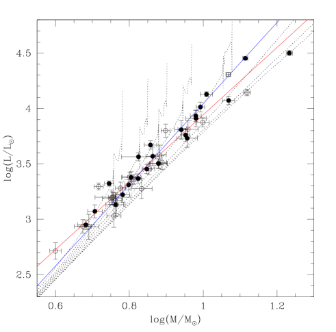
Figure 24: The mass-luminosity relation for our 23 detached systems. Full dots represent the primary components, while open dots represent the secondary ones. The dotted lines are the isochrones with age of 0, 5, 10, 20, 30, 40, 50 and 70 Myr for $Z=0.004$ (Charbonnel et al. CMMSS93 (1993)). The red line is a simple least-squares fit of all 46 points, without weighing. The steeper blue line is the relation adopted by Graczyk (dG03 (2003)) for the LMC and SMC.

5.4 Apsidal motion

Four of the nine eccentric systems have a negligible or marginal (i.e $\lesssim 2\,\sigma$) apsidal motion, while four others show a formally significant one (see Table 11); the apsidal motion of the ninth system was arbitrarily fixed to a value close to the theoretical expectation. Interestingly, the system 5 266131 has a very fast apsidal motion, and probably holds the record among those hosting non-degenerate components (Petrova & Orlov PO99 (1999), Bulut & Demircan BD07 (2007)). It is also worth noticing that in two of these systems (5 123390 and 5 266131), the relative radius of the primary component is very close to, or even slightly exceeds, the limiting radius above which orbital circularization occurs quickly (North & Zahn NZ03 (2003), NZ04 (2004)): they have $r_{p}=0.238$ and $0.281$ respectively, while the limiting radius is $\sim 0.25$. Thus, those systems are being caught in the act of circularizing their orbit, and indeed their eccentricities are among the smallest of all our eccentric binaries.

In order to compare our observed apsidal rotation rates with those predicted by theory, we used the equations (1) to (8) of Claret & Giménez (CG93 (1993)), which allow to obtain the average tidal–evolution constant $\bar{k_{2}}_{\mathrm{obs}}$ of the system from the orbital and stellar parameters, including the measured apsidal period $P_{\mathrm{apsid}}=2\pi/\dot{\omega}$. On the other hand, we used the grid of stellar models for the metallicity $Z=0.004$ computed by Claret (C05 (2005)). After interpolation in surface gravity and mass of the theoretical $\log(k_{2})$ values, the same formulae were used to obtain the predicted average constant $\bar{k_{2}}_{\mathrm{theo}}$. We corrected for the relativistic precession term, even though it is small for short periods (Mazeh tM08 (2008)), since it contributes for no more than 2% to the total precession period. The result is shown in Fig. 25, where we plot $\bar{k_{2}}_{\mathrm{obs}}$ as a function of $\bar{k_{2}}_{\mathrm{theo}}$. The one–to–one relation is the straight diagonal line, and 3 systems fall on or very close to it. Two other systems are clearly discrepant. One of the latter, 5 95557, has a formally significant, but small apsidal motion; the masses are not very precisely determined, which may explain part of the difference. It is quite possible that the apsidal motion of 5 95557 is affected by the gravitational perturbation of a small, unseen third companion. The other discrepant system, 5 123390. is only marginally so, since it is only $2\,\sigma$ away from the equality line. In any case, one has to keep in mind that the error bars shown represent lower limits to the real uncertainties, because they include only the error on the apsidal period, while errors on the masses and radii of the components also contribute. The latter errors certainly dominate in the case of 5 266131, which lies below the equality line. The open dot represents the system 5 265970, for which an apsidal motion close to the theoretical value was assumed.

Figure 25: Observed versus theoretical apsidal constant $\bar{k}_{2}$, averaged over the two companions of each binary system according to the prescriptions of Claret & Gimenez (CG93 (1993)). The internal structure models used are those of Claret (C05 (2005)) for the metallicity $Z=0.004$. The oblique line is the equality. The error bars reflect the uncertainty on $\dot{\omega}$ alone, so they represent lower limits to the real error. The open dot without error bar represents the system $5\;265970$, for which an arbitrary apsidal motion was assumed.

It would be easy, by reobserving with photometry the few systems showing significant apsidal motion, to strongly reduce the error bar on the average $\bar{k_{2}}_{\mathrm{obs}}$. Further spectroscopic data would be needed as well to obtain more precise masses and radii, in order to determine a meaningful value of $\bar{k_{2}}_{\mathrm{obs}}$. That would bring an additional constraint on the metallicity and on the extent of overshooting, for instance.

5.5 Distribution of the mass ratios of the detached systems: do binaries really like to be twins ?

From the 21 detached systems of the HHH03/05 sample, Pinsonneault & Stanek (PS06 (2006)) suggest that the proportion of massive detached systems with a mass ratio close to unity is far larger than what would be expected from a classic Salpeter-like ($p(q)\propto q^{-2.35}$) or a flat ($p(q)=\mathrm{const}$) $q-$distribution. This statement is based on two arguments. The first one is the striking difference between the median mass ratio of the detached sample ($q=0.87$) and of the semi-detached/contact sample ($q=0.65$). The surprising point is not the low $q-$value for the semi-detached sample, as this is expected for a post mass-transfer system, but rather the high proportion of systems with $q>0.85$ in the detached sample. Moreover, they argue that this difference is real, i.e. not due to an observational bias such as the easier detection of systems with components of similar size and brightness. Their argument is that, beside the detached binaries with $q>0.85$, there are two detached systems with a $q-$value as low as $\sim$0.55. Indeed, it seems to be a very strong argument in favour of the reality of a population of twins, because the observation of detached systems with such a low $q$ value would mean that the cut-off value of the $q$ distribution of the detached systems is small enough ($\lesssim 0.55$) to exclude an observational bias. Let us remind that the cut-off value is the $q$ value which marks the transition between a double-lined and a single-lined binary (SB2-SB1 transition), i.e. a function of the resolution and of the $S/N$, beside stellar parameters. Therefore, as our sample of 23 detached systems is comparable and even slightly larger than HHH03/05’s, this is an excellent opportunity to compare both statistics and thus to shed some light on the controversial topic of the $q$ distribution of detached and semi-detached/contact systems.

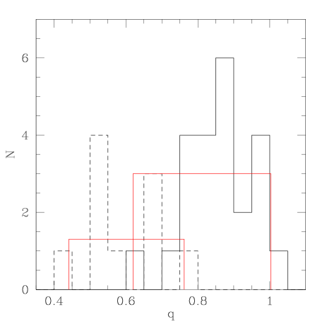
Figure 26: Distribution of the 33 observed mass ratios (solid: detached, dashed: semi-detached/contact) with 0.05 bins. The best flat distribution is over-plotted for each category (detached and semi-detached or contact systems). Both distributions are truncated at a cut-off value of $q\sim 0.7$ and $q\sim 0.4$, respectively.

The $q-$distributions for our detached and semi-detached/contact binaries are given in Fig. 26. One sees that the two samples have quite different distributions. The semi-detached/contact distribution is patchy because of the small size of the sample (10 objects), but it seems to be compatible with a constant law. The cumulative probability distribution of the mass ratios (Fig. 27, top) confirms that it is consistent with a flat distribution, limited to the interval $0.44<q<0.76$. The statistics of semi-detached system is not discussed by Pinsonneault & Stanek (PS06 (2006)). The subject was computationally investigated by van Rensbergen et al. (vRdLV (2005)). Interestingly, they mention that 80% of the observed Algols have a mass ratio in the 0.4-1 range. The low-value for this range coincides with the observed cut-off of our small sample. The problem is how to interpret this value. Through our experience in processing spectral data, we assume in this paper that this is the detection threshold for SB2 systems, but van Rensbergen et al. seem to consider this value not as an observational bias but rather as a parameter of real astrophysical relevance. Indeed, they have reproduced the observed Algolid $q-$distribution (from Budding et al.’s catalog eB04 (2004)) assuming a “liberal” model of evolution, i.e. a lot of mass loss and a little loss of angular momentum during mass transfer. Their simulations clearly depict a distribution with a broad peak in the 0.4-0.6 range and decreasing for higher $q-$values (see Fig. 5 in van Rensbergen et al. vRdLV (2005)). That is in excellent agreement with our results too. The only problem is one of their initial assumptions: they consider that the $q-$distribution of the detached Algol-progenitor systems obeys a Salpeter-like power law! That is not what we observe with our sample of 23 detached binaries. Figures 26 and 27 (top) show that the $q-$distribution of these systems is hardly compatible with a decreasing power law. Indeed, the data are very well modeled by a flat distribution truncated at $q=0.72$. The higher value for the SB1-SB2 cut-off compared to semi-detached systems is related to the almost $q^{3}-$dependence of the luminosity ratio for main-sequence stars. Let us mention that a flat $q-$distribution is assumed by most population synthesis studies (Pinsonneault & Stanek PS06 (2006)).

Figure 27: Top: cumulative probability distribution as a function of the mass ratio for our 23 detached (solid line) and 10 semi-detached/contact (dotted line) binaries. The dashed oblique line plotted over the detached distribution represents a flat distribution with a cutoff at $q=0.72$. In the case of the semi-detached/contact systems, a flat distribution with a cutoff at $q=0.43$ provides a reasonable fit as well. Bottom: cumulative probability distribution for HHH03/05’s 21 detached binaries. The over-plotted flat distribution with a cutoff at $q=0.5$ shows the incompatibility of a flat distribution with the HHH03/05 data. There is a similar figure in Pinsonneault & Stanek (PS06 (2006)). They show that the data are best-fitted with a 55% flat-45% twin distribution (not shown in this figure).

The cumulative probability distribution of the mass ratios for the HHH03/05 data is given in Fig. 27 (bottom). A similar figure is shown in Pinsonneault & Stanek. This distribution differs significantly from ours on two points: the low cut-off value of $\sim$0.5 and the relatively strong deviation from a flat distribution. The low cut-off is rather surprising. The mean apparent magnitude of the HHH03/05 sample ($\overline{I^{\mathrm{q}}}=15.47$ mag) is 1.38 mag lower than ours ($\overline{I^{\mathrm{q}}}=16.85$ mag). A rough estimation of the ratio of our mean $S/N$ to their mean $S/N$, taking into account our 2-times bigger telescope and longer exposure time via Eq. 3.2 of Hilditch (rH01 (2001)), gives a ratio of $\sim$0.8. That means that our mean spectral $S/N$ is 20% smaller than theirs despite the bigger optics because of significantly fainter targets. Nevertheless, their 20%-better $S/N$ hardly explains a luminosity ratio cut-off of $\sim$1/8 to be compared with our $\sim$1/3-value (for detached main-sequence binaries, $\mathcal{L}\sim q^{3}$). Moreover, the instrumental resolution of the LR2 setup in MEDUSA mode is 3-times the value of the 2dF spectrograph with the 1200B grating. Therefore, either our sample is deficient in low-$q$ systems or there are some badly determined $q-$values in one of the samples. The first explanation cannot be entirely ruled out because of the small-sample statistics. Nevertheless, the comparison of the RV-related parameters for the five systems common to both HHH03/05’s program and ours can certainly help to settle the issue.

Can the “twin hypothesis” be excluded by our data? The thorough study by Lucy (L06 (2006)) points to a negative answer. He discusses both the “weak” hypothesis ($\mathcal{H}_{w}$) of an excess of binary systems with $q>0.8$ relative to a constant distribution, and the “strong” hypothesis ($\mathcal{H}_{s}$) of an excess of systems with $q>0.95$. He shows that $\mathcal{H}_{s}$ is confirmed for binary systems in our Galaxy with an accurate enough mass ratio ($\sigma_{q}<0.01$). Therefore, it would be of great interest to test the same hypothesis in another galaxy, and our study might, at first sight, be considered a second step towards that goal, after HHH03/05. But a realistic typical error on our $q$ values is $\sim 0.05$, and our sample of 15 systems with $q>0.84$ is so small, relative to the 102 systems used by Lucy, as to make impossible any confirmation or rejection of $\mathcal{H}_{s}$. Our data might be more useful to constrain $\mathcal{H}_{w}$, but extensive simulations would be necessary to estimate the detection biases, and such an effort does not appear justified by our small sample. Therefore, the twin hypothesis remains an open question as far as the SMC (and any galaxy other than ours) is concerned.

5.6 Extinction and distances

5.6.1 Colour excess and extinction

The histogram of the 28 colour excesses is given in Fig. 28. Note that one system (5 196565) does not have $B$ and $V$ light curves and four systems have an unreliable observed $B-V$ index (see Section 3.3). The mean value is $\overline{E}_{B-V}=0.134\pm 0.051$ mag with individual values in the range 0.052-0.252 mag. By comparison, for four stars in the bar, Gordon et al. (GCMLW03 (2003)) found values ranging from 0.147 to 0.218 mag. From their extinction map across the SMC, Zaritsky et al. (ZHTGM02 (2002)) give $E_{B-V}\sim$0.05-0.25 mag. Sasselov et al. (dS97 (1997)) found a mean value of $\overline{E}_{B-V}=0.125\pm 0.009$ mag. Thus, our results are in very good agreement with these previous determinations. In order to investigate the spatial variation of the extinction across the studied field, $E_{B-V}$ was plotted against $\theta$, the distance to the optical center along the projected axis (not shown). No correlation was found. The GIRAFFE field is likely too small to detect a trend, if any.

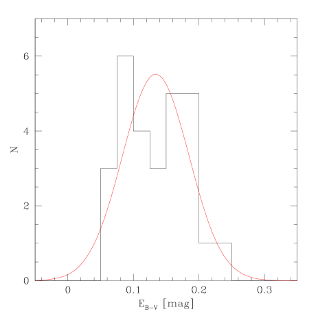
Figure 28: Histogram of colour excesses of 32 binaries in 0.025 bins. The best Gaussian fit is over-plotted.

5.6.2 Distance

The parameters relevant to the determination of the distance moduli are shared between Tables 4 (synthetic photometry) and 15. The DM was computed in both $V-$ and $I-$band, as explained in Section 3.12. One system (5 196565) has no value because of only one light curve available. Fortunately, for most systems the difference between the two computations of the individual DM is low and well within the uncertainties. As expected in Section 3.12, the $I-$values have a slightly lower absolute uncertainty. The discrepancy between the $V$ and $I$ moduli is negligible: $\overline{\Delta_{V-I}}\simeq-0.01$ mag with a scatter $\sigma=0.02$ mag for the 28 reliable systems.

The DMi were checked for a possible dependence upon a number of parameters: apparent visual magnitude, absolute visual magnitude, systemic velocity, colour excess and distance to the optical center along the projected axis. Statistical tests were performed (calculus of the Spearman rank correlation coefficient, followed by a Student T test) and no significant correlation was found. The $DM_{V}$ vs. $M_{V}^{\mathrm{q}}$ and $DM_{V}$ vs. $V^{\mathrm{q}}$ diagrams are shown in Fig. 29 (bottom). In order to calculate an unbiased mean DM, the HR diagrams (Fig. 39-41) of the individual systems were used to select the systems suitable for this purpose. This is actually a more objective criterion than relying solely on the quality of the light curves and spectra. Therefore, 8 objects showing strong discrepancies with theoretical models were conservatively discarded from the sample of 27 binaries (which remain from the initial sample of 33 binaries, after suppression of stars with unreliable or no colour index, or with a 3rd light, see below). Some of the primaries of these 8 systems may have luminosities really higher or lower than expected, but we can lucidly assume that most discrepancies are the direct consequences of low $S/N$ data and/or third light contamination. These suspicious systems are indicated by open symbols in Fig. 29.

From the sample of 33 objects, six at least must be discarded for the computation of the mean distance modulus: 5 196565 because of the total lack of $B$ and $V$ data, 4 163552 because of a third light contribution, and 4 systems which do not have reliable observed colour indices (5 038089, 5 180185, 5 261267 and 5 277080). At that stage, there remain 27 systems with presumably good distance moduli, without consideration of their HR diagrams. Removing further the 8 systems which have a dubious position in the HR diagram (i.e. 4 113853, 4 121084, 4 121110, 4 175149, 4 175333, 5 95557, 5 123390 and 5 185408) leaves us with only 19 systems, a bit more than half of the initial sample. By “dubious position”, we mean systems for which the error bar of the mass does not overlap that of the luminosity/temperature on the HR diagram. A third subsample was defined, which contains the nine “best” systems, defined as those detached systems for which, either the luminosity/temperature error bar overlaps the $Z=0.004$ evolutionary track, or the mass error bar overlaps the representative point of the corresponding component, for at least one of the components. These systems are 4 121461, 4 160094, 5 16658, 5 32412, 5 100731, 5 111649, 5 265970, 5 266131 and 5 266513.

Another important point is to identify possible biases acting upon the DM distribution. Actually, there is a small magnitude cut-off. This is the apparent magnitude cut-off, close to $V^{\mathrm{q}}\sim 18.1$ mag. It almost coincides with the apparent magnitude of 5 266513, the faintest binary of our sample, whose spectra have (smoothed) $S/N$ in the 18-50 range. This $V$ cut-off sets a higher limit for the absolute magnitude a binary should have in order to be seen across the whole depth of the SMC field. If we take $\sim$19.5 as the upper limit for the DM, then we find that the $M_{V}^{\mathrm{q}}$cut-off is $-1.82\pm 0.16$ mag with $\overline{E}_{B-V}=0.134\pm 0.051$ mag. The cut-off strip for $V^{\mathrm{q}}=18.1$ mag is indicated in Fig. 29 (bottom-left). Systems to the right of the oblique lines are too faint to be observed as SB2 with good enough spectra.

For example, in spite of a reliable solution, the binary 4 175333 should be discarded from the calculus of the mean DM in order to remove the observational bias just discussed. Indeed, with $M_{V}^{\mathrm{q}}=-1.217$ and $(V-M_{\mathrm{V}})_{0}=18.61$, this system would not be perceived as an SB2 if it were more distant, i.e. if it had $(V-M_{\mathrm{V}})_{0}\gtrsim 19.0$ (see Fig. 29, bottom-left). In fact this object had already been discarded on the basis of the peculiar position of its components in the HR diagram.

At the other end of the $M_{V}^{\mathrm{q}}-$ spectrum, there is a second cut-off, but this one does not bias the DM-distribution. This is the cut-off of the luminosity function, responsible for the depleted left-part of Fig. 29 (bottom-right). Close to $M_{V}^{\mathrm{q}}\sim-4.2$ mag, this is roughly the low-limit for late O stars: intrinsically brighter stars should be earlier O stars, but they are very scarce, so the probability of finding one in a sample of 33 objects is very low.

The histograms of the individual DMi in $V$ and $I$ are shown in Fig. 29 (top-left). For a given band, both the whole sample (i.e. the 27 systems remaining after the exclusion of the obviously problematic ones) and the “good systems” (i.e. the 19 best ones) distributions are plotted. Although 8 systems are considered as less reliable, one can see that all but three (4 175149, 4 175333 and 5 123390) discarded values are within the “good systems” range of DMi. This range spans 0.45 mag, from 18.87 to 19.32. The modes of the $V$ and $I$ distributions of the “good systems” are 19.15 and 19.20 respectively. In addition the distribution of the 9 “best” systems is plotted in red.

One can wonder how far the average value of the DMs is the most pertinent indicator of the mean distance of our stars. There is a $\sim 0.05$ to $0.1$ mag deviation between the modal and mean values of the distributions (for both $V$ and $I$), but we verified that these distributions, in spite of their apparent asymmetry, do not depart from gaussians in a significant way. Since the modal value is not a robust one for such small samples, we rather considered the weighted average and the median values.

The average and median distance moduli for the three subsamples defined above are given in Table 10 for the $V$ and $I$ bands. The average values are weighted by the reciprocal variance of the individual moduli. The RMS scatter is given beside each average value; beside each median value is given the width of the distribution, defined as the half difference between the upper and lower quartiles.

Table 10: Summary of the average and median distance moduli, for the three subsamples defined in the text. The given uncertainties represent the RMS scatters, not the errors on the respective average distance moduli.

Subsample	Stat. type	$\overline{(V-M_{\mathrm{V}})_{0}}$	$\overline{(I-M_{\mathrm{I}})_{0}}$
all 27	w. average	$19.07\pm 0.19$	$19.07\pm 0.19$
	median	$19.11\pm 0.12$	$19.11\pm 0.12$
19 good	w. average	$19.10\pm 0.14$	$19.11\pm 0.14$
	median	$19.13\pm 0.10$	$19.12\pm 0.13$
9 best	w. average	$19.10\pm 0.15$	$19.12\pm 0.16$
	median	$19.13\pm 0.07$	$19.12\pm 0.07$

We see that the $V$ and $I$ distance moduli of any given subsample are perfectly consistent. More surprisingly, the sample of all 27 systems has a slightly shorter distance modulus than the two other subsamples, while it contains many systems with large positive $\Delta\mathcal{M}$ values (see Section 5.3). Likewise, the sample of the 9 best systems (i.e. those which match the standard $Z=0.004$ evolutionary tracks best) have the same distance modulus as the sample of the 19 good systems. These results suggest that the components which are overluminous with respect to their $Z=0.004$ track are not necessarily overluminous in reality. Otherwise, if their luminosity were overestimated, they should also lie at a larger apparent distance.

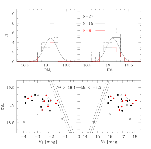
Figure 29: Top: distribution of the $V$- (left) and $I$-band (right) distance moduli. The distribution of the whole sample of 27 systems with good colours and presumably without 3rd light (dashed line) is shown. Only binaries with good HR diagrams are selected for the smaller statistics. The best fitting Gaussian curves for the 19-binary distributions are over-plotted. Bottom: distance modulus vs. absolute visual magnitude (left) and distance modulus vs. apparent visual magnitude (right). The estimated magnitude cut-off for a mean extinction is indicated by the diagonal solid line; the dashed lines correspond to the cut-off lines for $\overline{E}_{B-V}=0.134\pm 0.051$ mag. Ten binaries with dubious luminosities are shown with open symbols.

Finally, combining both $V$ and $I$ results, we adopt

$$\langle(m-M)_{0}\rangle=19.11\pm 0.03\;\;\;\;(66.4\pm 0.9\;\mathrm{kpc})$$ (30)

as the most probable average distance modulus for our sample. That value is $0.20\pm 0.03$ mag ($5.8\pm 0.9$ kpc) higher than the mean DM derived by HHH05, that is to say $18.912\pm 0.035$ (s.e.) ($60.59\pm 0.98$ kpc) from two samples totalizing 39 binaries. Our DM value does not agree HHH05’s, but contrary to theirs, it is not representative of the whole SMC. Our DM refers to the 25′-diameter GIRAFFE field at $\sim$0.45°  of the SMC optical center in a SW direction. Is this result coherent with the current knowledge of the 3-D structure of the SMC? The SMC bar is currently thought to be NE to SW-oriented, with the NE part closer to us than the SW part and the optical center occupying a mid position (Groenewegen mG00 (2000), HHH05). According to HHH05, there is a $\sim$2-3 kpc variation of the mean DM over their 2°  field. Given that gradient, our sample can be expected to be $\sim$0.5 kpc further than the optical center, since our field is $\sim$0.45°to the SW from it; but this difference is actually smaller than the uncertainty on our mean distance. If we took at face value the average distances moduli obtained by HHH05 and by us respectively, and assumed that HHH05 give a distance modulus representative of the SMC optical centre, one could in principle compute the real distance between the optical centre and the region corresponding to our field of view. Thus, taking into account the angular separation between the optical center and the center of the GIRAFFE field of view, the separation would correspond to $5.8\pm 1.3$ kpc along the SMC bar (see Fig. 1). That would mean that the bar is almost directed towards us, with a mean distance varying by as much as $25.8$ kpc over the $2^{\circ}$ covered by HHH05’s sample! Such a huge distance gradient, if real, would have been detected by Groenewegen mG00 (2000). Thus our larger distance cannot be reconciled with that obtained by HHH05. It is most probably due to the better observational material used here, as well as to the excellent synthetic spectra of Lanz & Hubeny (LH03 (2003), LH07 (2007)). On the other hand, our DM perfectly agrees with that obtained by Groenewegen (mG00 (2000)) using cepheids ($19.11\pm 0.11$ from the W index, and $19.04\pm 0.17$ from the K band). Taken at face value, our distance modulus clearly favors the so-called long distance scale.

5.6.3 Distance according to the detached systems versus distance according to the others

In the context of a search for systematic effects, one may wonder whether detached systems give a different distance modulus than the semi-detached or contact ones. Separating our 19 “good” systems into a group of 13 detached ones and a group of 6 semi-detached ones, we have computed the weighted average distance modulus (in the $I$ band) for each group. For the detached systems, we obtain $\overline{(I-M_{I})_{0}(d)}=19.07\pm 0.04$ mag, the error being the RMS scatter divided by $\sqrt{13}$. For the semi-detached and contact ones, we obtain $\overline{(I-M_{I})_{0}(sd,c)}=19.15\pm 0.05$ mag. Thus, our 6 semi-detached and contact systems are, on average, $0.08$ mag more remote than our 13 detached systems. Given the small statistics and the error bars, the difference is not significant since it amounts to only about $1.6\,\sigma$.

Nevertheless, we have looked at the distance moduli determined by HHH03/05, in order to see whether a similar difference exists in their data. Interestingly, almost the same difference appears: for 21 detached systems, one has $\overline{DM(d)}=18.85\pm 0.06$, while for the 29 others one has $\overline{DM(sd,c)}=18.91\pm 0.05$. So, here too, the semi-detached and contact systems are more remote than the detached ones on average, and by a similar amount, of $0.06$ mag. The effect is only of the order of $1\,\sigma$, so it is formally not significant. The coincidence between our results and those of HHH03/05 remains intriguing, however.

5.6.4 Depth

The observed dispersion of the DMi is the convolution of the true depth of our population of binaries with the average uncertainty on the DM determined for one binary system. Hence, under the assumption of a Gaussian distribution of both the cosmic and the error standard deviations, the true $1\,\sigma$ depth is given by the quadratic difference between the observed standard deviation of the moduli and the typical error on the modulus of an individual system. The observed standard deviation being 0.144 mag, and taking the average of the squares of the estimated errors as representative of the typical error, the $1\,\sigma$ depth becomes $\sqrt{0.144^{2}-0.00479}=0.126$ mag RMS ($\sim$3.9 kpc), since the average variance of an individual $I$ distance modulus is $0.00479$ mag². Groenewegen gives 0.11 mag (3.4 kpc) as the intrinsic $1\,\sigma$ spread for his sample of SMC Cepheids, so our result is in perfect agreement with his. The HHH05 sample (29 binaries) displays a higher dispersion, $\sim$0.28 mag ($\sim$7.8 kpc), but the authors consider that value as an overestimate. Our depth estimate is only 15% larger than that of Groenewegen (mG00 (2000)).

5.6.5 Temperature scale and distance modulus

We have seen that a suspicion remains, that the effective temperatures may have been overestimated in a number of systems. What is the effect of such an overestimate on the resulting distance modulus? For the sake of simplicity, let us consider a single star rather than a binary system. Its distance modulus can be written (under the assumption that we use the $V$ magnitude):

$$m-M = V_{q}+2.5\,\log\left(10^{-0.4\,M_{V}}\right)-3.1\,E_{B-V}$$

$$= \mathrm{const}+2.5\,\,\log\left(10^{-0.4\,(M_{bol}-BC)}\right)$$

$$-3.1\,\left[(B-V)_{q}-(B-V)_{0}\right]$$

since $V_{q}=\mathrm{const}$. Invoking Eqns. 3.11 and 16, which allow to express $(B-V)_{0}$ and $BC$ as a function of $T_{\mathrm{eff}}$, expressing the bolometric magnitude as a function of radius $R$ and $T_{\mathrm{eff}}$, and remembering that $(B-V)_{q}$ is constant for a given object, one obtains

$$m-M = \mathrm{const}\,+2.5\,\log\left(10^{-0.4\,\left[-5\log R-10\log T_{\mathrm{eff}}+\mathrm{cte}+5.51\log T_{\mathrm{eff}}\right]}\right)$$

$$-1.395\,\log T_{\mathrm{eff}}$$

$$= \mathrm{const}\,+3.095\,\log T_{\mathrm{eff}}$$

where we have taken into account that the radius is constant. Introducing a second star will essentially not change the result, because the ratio of the temperatures will appear (as well as the ratio of radii), which can be considered constant. Therefore, by differentiating the last equation above, one finally gets a very simple relation between a change $\Delta T_{\mathrm{eff}}$ of effective temperature, and the resulting change of the distance modulus:

$$\Delta(m-M)_{0}\simeq 1.344\,\frac{\Delta T_{\mathrm{eff}}}{T_{\mathrm{eff}}}$$ (31)

In the case of 4 175333, for instance, the temperature excess is especially large since it reaches $\sim 2000$ K. If the temperature is indeed overestimated, then the system is $\Delta(m-M)_{0}\simeq 1.344\times 0.092=0.123$ mag too far. Strangely enough, its modulus is only 18.60, so that it would be reduced to 18.48 under this assumption. The system 4 121110 has $\Delta T_{\mathrm{eff}}\sim 1580$ K and $\Delta(m-M)_{0}\sim 0.08$, so its modulus should be $19.00$ instead of $19.08$. Likewise, 4 121461 and 4 160094 have $\Delta(m-M)_{0}\sim 0.08$ and $0.06$ respecively, while they are listed as “good” systems.

A quick estimate of the average temperature excess of the 9 “best” systems leads to an average modulus excess of about $0.04$ mag, so that the corrected distance modulus would be reduced to 19.07, which still remains rather long compared to the frequently quoted value of $18.9$. In any case, it appears difficult to reduce the distance modulus to less than $19.0$. Thus, our data do favour the “long” rather than the “short” distance scale to the Magellanic Clouds.

6 Conclusions

The first goal of the present paper was to extract the fundamental stellar parameters characterizing 33 SB2 systems and then to test the reliability of stellar evolution models at low metallicity. We have shown that most components of detached systems have properties in fair agreement with the predictions of the Geneva single-star models at $Z=0.004$, although several systems appear slightly overluminous for their mass. From the subsample of detached systems, we give a mass-luminosity relation valid for masses between $\sim 4$ and $\sim 18\mathcal{M}_{\odot}$. Despite the lack of evolutionary cross checks, the semi-detached binaries appear to satisfy the typical morphology of Algol-like systems: a main-sequence primary with a large, less massive and more evolved secondary companion.

Our binaries were then used as primary standard candles. Average distance moduli obtained from the $I-$band data show no systematic difference compared to values obtained from the $V$ data. For each band, the frequency distribution of the DMi is not significantly different from a Gaussian. Combining $V$ and $I$ results and considering both the mean and the median values, we adopt $\langle(m-M)_{0}\rangle=19.11\pm 0.03$ as the average DM for the 19 most reliable systems. We have shown that, even if the effective temperatures are overestimated, so as to make the components of our systems overluminous relative to their mass, the average DM would still remain above $19.00$, so that our results support rather the long distance scale to the Magellanic Clouds than the short one. The true depth of our sample is estimated to be $2\times 0.126=0.25\leavevmode\nobreak\ \mathrm{mag}$ ($\sim$7.6 kpc), if we consider the $2\;\sigma$ interval as representative.

We have found a significant apsidal motion for at least three systems. For one system, the apsidal motion might be affected by an unseen third companion, but at least two other systems most probably owe it to the stellar structure of their components alone. The observed and predicted precession rates agree perfectly for the latter two systems, which are now circularizing their orbit, and the agreement extends to one or two other systems showing much less precise apsidal motion. The system 5 266131 shows probably the largest precession motion of all systems hosting main sequence stars, which is due exclusively to the non-point mass nature of the components.

Beside the astrophysical parameters and the distance moduli, other interesting results have been obtained. We have shown that the twin hypothesis for massive binaries is not supported by our results, although the latter are not strong enough to reject it either. Our sample of 23 detached systems agree quite well with a standard flat mass ratio spectrum. There is a clear cut-off of the $q-$distribution at $\sim 0.72$. Therefore, the high proportion of detached binaries having a $q$ value close to unity is more probably the result of an observational bias. The discrepancy observed by Pinnsonneault & Stanek (PS06 (2006)) may well be due to a number of underestimated mass ratios in the HHH03/05 sample. The distribution of the mass ratios of the semi-detached/contact binaries is consistent with a flat distribution restricted to the interval $0.4<q<0.8$. The sample is too small (10 objects) to tell more.

Another important result is the bimodal distribution of the radial velocity of the H ii gas, with peak values at $145.2\pm 0.5$ and $161.4\pm 0.6$ km s^-1.

Finally, we must emphasize that the accomplishment of this project was possible thanks to the public availability of the OGLE-II catalog of EB light curves, the OSTAR2002/BSTAR2006 libraries of synthetic spectra, the KOREL code and the PHOEBE interface to the WD codes.

Table 11: Orbital parameters: number of spectra used in the solution, minimum and maximum signal-to-noise ratio of the smoothed spectra, eccentricity, argument of the periastron for the epoch $t_{0}$ given in Table 3 and first derivative of it, inclination, semi-major axis, mass ratio, phase shift and systemic velocity.

Object	$n_{\mathrm{sp}}$	S/N	$e$	$\omega_{0}$ ($\degr$)	$i$	$a$	$q\equiv\mathcal{M}_{\mathrm{S}}/\mathcal{M}_{\mathrm{P}}$	$\Delta\phi$	$V_{\mathrm{\gamma}}$
				$\dot{\omega}$ ($\degr$ yr-1)	($\degr$)	($R_{\odot}$)			(km s-1)
4 110409	11	$65-140$	$0$	90	$77.3\pm 0.1$	$24.07\pm 0.20$	$0.524\pm 0.009$	$-0.00048\pm 0.00045$	$176.1\pm 1.3$
4 113853	7	$25-65$	$0$	90	$60.1\pm 0.3$	$10.95\pm 0.10$	$0.681\pm 0.011$	$-0.00447\pm 0.00125$	$134.1\pm 1.4$
4 117831	12	$28-71$	$0$	90	$78.2\pm 0.4$	$9.87\pm 0.06$	$0.981\pm 0.013$	$-0.00149\pm 0.00072$	$129.6\pm 1.1$
4 121084	9	$43-86$	$0$	90	$83.0\pm 0.1$	$10.30\pm 0.06$	$0.851\pm 0.009$	$-0.00246\pm 0.00035$	$147.2\pm 1.6$
4 121110	11	$52-95$	$0$	90	$81.9\pm 0.3$	$11.53\pm 0.06$	$0.747\pm 0.007$	$-0.00404\pm 0.00033$	$163.0\pm 1.1$
4 121461	15	$30-54$	$0.185$	$222.8\pm 1.4$	$81.1\pm 0.2$	$14.95\pm 0.08$	$0.961\pm 0.009$	$-0.04792\pm 0.00071$	$148.5\pm 0.8$
			$\pm 0.004$	$0.0$ (fixed)
4 159928	8	$50-108$	$0$	90	$61.1\pm 0.2$	$11.99\pm 0.12$	$0.556\pm 0.010$	$-0.00283\pm 0.00062$	$151.3\pm 2.0$
4 160094	11	$29-97$	$0.089$	$36.5\pm 6.7$	$77.0\pm 0.2$	$15.04\pm 0.24$	$0.752\pm 0.015$	$0.0170\pm 0.0006$	$149.0\pm 2.4$
			$\pm 0.007$	$9.8\pm 1.9$
4 163552	9	$73-132$	$0$	90	$80.9\pm 0.2$	$14.91\pm 0.19$	$0.952\pm 0.015$	$-0.00037\pm 0.00020$	$154.4\pm 2.4$
4 175149	15	1$17-168$	$0$	90	$78.8\pm 0.1$	$17.98\pm 0.22$	$0.659\pm 0.015$	$-0.00308\pm 0.00054$	$163.2\pm 2.2$
4 175333	14	$26-74$	$0.022$	$232.9\pm 15.8$	$80.4\pm 0.5$	$10.18\pm 0.09$	$0.781\pm 0.014$	$-0.00087\pm 0.00075$	$139.9\pm 1.4$
			$\pm 0.006$	$0.0$ (fixed)
5 016658	11	$30-62$	$0$	90	$80.3\pm 0.2$	$11.16\pm 0.09$	$0.889\pm 0.011$	$0.00002\pm 0.00035$	$158.6\pm 1.4$
5 026631	8	$77-120$	$0$	90	$61.4\pm 0.1$	$14.18\pm 0.11$	$0.690\pm 0.006$	$0.00264\pm 0.00051$	$150.8\pm 1.5$
5 032412	13	$58-92$	$0$	90	$83.4\pm 0.1$	$30.82\pm 0.14$	$0.767\pm 0.006$	$0.00014\pm 0.00019$	$177.4\pm 0.7$
5 038089	11	1$28-216$	$0$	90	$77.1\pm 0.2$	$21.88\pm 0.16$	$0.899\pm 0.011$	$-0.00047\pm 0.00039$	$152.9\pm 1.2$
5 095337	10	$48-89$	$0$	90	$88.8\pm 0.4$	$9.98\pm 0.08$	$0.874\pm 0.013$	$0.00278\pm 0.00033$	$183.8\pm 1.8$
5 095557	11	$33-75$	$0.218$	$155.7\pm 2.5$	$84.7\pm 0.3$	$17.54\pm 0.32$	$0.854\pm 0.026$	$0.00837\pm 0.00062$	$203.3\pm 2.6$
			$\pm 0.003$	$2.6\pm 0.5$
5 100485	13	$46-86$	$0$	90	$84.3\pm 0.2$	$13.12\pm 0.04$	$0.972\pm 0.006$	$-0.00109\pm 0.00026$	$159.2\pm 0.6$
5 100731	8	$35-74$	$0$	90	$59.7\pm 1.1$	$11.36\pm 0.16$	$0.762\pm 0.012$	$-0.01465\pm 0.00173$	$173.0\pm 1.6$
5 106039	9	$52-102$	$0$	90	$75.7\pm 0.1$	$16.81\pm 0.21$	$0.527\pm 0.012$	$-0.00182\pm 0.00041$	$153.3\pm 2.1$
5 111649	10	$52-89$	$0$	90	$74.4\pm 0.2$	$19.14\pm 0.11$	$0.936\pm 0.010$	$-0.00162\pm 0.00040$	$149.4\pm 0.8$
5 123390	14	$91-179$	$0.042$	$62.3\pm 5.2$	$74.3\pm 0.2$	$18.39\pm 0.19$	$0.804\pm 0.010$	$0.00470\pm 0.00046$	$141.7\pm 1.8$
			$\pm 0.006$	$4.8\pm 1.6$
5 180185	12	$37-64$	$0.036$	$88.6\pm 2.8$	$84.9\pm 0.2$	$29.91\pm 0.14$	$0.901\pm 0.009$	$-0.00182\pm 0.00051$	$165.2\pm 0.6$
			$\pm 0.005$	$0.0$ (fixed)
5 180576	12	$25-64$	$0$	90	$75.0\pm 0.4$	$13.31\pm 0.08$	$0.784\pm 0.009$	$0.00350\pm 0.00079$	$168.1\pm 1.0$
5 185408	12	$38-66$	$0$	90	$76.2\pm 0.3$	$12.69\pm 0.06$	$0.849\pm 0.008$	$-0.00141\pm 0.00057$	$174.9\pm 0.8$
5 196565	13	$44-86$	$0.138$	$231.9\pm 2.7$	$83.5\pm 0.2$	$24.65\pm 0.12$	$0.803\pm 0.007$	$-0.03068\pm 0.00038$	$162.3\pm 0.5$
			$\pm 0.006$	$1.2\pm 0.6$
5 261267	10	$41-88$	$0$	90	$89.7\pm 0.2$	$11.92\pm 0.08$	$0.525\pm 0.005$	$0.00289\pm 0.00018$	$176.0\pm 1.3$
5 265970	10	$67-111$	$0.054$	$362.5\pm 4.7$	$82.5\pm 0.1$	$24.67\pm 0.24$	$0.620\pm 0.008$	$0.01600\pm 0.00030$	$159.5\pm 1.3$
			$\pm 0.001$	$3.8$ (fixed)
5 266015	10	$69-118$	$0$	90	$78.5\pm 0.1$	$17.60\pm 0.09$	$0.441\pm 0.005$	$-0.00215\pm 0.00028$	$188.0\pm 1.1$
5 266131	10	$37-71$	$0.042$	$227.2\pm 2.3$	$83.5\pm 0.2$	$12.82\pm 0.15$	$0.864\pm 0.013$	$-0.00962\pm 0.00028$	$183.1\pm 2.6$
			$\pm 0.001$	$50.2\pm 2.0$
5 266513	10	$18-50$	$0$	90	$84.0\pm 0.4$	$9.91\pm 0.06$	$0.845\pm 0.010$	$-0.00073\pm 0.00056$	$164.4\pm 1.1$
5 277080	11	$74-130$	$0$	90	$76.6\pm 0.1$	$15.96\pm 0.13$	$0.504\pm 0.009$	$-0.00020\pm 0.00034$	$155.7\pm 1.3$
5 283079	10	$28-68$	$0$	90	$87.7\pm 0.3$	$12.28\pm 0.08$	$1.003\pm 0.013$	$0.00232\pm 0.00030$	$179.4\pm 1.3$

Table 12: Wilson-Devinney analysis, as obtained on the basis of both photometry and spectroscopy: system type (detached, semi-detached or contact), temperature ratio, normalized surface potentials and passband luminosity ratios. Third light contribution is given for the system 4 163552 (normalized to total flux at phase 0.25). The given potentials and the luminosity ratios are those obtained including the spectroscopic constraints (final WD/PHOEBE analysis).

Object	Model	$T_{\mathrm{eff}}^{\mathrm{S}}/T_{\mathrm{eff}}^{\mathrm{P}}$	$\Omega_{\mathrm{P}}$	$\Omega_{\mathrm{S}}$	$(L_{\mathrm{S}}/L_{\mathrm{P}})_{B}$	$(L_{\mathrm{S}}/L_{\mathrm{P}})_{V}$	$(L_{\mathrm{S}}/L_{\mathrm{P}})_{I}$	$(L_{\mathrm{S}}/L_{\mathrm{P}})_{B}^{\mathrm{sp}}$
					$\ell_{3,B}$	$\ell_{3,V}$	$\ell_{3,I}$
4 110409	sd	$0.654\pm 0.007$	$5.732\pm 0.092$	$2.922$ (fixed)	$1.292\pm 0.023$	$1.353\pm 0.024$	$1.367\pm 0.024$	$1.392\pm 0.036$
4 113853	sd	$0.737\pm 0.015$	$3.868\pm 0.090$	$3.209$ (fixed)	$0.680\pm 0.010$	$0.713\pm 0.009$	$0.753\pm 0.009$	$0.681\pm 0.058$
4 117831	d	$0.981\pm 0.023$	$4.855$ (fixed)	$4.479\pm 0.108$	$1.175\pm 0.052$	$1.177\pm 0.050$	$1.180\pm 0.049$	$1.009\pm 0.103$
4 121084	d	$0.940\pm 0.007$	$3.770$ (fixed)	$3.817\pm 0.043$	$0.707\pm 0.061$	$0.713\pm 0.010$	$0.720\pm 0.010$	$0.704\pm 0.061$
4 121110	d	$0.894\pm 0.007$	$3.820\pm 0.035$	$4.184\pm 0.059$	$0.424\pm 0.005$	$0.433\pm 0.005$	$0.442\pm 0.005$	$0.415\pm 0.047$
4 121461	d	$0.949\pm 0.023$	$6.980\pm 0.133$	$6.822\pm 0.099$	$0.907\pm 0.030$	$0.914\pm 0.029$	$0.923\pm 0.029$	$0.954\pm 0.063$
4 159928	sd	$0.723\pm 0.010$	$3.138\pm 0.024$	$2.983$ (fixed)	$0.357\pm 0.003$	$0.376\pm 0.003$	$0.397\pm 0.004$	$0.453\pm 0.029$
4 160094	d	$0.854\pm 0.018$	$5.517$ (fixed)	$5.545\pm 0.100$	$0.476\pm 0.050$	$0.489\pm 0.007$	$0.502\pm 0.007$	$0.428\pm 0.101$
4 163552	d	$0.997\pm 0.004$	$3.983\pm 0.026$	$4.214\pm 0.044$	$0.798\pm 0.024$	$0.799\pm 0.016$	$0.800\pm 0.014$	$0.926\pm 0.171$
					$0.142\pm 0.014$	$0.112\pm 0.012$	$0.119\pm 0.006$
4 175149	sd	$0.849\pm 0.006$	$4.411\pm 0.056$	$3.171$ (fixed)	$1.176\pm 0.025$	$1.200\pm 0.023$	$1.229\pm 0.023$	$1.415\pm 0.132$
4 175333	d	$0.879\pm 0.022$	$5.054\pm 0.151$	$5.010\pm 0.196$	$0.582\pm 0.034$	$0.595\pm 0.035$	$0.609\pm 0.036$	$0.562\pm 0.103$
5 016658	d	$1.007\pm 0.009$	$4.086$ (fixed)	$4.590\pm 0.068$	$0.609\pm 0.074$	$0.612\pm 0.008$	$0.614\pm 0.008$	$0.604\pm 0.074$
5 026631	sd	$0.734\pm 0.007$	$3.507\pm 0.030$	$3.226$ (fixed)	$0.495\pm 0.003$	$0.519\pm 0.003$	$0.547\pm 0.003$	$0.736\pm 0.049$
5 032412	d	$0.880\pm 0.008$	$7.284$ (fixed)	$6.949\pm 0.073$	$0.578\pm 0.050$	$0.584\pm 0.007$	$0.583\pm 0.007$	$0.546\pm 0.005$
5 038089	d	$1.012\pm 0.009$	$4.606\pm 0.047$	$5.065\pm 0.067$	$0.693\pm 0.019$	$0.692\pm 0.018$	$0.691\pm 0.018$	$0.678\pm 0.032$
5 095337	d	$0.936\pm 0.007$	$3.685\pm 0.022$	$3.835\pm 0.040$	$0.676\pm 0.008$	$0.684\pm 0.008$	$0.691\pm 0.008$	$0.659\pm 0.085$
5 095557	d	$0.908\pm 0.013$	$5.991\pm 0.107$	$6.602\pm 0.165$	$0.523\pm 0.015$	$0.532\pm 0.015$	$0.541\pm 0.015$	$0.625\pm 0.190$
5 100485	d	$1.008\pm 0.007$	$5.193\pm 0.076$	$5.216\pm 0.080$	$0.966\pm 0.034$	$0.965\pm 0.034$	$0.963\pm 0.034$	$0.930\pm 0.052$
5 100731	c	$0.828\pm 0.035$	$3.851\pm 0.058$	$3.351$ (fixed)	$0.517\pm 0.014$	$0.533\pm 0.013$	$0.552\pm 0.012$	$0.438\pm 0.041$
5 106039	sd	$0.638\pm 0.006$	$5.178\pm 0.057$	$2.928$ (fixed)	$1.007\pm 0.009$	$1.076\pm 0.009$	$1.168\pm 0.009$	$1.062\pm 0.063$
5 111649	d	$1.025\pm 0.011$	$4.600$ (fixed)	$4.736\pm 0.067$	$0.889\pm 0.056$	$0.886\pm 0.015$	$0.882\pm 0.014$	$0.880\pm 0.052$
5 123390	d	$1.017\pm 0.020$	$5.077$ (fixed)	$5.631\pm 0.106$	$0.587\pm 0.060$	$0.587\pm 0.011$	$0.585\pm 0.010$	$0.584\pm 0.061$
5 180185	d	$1.036\pm 0.029$	$7.724\pm 0.169$	$8.571\pm 0.249$	$0.707\pm 0.042$	$0.705\pm 0.025$	$0.700\pm 0.024$	$0.611\pm 0.042$
5 180576	d	$0.813\pm 0.027$	$4.918\pm 0.170$	$5.071\pm 0.207$	$0.450\pm 0.027$	$0.465\pm 0.028$	$0.483\pm 0.029$	$0.45\pm 0.07$
5 185408	d	$0.944\pm 0.018$	$5.052$ (fixed)	$4.957\pm 0.094$	$0.757\pm 0.047$	$0.764\pm 0.017$	$0.772\pm 0.016$	$0.619\pm 0.045$
5 196565	d	$0.867\pm 0.016$	$5.956$ (fixed)	$6.639\pm 0.120$	$0.43\pm 0.04^{\mathrm{a}}$	b	$0.453\pm 0.009$	$0.413\pm 0.040$
5 261267	sd	$0.728\pm 0.004$	$3.353\pm 0.013$	$2.923$ (fixed)	$0.439\pm 0.002$	$0.461\pm 0.003$	$0.487\pm 0.001$	$0.451\pm 0.039$
5 265970	d	$0.901\pm 0.012$	$4.157$ (fixed)	$5.370\pm 0.056$	$0.219\pm 0.024$	$0.264\pm 0.001$	$0.227\pm 0.001$	$0.233\pm 0.024$
5 266015	sd	$0.757\pm 0.005$	$3.512\pm 0.026$	$2.759$ (fixed)	$0.494\pm 0.002$	$0.515\pm 0.002$	$0.539\pm 0.002$	$0.617\pm 0.045$
5 266131	d	$0.936\pm 0.007$	$4.510$ (fixed)	$4.727\pm 0.065$	$0.647\pm 0.060$	$0.655\pm 0.008$	$0.661\pm 0.007$	$0.644\pm 0.060$
5 266513	d	$0.959\pm 0.018$	$4.390$ (fixed)	$4.530\pm 0.084$	$0.692\pm 0.070$	$0.697\pm 0.016$	$0.703\pm 0.015$	$0.733\pm 0.076$
5 277080	sd	$0.685\pm 0.004$	$3.932\pm 0.047$	$2.884$ (fixed)	$0.567\pm 0.015$	$0.600\pm 0.008$	$0.641\pm 0.008$	$0.690\pm 0.022$
5 283079	d	$0.997\pm 0.010$	$5.162$ (fixed)	$5.184\pm 0.074$	$0.987\pm 0.086$	$0.987\pm 0.015$	$0.988\pm 0.015$	$0.936\pm 0.088$

• $B$ data missing, ratio given by the WD code on the basis of the $I$ data, via the atmosphere models

• $V$ data missing

Table 13: Astrophysical parameters for the primary components: masses, radii, effective temperatures, surface gravities, luminosities and equilibrium equatorial velocity (i.e. synchronous velocity for circular systems and pseudo-synchronous velocity for eccentric systems).

Object	$\mathcal{M}_{\mathrm{P}}$	$R_{\mathrm{P}}$	$T_{\mathrm{eff}}^{\mathrm{P}}$	$\log g_{\mathrm{P}}^{\ \mathrm{a}}$	$\log L_{\mathrm{P}}/L_{\odot}^{\ \mathrm{b}}$	$V_{\mathrm{rot}}^{P}$
	($\mathcal{M}_{\odot}$)	(R⊙)	(K)	(dex cgs)		(km s-1)
4 110409	$13.93\pm 0.59$	$4.64\pm 0.14$	$32370\pm 816$	$4.25\pm 0.03$	$4.326\pm 0.051$	$79\pm 2$
4 113853	$6.03\pm 0.38$	$3.50\pm 0.12$	$23150\pm 761$	$4.13\pm 0.04$	$3.499\pm 0.065$	$134\pm 5$
4 117831	$4.81\pm 0.25$	$2.71\pm 0.08$	$19190\pm 389$	$4.26\pm 0.04$	$2.949\pm 0.044$	$118\pm 4$
4 121084	$11.72\pm 0.44$	$3.64\pm 0.09$	$31580\pm 552$	$4.39\pm 0.03$	$4.072\pm 0.038$	$223\pm 6$
4 121110	$9.55\pm 0.33$	$3.84\pm 0.07$	$28390\pm 767$	$4.25\pm 0.02$	$3.933\pm 0.050$	$175\pm 3$
4 121461	$6.05\pm 0.26$	$2.59\pm 0.10$	$22970\pm 783$	$4.40\pm 0.04$	$3.222\pm 0.068$	$67\pm 3$
4 159928	$11.27\pm 0.46$	$4.85\pm 0.12$	$29080\pm 870$	$4.12\pm 0.03$	$4.178\pm 0.056$	$213\pm 5$
4 160094	$9.05\pm 0.58$	$3.23\pm 0.15$	$27550\pm 1106$	$4.38\pm 0.05$	$3.730\pm 0.081$	$96\pm 4$
4 163552	$9.56\pm 0.61$	$5.06\pm 0.16$	$24400\pm 990$	$4.01\pm 0.04$	$3.910\pm 0.075$	$166\pm 5$
4 175149	$11.78\pm 0.47$	$4.85\pm 0.16$	$33100\pm 272$	$4.14\pm 0.03$	$4.402\pm 0.032$	$123\pm 4$
4 175333	$5.09\pm 0.23$	$2.41\pm 0.08$	$21800\pm 644$	$4.38\pm 0.03$	$3.071\pm 0.059$	$98\pm 3$
5 016658	$6.38\pm 0.39$	$3.57\pm 0.12$	$21390\pm 519$	$4.14\pm 0.04$	$3.378\pm 0.051$	$145\pm 5$
5 026631	$11.40\pm 0.34$	$5.19\pm 0.08$	$28670\pm 394$	$4.07\pm 0.02$	$4.212\pm 0.028$	$186\pm 3$
5 032412	$17.12\pm 0.34$	$4.74\pm 0.11$	$35410\pm 174$	$4.32\pm 0.02$	$4.500\pm 0.022$	$66\pm 2$
5 038089	$13.01\pm 0.20$	$5.98\pm 0.08$	$30660\pm 130$	$4.00\pm 0.01$	$4.452\pm 0.014$	$127\pm 2$
5 095337	$8.72\pm 0.36$	$3.68\pm 0.12$	$26990\pm 1250$	$4.25\pm 0.03$	$3.808\pm 0.085$	$206\pm 7$
5 095557	$6.68\pm 0.71$	$3.60\pm 0.10$	$23710\pm 363$	$4.15\pm 0.05$	$3.564\pm 0.036$	$75\pm 2$
5 100485	$6.67\pm 0.14$	$3.14\pm 0.06$	$22670\pm 498$	$4.27\pm 0.02$	$3.367\pm 0.042$	$104\pm 2$
5 100731	$8.73\pm 0.51$	$3.76\pm 0.18$	$24550\pm 473$	$4.23\pm 0.05$	$3.664\pm 0.054$	$168\pm 8$
5 106039	$8.69\pm 0.37$	$3.63\pm 0.08$	$26320\pm 335$	$4.26\pm 0.03$	$3.754\pm 0.029$	$84\pm 2$
5 111649	$5.56\pm 0.16$	$5.30\pm 0.11$	$17000\pm 168$	$3.74\pm 0.02$	$3.322\pm 0.024$	$91\pm 2$
5 123390	$9.83\pm 0.26$	$4.38\pm 0.14$	$27840\pm 549$	$4.15\pm 0.03$	$4.013\pm 0.044$	$102\pm 3$
5 180185	$6.28\pm 0.14$	$4.41\pm 0.14$	$18500\pm 400$	$3.95\pm 0.03$	$3.311\pm 0.046$	$41\pm 1$
5 180576	$7.30\pm 0.31$	$3.25\pm 0.14$	$25000\pm 1057$	$4.28\pm 0.04$	$3.568\pm 0.083$	$105\pm 5$
5 185408	$7.03\pm 0.21$	$3.05\pm 0.09$	$24170\pm 475$	$4.32\pm 0.03$	$3.453\pm 0.042$	$106\pm 3$
5 196565	$7.20\pm 0.28$	$4.93\pm 0.13$	$21530\pm 368$	$3.91\pm 0.03$	$3.670\pm 0.038$	$63\pm 2$
5 261267	$9.17\pm 0.39$	$4.32\pm 0.10$	$27930\pm 904$	$4.13\pm 0.03$	$4.008\pm 0.060$	$171\pm 4$
5 265970	$10.21\pm 0.39$	$7.14\pm 0.16$	$23280\pm 153$	$3.74\pm 0.03$	$4.128\pm 0.023$	$103\pm 2$
5 266015	$15.58\pm 0.31$	$5.84\pm 0.08$	$32120\pm 545$	$4.10\pm 0.02$	$4.512\pm 0.032$	$163\pm 2$
5 266131	$8.96\pm 0.23$	$3.60\pm 0.13$	$26510\pm 774$	$4.28\pm 0.03$	$3.760\pm 0.060$	$140\pm 5$
5 266513	$5.79\pm 0.35$	$2.84\pm 0.13$	$20800\pm 1167$	$4.30\pm 0.05$	$3.131\pm 0.106$	$130\pm 6$
5 277080	$9.68\pm 0.55$	$4.72\pm 0.09$	$29780\pm 480$	$4.08\pm 0.03$	$4.196\pm 0.032$	$123\pm 2$
5 283079	$7.56\pm 0.41$	$2.98\pm 0.08$	$25160\pm 475$	$4.37\pm 0.03$	$3.504\pm 0.041$	$118\pm 3$

• Computed from $g=\frac{G\mathcal{M}}{R^{2}}$

• Computed from $\log\frac{L}{L_{\odot}}=2\log\frac{R}{R_{\odot}}+4\log\frac{T_{\mathrm{eff}}}{T_{\mathrm{eff,\odot}}}$

Table 14: Astrophysical parameters for the secondary components: masses, radii, effective temperatures, surface gravities, luminosities and equilibrium equatorial velocity (i.e. synchronous velocity for circular systems and pseudo-synchronous velocity for eccentric systems).

Object	$\mathcal{M}_{\mathrm{S}}$	$R_{\mathrm{S}}$	$T_{\mathrm{eff}}^{\mathrm{S\ a}}$	$\log g_{\mathrm{S}}^{\ \mathrm{b}}$	$\log L_{\mathrm{S}}/L_{\odot}^{\ \mathrm{c}}$	$V_{\mathrm{rot}}^{S}$
	($\mathcal{M}_{\odot}$)	(R⊙)	(K)	(dex cgs)		(km s-1)
4 110409	$7.30\pm 0.36$	$7.81\pm 0.18$	$21170\pm 582$	$3.52\pm 0.03$	$4.041\pm 0.052$	$133\pm 3$
4 113853	$4.10\pm 0.28$	$3.79\pm 0.13$	$17060\pm 664$	$3.89\pm 0.04$	$3.038\pm 0.074$	$145\pm 5$
4 117831	$4.72\pm 0.25$	$2.77\pm 0.08$	$18830\pm 588$	$4.23\pm 0.04$	$2.936\pm 0.060$	$120\pm 4$
4 121084	$9.98\pm 0.39$	$3.28\pm 0.09$	$29680\pm 560$	$4.41\pm 0.03$	$3.875\pm 0.041$	$202\pm 6$
4 121110	$7.13\pm 0.26$	$2.85\pm 0.07$	$25010\pm 703$	$4.38\pm 0.03$	$3.455\pm 0.053$	$130\pm 3$
4 121461	$5.82\pm 0.26$	$2.59\pm 0.10$	$21790\pm 909$	$4.38\pm 0.04$	$3.131\pm 0.080$	$67\pm 3$
4 159928	$6.27\pm 0.30$	$4.07\pm 0.12$	$21030\pm 686$	$4.02\pm 0.03$	$3.462\pm 0.062$	$179\pm 5$
4 160094	$6.81\pm 0.45$	$2.63\pm 0.14$	$23500\pm 1059$	$4.43\pm 0.05$	$3.276\pm 0.091$	$78\pm 4$
4 163552	$9.10\pm 0.57$	$4.54\pm 0.15$	$24330\pm 992$	$4.08\pm 0.04$	$3.812\pm 0.077$	$149\pm 5$
4 175149	$7.76\pm 0.31$	$6.18\pm 0.20$	$28110\pm 306$	$3.75\pm 0.03$	$4.330\pm 0.034$	$156\pm 5$
4 175333	$3.98\pm 0.14$	$2.06\pm 0.07$	$19170\pm 741$	$4.41\pm 0.03$	$2.713\pm 0.074$	$84\pm 3$
5 016658	$5.67\pm 0.35$	$2.84\pm 0.11$	$21510\pm 553$	$4.29\pm 0.04$	$3.190\pm 0.057$	$115\pm 5$
5 026631	$7.86\pm 0.25$	$4.93\pm 0.08$	$21050\pm 355$	$3.95\pm 0.02$	$3.631\pm 0.033$	$177\pm 3$
5 032412	$13.14\pm 0.28$	$4.06\pm 0.11$	$31160\pm 315$	$4.34\pm 0.02$	$4.144\pm 0.029$	$57\pm 2$
5 038089	$11.70\pm 0.18$	$4.94\pm 0.07$	$31020\pm 301$	$4.12\pm 0.01$	$4.307\pm 0.021$	$105\pm 2$
5 095337	$7.62\pm 0.32$	$3.23\pm 0.12$	$25270\pm 1185$	$4.30\pm 0.04$	$3.581\pm 0.087$	$181\pm 6$
5 095557	$5.70\pm 0.64$	$2.86\pm 0.08$	$21530\pm 446$	$4.28\pm 0.05$	$3.198\pm 0.044$	$60\pm 2$
5 100485	$6.49\pm 0.13$	$3.06\pm 0.06$	$22840\pm 527$	$4.28\pm 0.02$	$3.359\pm 0.044$	$102\pm 2$
5 100731	$6.65\pm 0.40$	$3.23\pm 0.16$	$20300\pm 931$	$4.24\pm 0.05$	$3.201\pm 0.091$	$144\pm 7$
5 106039	$4.58\pm 0.22$	$5.46\pm 0.11$	$16800\pm 265$	$3.63\pm 0.03$	$3.328\pm 0.032$	$126\pm 2$
5 111649	$5.21\pm 0.15$	$4.89\pm 0.10$	$17420\pm 260$	$3.78\pm 0.02$	$3.295\pm 0.032$	$84\pm 2$
5 123390	$7.91\pm 0.22$	$3.31\pm 0.13$	$28320\pm 784$	$4.30\pm 0.04$	$3.800\pm 0.059$	$77\pm 3$
5 180185	$5.66\pm 0.13$	$3.60\pm 0.13$	$19170\pm 657$	$4.08\pm 0.03$	$3.197\pm 0.067$	$33\pm 1$
5 180576	$5.73\pm 0.25$	$2.65\pm 0.13$	$20310\pm 1090$	$4.35\pm 0.05$	$3.030\pm 0.103$	$86\pm 4$
5 185408	$5.97\pm 0.19$	$2.80\pm 0.08$	$22830\pm 640$	$4.32\pm 0.03$	$3.280\pm 0.055$	$97\pm 3$
5 196565	$5.78\pm 0.23$	$3.69\pm 0.13$	$18670\pm 461$	$4.07\pm 0.03$	$3.170\pm 0.052$	$47\pm 2$
5 261267	$4.81\pm 0.23$	$3.86\pm 0.10$	$20330\pm 666$	$3.95\pm 0.03$	$3.359\pm 0.061$	$153\pm 4$
5 265970	$6.33\pm 0.30$	$3.72\pm 0.15$	$20980\pm 340$	$4.10\pm 0.04$	$3.381\pm 0.044$	$54\pm 2$
5 266015	$6.86\pm 0.16$	$5.46\pm 0.08$	$24320\pm 438$	$3.80\pm 0.02$	$3.971\pm 0.034$	$153\pm 2$
5 266131	$7.74\pm 0.21$	$3.10\pm 0.12$	$24820\pm 750$	$4.35\pm 0.04$	$3.513\pm 0.063$	$120\pm 5$
5 266513	$4.90\pm 0.30$	$2.45\pm 0.13$	$19940\pm 1184$	$4.35\pm 0.05$	$2.931\pm 0.113$	$112\pm 6$
5 277080	$4.88\pm 0.29$	$5.13\pm 0.09$	$20410\pm 372$	$3.71\pm 0.03$	$3.612\pm 0.035$	$134\pm 2$
5 283079	$7.58\pm 0.41$	$2.97\pm 0.08$	$25160\pm 534$	$4.37\pm 0.03$	$3.501\pm 0.044$	$117\pm 3$

• Computed from $T_{\mathrm{eff}}^{\mathrm{S}}=(T_{\mathrm{eff}}^{\mathrm{S}}/T_{\mathrm{eff}}^{\mathrm{P}})_{\mathrm{phot}}T_{\mathrm{eff}}^{\mathrm{P}}$

• Computed from $g=\frac{G\mathcal{M}}{R^{2}}$

• Computed from $\log\frac{L}{L_{\odot}}=2\log\frac{R}{R_{\odot}}+4\log\frac{T_{\mathrm{eff}}}{T_{\mathrm{eff,\odot}}}$

Table 15: Distance determination: bolometric absolute magnitudes, bolometric corrections, visual absolute magnitudes, visual extinction and reddening-free distance modulus in the $V-$ and $I-$band. The $I-$band distance modulus is available only for systems for which the $B$ and $V$ magnitudes are available. The “q” superscript denotes values at quadrature.

Object	$M_{\mathrm{bol}}^{\mathrm{P\ a}}$	$M_{\mathrm{bol}}^{\mathrm{S\ a}}$	$BC_{V}^{\mathrm{P\ b}}$	$BC_{V}^{\mathrm{S\ b}}$	$M_{V}^{\mathrm{P\ c}}$	$M_{V}^{\mathrm{S\ c}}$	$E_{B-V}^{\mathrm{q\ d}}$	$A_{V}^{\mathrm{q\ e}}$	$5\log[$d$]-5_{V}^{\mathrm{\ f}}$	$5\log[$d$]-5_{I}^{\mathrm{\ g}}$
	(mag)	(mag)	(mag)	(mag)	(mag)	(mag)	(mag)	(mag)	(mag)	(mag)
4 110409	$-6.06\pm 0.13$	$-5.35\pm 0.13$	$-3.10\pm 0.06$	$-2.12\pm 0.07$	$-2.96\pm 0.08$	$-3.23\pm 0.07$	$0.207\pm 0.009$	$0.642\pm 0.029$	$19.06\pm 0.061$	$19.06\pm 0.057$
4 113853	$-4.00\pm 0.16$	$-2.85\pm 0.18$	$-2.36\pm 0.08$	$-1.60\pm 0.09$	$-1.64\pm 0.10$	$-1.25\pm 0.10$	$0.194\pm 0.009$	$0.601\pm 0.029$	$19.00\pm 0.078$	$18.99\pm 0.075$
4 117831	$-2.62\pm 0.11$	$-2.59\pm 0.15$	$-1.90\pm 0.05$	$-1.85\pm 0.07$	$-0.73\pm 0.08$	$-0.74\pm 0.09$	$0.064\pm 0.006$	$0.198\pm 0.018$	$18.99\pm 0.062$	$18.97\pm 0.061$
4 121084	$-5.43\pm 0.09$	$-4.94\pm 0.10$	$-3.06\pm 0.04$	$-2.93\pm 0.05$	$-2.37\pm 0.07$	$-2.00\pm 0.07$	$0.187\pm 0.005$	$0.580\pm 0.017$	$19.28\pm 0.051$	$19.27\pm 0.049$
4 121110	$-5.08\pm 0.12$	$-3.89\pm 0.13$	$-2.83\pm 0.06$	$-2.55\pm 0.07$	$-2.25\pm 0.07$	$-1.34\pm 0.08$	$0.158\pm 0.008$	$0.490\pm 0.023$	$19.08\pm 0.057$	$19.08\pm 0.054$
4 121461	$-3.30\pm 0.17$	$-3.08\pm 0.20$	$-2.34\pm 0.08$	$-2.22\pm 0.10$	$-0.96\pm 0.11$	$-0.86\pm 0.12$	$0.147\pm 0.009$	$0.456\pm 0.027$	$19.05\pm 0.083$	$19.09\pm 0.080$
4 159928	$-5.69\pm 0.14$	$-3.90\pm 0.15$	$-2.88\pm 0.07$	$-2.12\pm 0.08$	$-2.81\pm 0.08$	$-1.78\pm 0.09$	$0.168\pm 0.007$	$0.521\pm 0.021$	$19.29\pm 0.066$	$19.30\pm 0.064$
4 160094	$-4.57\pm 0.20$	$-3.44\pm 0.23$	$-2.77\pm 0.10$	$-2.40\pm 0.11$	$-1.80\pm 0.13$	$-1.04\pm 0.14$	$0.075\pm 0.009$	$0.233\pm 0.027$	$18.96\pm 0.102$	$18.97\pm 0.100$
4 163552	$-5.02\pm 0.19$	$-4.78\pm 0.19$	$-2.48\pm 0.10$	$-2.47\pm 0.10$	$-2.55\pm 0.10$	$-2.30\pm 0.11$	$0.187\pm 0.008$	$0.580\pm 0.026$	$18.35\pm 0.079$	$18.36\pm 0.077$
4 175149	$-6.26\pm 0.08$	$-6.07\pm 0.09$	$-3.15\pm 0.02$	$-2.79\pm 0.03$	$-3.11\pm 0.07$	$-3.29\pm 0.07$	$0.053\pm 0.007$	$0.164\pm 0.022$	$18.52\pm 0.057$	$18.54\pm 0.054$
4 175333	$-2.93\pm 0.15$	$-2.03\pm 0.19$	$-2.22\pm 0.07$	$-1.89\pm 0.09$	$-0.71\pm 0.09$	$-0.14\pm 0.11$	$0.070\pm 0.007$	$0.217\pm 0.022$	$18.61\pm 0.074$	$18.60\pm 0.072$
5 016658	$-3.70\pm 0.13$	$-3.23\pm 0.14$	$-2.17\pm 0.06$	$-2.19\pm 0.06$	$-1.53\pm 0.08$	$-1.04\pm 0.10$	$0.080\pm 0.006$	$0.248\pm 0.019$	$19.13\pm 0.068$	$19.15\pm 0.066$
5 026631	$-5.78\pm 0.07$	$-4.33\pm 0.08$	$-2.85\pm 0.03$	$-2.12\pm 0.04$	$-2.93\pm 0.04$	$-2.20\pm 0.05$	$0.105\pm 0.004$	$0.326\pm 0.013$	$19.13\pm 0.036$	$19.17\pm 0.034$
5 032412	$-6.50\pm 0.05$	$-5.61\pm 0.07$	$-3.32\pm 0.01$	$-3.03\pm 0.02$	$-3.18\pm 0.05$	$-2.58\pm 0.06$	$0.250\pm 0.006$	$0.775\pm 0.019$	$19.19\pm 0.044$	$19.22\pm 0.041$
5 038089	$-6.38\pm 0.04$	$-6.02\pm 0.05$	$-2.98\pm 0.01$	$-3.01\pm 0.02$	$-3.40\pm 0.03$	$-3.01\pm 0.04$	$0.057\pm 0.011$	$0.177\pm 0.034$	$18.89\pm 0.042$	$18.83\pm 0.032$
5 095337	$-4.77\pm 0.21$	$-4.20\pm 0.22$	$-2.72\pm 0.11$	$-2.57\pm 0.11$	$-2.05\pm 0.11$	$-1.64\pm 0.12$	$0.124\pm 0.016$	$0.384\pm 0.050$	$19.17\pm 0.097$	$19.21\pm 0.089$
5 095557	$-4.16\pm 0.09$	$-3.24\pm 0.11$	$-2.42\pm 0.04$	$-2.19\pm 0.05$	$-1.74\pm 0.07$	$-1.06\pm 0.07$	$0.116\pm 0.004$	$0.360\pm 0.013$	$19.19\pm 0.052$	$19.20\pm 0.051$
5 100485	$-3.67\pm 0.10$	$-3.65\pm 0.11$	$-2.31\pm 0.05$	$-2.32\pm 0.06$	$-1.36\pm 0.06$	$-1.32\pm 0.06$	$0.077\pm 0.009$	$0.239\pm 0.028$	$18.84\pm 0.052$	$18.87\pm 0.047$
5 100731	$-4.41\pm 0.13$	$-3.25\pm 0.23$	$-2.50\pm 0.05$	$-2.04\pm 0.11$	$-1.91\pm 0.11$	$-1.21\pm 0.14$	$0.106\pm 0.005$	$0.329\pm 0.016$	$19.28\pm 0.090$	$19.32\pm 0.089$
5 106039	$-4.63\pm 0.07$	$-3.57\pm 0.08$	$-2.66\pm 0.03$	$-1.56\pm 0.04$	$-1.97\pm 0.05$	$-2.01\pm 0.05$	$0.154\pm 0.010$	$0.477\pm 0.032$	$18.95\pm 0.050$	$18.95\pm 0.042$
5 111649	$-3.56\pm 0.06$	$-3.49\pm 0.08$	$-1.59\pm 0.02$	$-1.65\pm 0.04$	$-1.97\pm 0.05$	$-1.84\pm 0.05$	$0.177\pm 0.009$	$0.549\pm 0.028$	$18.86\pm 0.046$	$18.88\pm 0.040$
5 123390	$-5.28\pm 0.11$	$-4.75\pm 0.15$	$-2.78\pm 0.05$	$-2.83\pm 0.07$	$-2.50\pm 0.08$	$-1.92\pm 0.10$	$0.092\pm 0.015$	$0.285\pm 0.048$	$18.75\pm 0.078$	$18.76\pm 0.068$
5 180185	$-3.53\pm 0.12$	$-3.24\pm 0.17$	$-1.80\pm 0.05$	$-1.89\pm 0.08$	$-1.73\pm 0.08$	$-1.35\pm 0.10$	$0.067\pm 0.012$	$0.208\pm 0.036$	$19.45\pm 0.073$	$19.31\pm 0.067$
5 180576	$-4.17\pm 0.21$	$-2.82\pm 0.26$	$-2.54\pm 0.10$	$-2.04\pm 0.13$	$-1.63\pm 0.13$	$-0.79\pm 0.15$	$0.150\pm 0.013$	$0.465\pm 0.039$	$19.14\pm 0.106$	$19.13\pm 0.101$
5 185408	$-3.88\pm 0.11$	$-3.45\pm 0.14$	$-2.47\pm 0.05$	$-2.32\pm 0.07$	$-1.41\pm 0.07$	$-1.13\pm 0.09$	$0.100\pm 0.005$	$0.310\pm 0.015$	$19.12\pm 0.057$	$19.13\pm 0.056$
$5196565\ ^{\mathrm{g}}$	$-4.42\pm 0.09$	$-3.17\pm 0.13$	$-2.18\pm 0.04$	$-1.82\pm 0.06$	$-2.25\pm 0.07$	$-1.35\pm 0.09$
5 261267	$-5.27\pm 0.15$	$-3.65\pm 0.15$	$-2.79\pm 0.08$	$-2.04\pm 0.08$	$-2.48\pm 0.08$	$-1.61\pm 0.08$	$0.085\pm 0.009$	$0.263\pm 0.027$	$19.35\pm 0.068$	$19.29\pm 0.064$
5 265970	$-5.57\pm 0.06$	$-3.70\pm 0.11$	$-2.36\pm 0.02$	$-2.12\pm 0.04$	$-3.21\pm 0.05$	$-1.58\pm 0.09$	$0.078\pm 0.005$	$0.242\pm 0.016$	$19.25\pm 0.048$	$19.28\pm 0.046$
5 266015	$-6.53\pm 0.08$	$-5.18\pm 0.08$	$-3.08\pm 0.04$	$-2.46\pm 0.04$	$-3.45\pm 0.05$	$-2.71\pm 0.05$	$0.179\pm 0.005$	$0.555\pm 0.017$	$19.23\pm 0.038$	$19.25\pm 0.036$
5 266131	$-4.65\pm 0.15$	$-4.03\pm 0.16$	$-2.68\pm 0.07$	$-2.53\pm 0.07$	$-1.97\pm 0.10$	$-1.50\pm 0.11$	$0.136\pm 0.012$	$0.422\pm 0.036$	$19.11\pm 0.081$	$19.12\pm 0.075$
5 266513	$-3.08\pm 0.26$	$-2.58\pm 0.28$	$-2.10\pm 0.13$	$-1.99\pm 0.14$	$-0.98\pm 0.15$	$-0.58\pm 0.16$	$0.159\pm 0.012$	$0.493\pm 0.038$	$19.13\pm 0.118$	$19.11\pm 0.114$
5 277080	$-5.74\pm 0.08$	$-4.28\pm 0.09$	$-2.93\pm 0.04$	$-2.04\pm 0.04$	$-2.81\pm 0.05$	$-2.24\pm 0.05$	$0.225\pm 0.013$	$0.698\pm 0.042$	$18.52\pm 0.056$	$18.71\pm 0.046$
5 283079	$-4.01\pm 0.10$	$-4.00\pm 0.11$	$-2.56\pm 0.05$	$-2.56\pm 0.05$	$-1.45\pm 0.07$	$-1.44\pm 0.07$	$0.161\pm 0.005$	$0.499\pm 0.017$	$19.11\pm 0.054$	$19.07\pm 0.052$

• Computed from $M_{\mathrm{bol}}=-5\log\frac{R}{R_{\odot}}-10\log\frac{T_{\mathrm{eff}}}{T_{\mathrm{eff,\odot}}}+M_{\mathrm{bol,\odot}}$

• Interpolated from Lanz & Hubeny (LH03 (2003), LH07 (2007))

• Computed from $M_{V}=M_{\mathrm{bol}}-BC_{V}$

• Computed from $E_{B-V}=(B-V)-(B-V)_{0}$

• Computed from $A_{V}=\mathcal{R}_{V}E_{B-V}$ with $\mathcal{R}_{V}=3.1\pm 0.3$

• Computed from $5\log[d]-5=V^{\mathrm{q}}-M_{V}^{\mathrm{q}}-A_{V}^{\mathrm{q}}$ where $M_{V}^{\mathrm{q}}=-2.5\log\left(10^{-0.4M_{V}^{\mathrm{P}}}+10^{-0.4M_{V}^{\mathrm{S}}}\right)$

• Computed from $5\log[d]-5=I^{\mathrm{q}}-M_{V}^{\mathrm{q}}+(V-I)_{0}^{\mathrm{q}}-0.600\,A_{V}^{\mathrm{q}}$

• $B$ and $V$ light curves missing

Table 16: Light curves: ratio of the primary minimum to the RMS ($I-$band), RMS scatters and minimum chi-squared values from WD/PHOEBE code.

Object	$\Delta I_{\mathrm{minI}}/\sigma_{I}$	$\sigma_{I}$	$\sigma_{V}$	$\sigma_{B}$	Object	$\Delta I_{\mathrm{minI}}/\sigma_{I}$	$\sigma_{I}$	$\sigma_{V}$	$\sigma_{B}$
		(mag)	(mag)	(mag)			(mag)	(mag)	(mag)
4 110409	$\sim$65	0.016	0.028	0.042	5 100485	30.1	0.017	0.018	0.020
4 113853	9.3	0.017	0.019	0.025	5 100731	19.2	0.021	0.013	0.022
4 117831	10.8	0.028	0.018	0.025	5 106039	23.7	0.016	0.107	0.114
4 121084	34.6	0.019	0.013	0.016	5 111649	19.7	0.011	0.017	0.029
4 121110	31.7	0.015	0.016	0.024	5 123390	13.8	0.010	0.050	0.063
4 121461	10.5	0.031	0.025	0.017	5 180185	18.6	0.019	0.040	0.038
4 159928	18.7	0.013	0.008	0.009	5 180576	9.7	0.021	0.021	0.030
4 160094	12.5	0.019	0.008	0.011	5 185408	10.0	0.023	0.012	0.013
4 163552	46.1	0.009	0.011	0.017	$5196565\ ^{\mathrm{a}}$	21.0	0.017
4 175149	36.1	0.024	0.021	0.028	5 261267	49.7	0.017	0.052	0.024
4 175333	12.1	0.027	0.020	0.022	5 265970	33.4	0.012	0.015	0.016
5 016658	22.4	0.020	0.009	0.020	5 266015	49.2	0.012	0.018	0.015
5 026631	24.5	0.010	0.011	0.013	5 266131	7.8	0.019	0.026	0.101
5 032412	33.4	0.009	0.012	0.028	5 266513	15.5	0.034	0.020	0.025
5 038089	22.4	0.014	0.042	0.049	5 277080	43.1	0.013	0.027	0.100
5 095337	17.9	0.018	0.186	0.206	5 283079	26.5	0.020	0.017	0.024
5 095557	21.1	0.026	0.022	0.019

• $B$ and $V$ light curves missing

Table 17: Radial velocity curves: RMS scatters.

Object	$\sigma_{\mathrm{P}}$	$\sigma_{\mathrm{S}}$	Object	$\sigma_{\mathrm{P}}$	$\sigma_{\mathrm{S}}$
	(km s-1)	(km s-1)		(km s-1)	(km s-1)
4 110409	11.5	4.2	5 100485	6.1	4.4
4 113853	7.8	12.4	5 100731	7.0	17.4
4 117831	11.0	12.6	5 106039	8.1	12.2
4 121084	7.6	13.8	5 111649	4.3	5.5
4 121110	7.6	9.1	5 123390	8.4	14.1
4 121461	7.6	10.1	5 180185	4.0	2.9
4 159928	8.3	11.9	5 180576	8.0	12.8
4 160094	13.7	29.4	5 185408	7.1	12.7
4 163552	10.5	8.8	5 196565	5.7	9.5
4 175149	8.6	10.5	5 261267	7.3	13.5
4 175333	19.0	23.4	5 265970	12.8	11.8
5 016658	7.7	17.2	5 266015	5.2	9.8
5 026631	7.8	7.4	5 266131	9.9	8.4
5 032412	3.3	4.9	5 266513	14.6	9.8
5 038089	3.1	2.9	5 277080	8.3	8.0
5 095337	8.3	12.0	5 283079	12.4	11.7
5 095557	31.0	20.6

Figure 36: Mass–surface gravity diagrams: the positions of the primary and the secondary components are indicated by filled and open symboles, respectively. The dotted lines ares isochrones from Charbonnel et al. (CMMSS93 (1993)) at $Z=0.004$, with ages of 3, 5, 10, 20, 30, 40, 50 and 100 Myr. See text for comments on individual stars.

Figure 37: Same as Fig. 36, for 12 more stars.

Figure 38: Same as Fig. 36, for nine more stars.