Multiply-interacting Vortex Streets

Abstract

We investigate the behavior of an infinite array of (reverse) von Kármán streets. Our primary motivation is to model the wake dynamics in large fish schools. We ignore the fish and focus on the dynamic interaction of multiple wakes where each wake is modeled as a reverse von Kármán street. There exist configurations where the infinite array of vortex streets is in relative equilibrium, that is, the streets move together with the same translational velocity. We examine the topology of the streamline patterns in a frame moving with the same translational velocity as the streets which lends insight into fluid transport through the mid-wake region. Fluid is advected along different paths depending on the distance separating two adjacent streets. Generally, when the distance between the streets is large enough, each street behaves as a single von Kármán street and fluid moves globally between two adjacent streets. When the streets get closer to each other, the number of streets that enter into partnership in transporting fluid among themselves increases. This observation motivates a bifurcation analysis which links the distance between streets to the maximum number of streets transporting fluid among themselves. We also show that for short times, the analysis of streamline topologies for the infinite arrays of streets can be expected to set the pattern for the more realistic case of a finite array of truncated streets, which is not in an equilibrium state and its dynamic evolution eventually destroys the exact topological patterns identified in the infinite array case. The problem of fluid transport between adjacent streets may be relevant for understanding the transport of oxygen and nutrients to inner fish in large schools as well as understanding flow barriers to passive locomotion.

1 Introduction

This paper considers the interaction of multiple reverse von Kármán streets. The primary motivation is to model the wake dynamics in large fish schools and to gain insight into the role of the fluid in transporting oxygen and nutrients to inner fish as well as its role in facilitating or acting as flow barriers to passive locomotion.

We consider the parallel translational motion observed in fish schools and study the dynamic interaction of the multiple wakes. Each wake is modeled as a reverse von Kármán street and the fish producing the wakes are ignored. This model is reminiscent of the one employed in [20, 21] in analyzing the hydrodynamic advantages for fish schooling. The focus of [20, 21] was on investigating the energy-optimal positioning of an individual fish within the school (the famous diamond pattern) whereas in the present study, we focus on the interaction and fluid transport among multiple vortex streets for its relevance to understanding transport of nutrients as well as barriers to passive locomotion.

The classical von Kármán vortex street – made up of two rows of evenly spaced point vortices of equal and opposite sign staggered with respect to each other, see [6] – is the canonical ‘idealized’ vorticity configuration appearing generically in the wake of bluff bodies; see, for example, [22]. While the dynamics and stability of the single street is well-understood (see, for example, [3, 14] and references therein), little work is done on the interaction of multiple streets. An infinite array of streets can be viewed, under certain conditions on street alignments, as a special case of doubly-periodic vortex lattices whose Hamiltonian dynamics is investigated in [11, 17]; see also [12, 16] for investigations of singly-periodic lattices. Given the results in [17], one can argue that there exist configurations where an infinite array of streets is in relative equilibrium. This means that the streamline pattern remains steady in the frame moving with the same translational velocity as the streets. We look at the topology of the streamline patterns, that is to say, the streamline patterns relative to the moving frame, which lends insight into fluid transport through the mid-wake region. Fluid is advected along different paths depending on the distance separating two adjacent streets. Generally, when the distance between the streets is large enough, each street behaves as a single von Kármán street and fluid is transported globally between two adjacent streets. When the streets get closer to each other, the number of streets that enter into partnership in transporting fluid among themselves increases. This observation motivates a bifurcation analysis which links the distance between streets to the maximum number of streets transporting fluid among themselves.

An investigation of the stability of the relative equilibria in the infinite array of vortex streets is central to assessing the prevalence of the reported streamline topologies under spatial and temporal perturbations. The stability of a square lattice (of identical vortices) is addressed in the classical work of [18, 19]. Instead of casting the infinite arrays of streets as a Hamiltonian system following the methods developed in [11, 12, 16, 17] and studying its stability subject to periodic perturbations, we choose to examine the dynamics of a finite array of vortex streets. The finite array consists of vortex streets that are truncated horizontally (reflecting the fact that in real flows viscosity diminishes the presence of the entire wake) and vertically (reflecting a finite number of fish within the school). This approach does not constitute a rigorous stability analysis of the relative equilibria of the infinite lattice. In fact, the truncated array is no longer in a state of equilibrium but it could be interpreted as an arbitrary perturbation to the infinite array whose dynamic evolution leads to valuable insights into the time scales for which the streamline topologies observed in the infinite case remain valid. Indeed, our study shows that many of the features observed in the idealized infinite case are present up to a finite time in the truncated case. It also nicely demonstrates the mechanism by which these features get destroyed.

The organization of this paper is as follows. The problem of an infinite array of vortex streets is described in Section 2 where this infinite configuration is shown to be in relative equilibrium. Streamline topologies which support communication and fluid transport between multiple adjacent streets are reported in Section 3. In Section 4, we present a full bifurcation analysis that links the distance between the streets to the maximum number of streets in communication. A discussion of the streamline topologies and their time evolution in the more realistic case of a finite array of truncated streets is presented in Section 5. The findings of this work are summarized in Section 6.

2 Infinite array of vortex streets

By way of background, consider the classical von Kármán street made up of two rows of evenly spaced point vortices of equal and opposite strength $\pm\Gamma$. Let $a$ denote the distance between two neighboring vortices of the same row and $b$ denote the distance between the two rows. We are particularly interested in the staggered configuration which is the canonical ‘idealized’ vorticity configuration appearing generically in the wake of bluff bodies. Without loss of generality, let the vortices of strength $-\Gamma$ be placed at $z=ma$ and those of strength $\Gamma$ be placed at $z=(m+1/2)a+ib$, $(-\infty<m<\infty)$. The complex notation ${z}={x}+i{y}$ (where $i=\sqrt{-1}$) is employed for convenience.

(a) fixed frame

(b) moving frame

Figure 1: Staggered vortex street: (a) streamlines plotted in fixed frame and (b) streamlines plotted in a frame moving the same translational velocity as the street, $U_{street}=\frac{\Gamma}{2a}\tanh\frac{\pi b}{a}$. The parameter values are set to $\Gamma=1$, $a=1$ and $b=0.2805$ which corresponds to the value at which the staggered street is linearly stable.

The complex potential is found by superposition of the potential functions of all vortices $\lim_{M\rightarrow\infty}\sum_{m=-M}^{m=M}\dfrac{\Gamma}{2\pi i}\log\dfrac{z-(m+1/2)a-ib}{z-ma}$ which converges to

$$w_{street}=\dfrac{\Gamma}{2\pi i}\log\left(\dfrac{\sin(\dfrac{\pi}{a}(z-a/2-ib))}{\sin(\dfrac{\pi}{a}z)}\right),$$ (1)

with $w_{street}\rightarrow 0$ as $y\rightarrow\pm\infty$; see, for example, [14] as well as the comprehensive discussion in [8](chapter 5, section 3). One can readily verify that this configuration corresponds to a relative equilibrium where all the vortices move with the same translational velocity in the $x$-direction, namely,

$${U}_{street}=\dfrac{\Gamma}{2a}\tanh\dfrac{\pi b}{a},$$ (2)

The staggered configuration can be shown to be neutrally stable (but nonlinearly unstable) for $\color[rgb]{0,0,0}b/a=\frac{\cosh^{-1}\sqrt{2}}{\pi}\approx 0.2805$ and unstable otherwise. In Figure 1 is a depiction of the streamlines for the linearly stable case with $a=1$ and $\Gamma=1$. Figure 1(a) depicts the streamlines in inertial frame while Figure 1(b) shows the streamlines in a frame moving with the same translational velocity as the street itself. More specifically, the streamlines in Figure 1(a) are given by level curves of the stream function Im$(w_{street})$, the imaginary part of $w_{street}$, while those in Figure 1(b) correspond to level curves of Im$(w_{street}-zU_{street})$, the imaginary part of $w_{street}-zU_{street}$. The ‘thick’ streamlines shown in Figure 1(b) are particularly interesting. These streamlines are associated with stagnation points (in the moving frame) of hyperbolic or saddle type. They are referred to as separatices because they separate regions with different fluid behavior. For example, one distinguishes three regions in Figure 1(b). In a region containing a point vortex and bounded by a separatix, fluid orbits around the vortex, whereas in the middle region bounded by both separatrices and void of point vortices, the motion of the fluid is global while touring around a counterclockwise then a clockwise vortex. Global motion of the fluid is observed in the region bounded by one of the separatrices and the bound at infinity.

We are interested in studying the configuration composed of an infinite array of vortex streets where each street has the same staggered structure, see Figure 2. Let the vortices of strength $-\Gamma$ be located at $ma+nhi$ while the vortices of strength $\Gamma$ at $(m+1/2)a+(b+nh)i$, where $m$ and $n$ take the values $...,-2,-1,0,1,2,...$, and $n$ can be thought of as identifying a whole street.

Figure 2: Infinite array of staggered vortex streets: this configuration can be viewed as a doubly-periodic vortex lattice or, as referred to in [17], a vortex pair in a doubly-periodic parallelogram of length $a$ and width $h$.

This configuration can be viewed as a vortex pair in a doubly-periodic parallelogram (see Figure 2) which is shown in [17] to be in relative equilibrium with the velocity of the vortices described in terms of the Weierstrass zeta-function. The fact that this configuration is in relative equilibrium can be verified using a heuristic argument which consists of computing the velocities of two arbitrary vortices of opposite strength and showing that they are equal to a finite velocity $U$. From the symmetry of the infinite configuration, this is equivalent to showing that the velocity of the vortex of strength $-\Gamma$ placed at the origin $z=0$ is equal to the velocity of, say, the vortex of strength $\Gamma$ placed at $z=a/2+ib$.

We begin by writing the complex potential of the infinite array of streets, which is obtained by superposition similarly to the single street case, namely,

$$w=\lim_{N\to\infty,M\to\infty}\sum_{n=-N}^{n=N}\sum_{m=-M}^{m=M}\dfrac{\Gamma}{2\pi i}\log\dfrac{z-(m+1/2)a-i(b+nh)}{z-ma-inh},$$ (3)

where $N$ and $M$ are integers ($N,$ $M\in\mathbb{N}$). Clearly, the inner sum corresponds to a sum over the $n^{\rm th}$ vortex street, which converges to an expression similar to that in (1). Consequently, the complex potential (3) can be written as

$$w=\lim_{N\to\infty}w_{N},\qquad w_{N}=\sum_{n=-N}^{N}\frac{\Gamma}{2{\pi}i}\log{\left[\frac{\sin{\frac{\pi}{a}\left(z-a/2-(b+nh)i\right)}}{\sin{\frac{\pi}{a}\left(z-nhi\right)}}\right]}.$$ (4)

The complex velocity at a point that does not coincide with a point vortex is obtained by differentiating (4) with respect to $z$. This yields

$$\bar{u}=\lim_{N\to\infty}\sum_{n=-N}^{N}\frac{\Gamma}{2ai}\left[\cot{\frac{\pi}{a}\left(z-a/2-(b+nh)i\right)}-\cot{\frac{\pi}{a}\left(z-nhi\right)}\right],$$ (5)

where the bar is used to denote the complex conjugate (e.g., $\bar{z}=x-iy$).

Figure 3: Plot of the velocity $\color[rgb]{0,0,0}U_{N}=\frac{\Gamma}{2a}\sum_{n=-N}^{N}\tanh(\pi(b+nh)/a)$ versus the total number of streets $2N+1$. The parameter values are set to $a=1$, $\Gamma=1$, $b=0.2805$ and $h=0.3,0.38,0.46,0.54,0.62,0.7.$ Similar convergence behavior is observed for various values of $b<a/2$. The dashed lines correspond to the value of the equilibrium velocity obtained from the Weierstrass zeta-function based on the results in [17] plus the constant term $\Gamma b/ah$.

The velocity of a point vortex is obtained by first subtracting the contribution of that vortex from (3) or (4), then differentiating the result with respect to $z$. Actually, one could subtract the contribution of the whole row containing that vortex because the effect of a given row on itself is always zero. To this end, the velocity of the vortex placed at $z=0$ is given by

$$\bar{u}|_{z=0}=\lim_{N\to\infty}\dfrac{\Gamma}{2ai}\left[\sum_{n=-N}^{N}\cot\dfrac{\pi(-a/2-(b+nh)i)}{a}\ \ -\sum_{n=-N,n\neq 0}^{N}\cot\dfrac{-\pi nhi}{a}\right].$$ (6)

One can readily verify that the second sum in (6) is zero while the first sum can be rewritten, using known trigonometric identities, in the form

$$\bar{u}|_{z=0}=\lim_{N\to\infty}\dfrac{\Gamma}{2a}\sum_{n=-N}^{N}\tanh\dfrac{\pi(b+nh)}{a}.$$ (7)

(a) fixed frame

(b) moving frame

Figure 4: Array of vortex streets: (a) streamlines plotted in fixed frame and (b) streamlines plotted in a frame moving with the same translational velocity as the streets. The parameter values are set to $\Gamma=1$, $a=1$, $\color[rgb]{0,0,0}b=\frac{\cosh^{-1}\sqrt{2}}{\pi}$ and $h=1.2$. The infinite sums in (4) and (9) are truncated using $N=150$, i.e., using a total of $301$ streets.

Similarly, the velocity of the vortex placed at $z=a/2+ib$ is given by

$$\bar{u}|_{z=a/2+ib}=\lim_{N\to\infty}\dfrac{\Gamma}{2ai}\left[\sum_{n=-N,n\neq 0}^{N}\cot\dfrac{-\pi nhi}{a}\ \ -\sum_{n=-N}^{N}\cot\dfrac{\pi(a/2+(b-nh)i)}{a}\right],$$ (8)

where the first sum is equal to zero and one can readily verify, upon using known trigonometric identities and relabeling the index $n$ by $-n$, that the second sum takes the same form as the expression on the right-hand side of (7). To complete the proof, one needs to show that the infinite sum in (7) converges to a finite quantity which would be the translational velocity $U$ of the streets. It is known that such infinite sums are only conditionally convergent with the result depending on the truncation criterion, see [11]. We use a truncation criterion which consists of incorporating an additional ‘upper’ and an additional ‘lower’ vortex street at every step of the sum as follows

$$\begin{split}U=\lim_{N\to\infty}U_{N},\qquad U_{N}=\dfrac{\Gamma}{2a}\sum_{n=-N}^{N}\tanh\dfrac{\pi(b+nh)}{a}.\end{split}$$ (9)

The sum in (9) can be rewritten as

$$\begin{split}{\color[rgb]{0,0,0}U=\dfrac{\Gamma}{2a}\tanh\dfrac{\pi b}{a}+\dfrac{\Gamma}{2a}\sum_{n=1}^{\infty}\left[\tanh\dfrac{\pi(b+nh)}{a}+\tanh\dfrac{\pi(b-nh)}{a}\right]}.\end{split}$$ (10)

One can readily verify – using a standard convergence test such as the integral test (see [7, Section 3.3]) and the fact that ‘$\tanh$’ is an odd monotonic function – that the sum in (10) converges. The rate of convergence of $U_{N}$ as a function of $(2N+1)$ is shown numerically in Figure 3 for $b=0.2805$ and different values of $h$. Note that the summation criterion in (9) is analogous to that employed in [14] for the case of a single row of vortices but differs from the one in [11, 17] for the doubly periodic lattice which is based on radially symmetric truncations that guarantee the terms generated between two consecutive steps in the sum to cancel out. The two sums, the one employed here and the one used in [11, 17], converge to the same value modulo a constant equal to $\Gamma b/ah$. The values of the equilibrium velocity obtained using the Weierstrass zeta-function of [11, 17] plus the constant term $\Gamma b/ah$ are plotted on Figure 3 for comparison purposes. The constant term can be traced to the fact that the velocity of the periodic lattice in [11, 17] is invariant to periodic shifts in both the $x$ and $y$-directions (see [17, pages 103–105]) while the velocity in (9) is invariant to periodic shifts only in the $x$-direction. In other words, the expressions for the stream function in (4) and the vortex velocity in (9), while consistent with each other, are not invariant to a coordinate transformation that interchanges the $x$ and $y$-directions.

Figure 4 shows the streamlines for multiple vortex streets. The parameter values are set to $a=1$, $b=\frac{a}{\pi}\cosh^{-1}\left(\sqrt{2}\right)$, $h=1.2$, and $\Gamma=1$. The potential function in (4) and the translational velocity in (9) are computed using $N=150$, that is, using a total of $301$ streets. Figure 4(a) depicts the streamlines in inertial frame given by the contour plots of Im$(w_{N=150})$, the imaginary part of $w_{N=150}$, while Figure 4(b) shows the streamlines in a frame moving with the translational velocity $U_{N=150}$ of the streets which are obtained from Im$(w_{N=150}-zU_{N=150})$. Note that the streamline topology in Figure 4(b) is similar to that in Figure 1(b) which means that, for this value of $h$, the streets are not in communication with each other and each street behaves qualitatively (but not necessarily quantitatively) as if it were a single street. We also note that since we are using a finite sum approximation $U_{N}$, the streamline patterns begin to ‘distort’ near the outer edges (not shown).

Figure 5: Streamlines plotted in moving frame for different values of $h$. The parameters $a$ and $\Gamma$ are normalized to unity. The parameter $b$ is set to $b=\frac{1}{\pi}\cosh^{-1}\left(\sqrt{2}\right)\approx 0.2805$. The infinite sums in (4) and (9) are truncated using $N=150$, i.e., using a total of $301$ streets.

3 Streamline topology

The goal of this section is to study the effect of the separation distance $h$ on the streamline topology. In particular, we identify streamline topologies that support global fluid transport between adjacent streets (as shown in Figure 4) and others that link together two or more adjacent streets, hence supporting fluid transport among the linked streets.

It is convenient for this parametric study to rescale space and time so that $a$ and $\Gamma$ are normalized to unity. The behavior of the system depends then on two non-dimensional parameters, namely, $b$ and $h$ (which correspond to $b/a$ and $h/a$ in the dimensional system). In Figure 5, we fix $b$ at $b=\frac{1}{\pi}\cosh^{-1}\left(\sqrt{2}\right)$ and vary $h$. We examine the streamline topology in a frame moving with the same translational velocity as the streets themselves. The separatrices, that is, the streamlines associated with stagnation points of hyperbolic type, play a central role in defining regions with distinct fluid behavior. By stagnation points we mean points that are moving with the same translational velocity as the vortices themselves. Such points are found numerically by solving for values of $z$ for which the velocity in (5) is equal to the translational velocity of the vortices obtained from (9) (for a truncation value $N=150$).

Figure 6: The first six bifurcations in the bifurcation sequence obtained by decreasing $h$. The parameter $b$ is set to $b=\frac{1}{\pi}\cosh^{-1}\left(\sqrt{2}\right)\approx 0.2805$. The infinite sums in (4) and (9) are truncated using $N=150$, i.e., using a total of $301$ streets.

The streamlines shown in Figure 5(a) correspond to $h=1.05$. Only a small number of streamlines are shown in order to emphasize those that pass through the stagnation points, thus forming separatrices between regions of distinct fluid behavior. For this value of $h$, one can identify three regions of distinct fluid behavior: (1) around each point vortex, there is a region containing the vortex and bounded by a separatix where the fluid orbits around the vortex; (2) within each street, there is a region bounded by two separatrices and void of point vortices where the fluid is transported globally while touring around opposite-sign vortices of the same street; and (3) between two adjacent streets, there is a region where the fluid is transported globally. One can readily observe that the streamlines in Figure 5(a) have the same topology as those depicted in Figure 4(b) for $h=1.2$ but, in Figure 5(a), the separatices have moved closer to each other making the region of global transport between two adjacent streets smaller. Upon decreasing $h$, the streamline topology remains the same until $h$ reaches the critical value $h_{1}\approx 0.9598$, shown in Figure 5(b). At this bifurcation value, the separatrix associated with a given street collapses onto the separatrix associated with its immediate neighbor (or adjacent street). As a result, the region of global fluid transport between two adjacent streets disappears. For $h<h_{1}$, one has a different streamline topology consisting of two regions of distinct fluid behavior as shown in Figure 5(c). Namely, there is a region around each vortex containing the vortex and bounded by a separatix where the fluid orbits around that vortex and there is a second region linking two adjacent streets where the fluid is transported globally along paths that alternate around opposite-sign vortices of two adjacent streets. This streamline topology remains the same until $h$ reaches a second critical value $h_{2}\approx 0.8568$, shown in Figure 5(d).

At this bifurcation value the separatrix linking two adjacent streets collapses onto the neighboring separatrix (also linking two adjacent streets) thus creating one separatix linking three adjacent streets. For $h<h_{2}$, one has a different streamline topology consisting of two regions of distinct fluid behavior, see Figure 5(e). Namely, there is a region around each vortex where the fluid orbits around the vortex and a second region linking three adjacent streets where the fluid is transported globally along paths alternating around opposite-sign vortices of the two non-adjacent linked streets. This streamline topology is maintained until a third bifurcation occurs at $h_{3}\approx 0.8096$ where two adjacent separatices merge again hence linking four adjacent streets. This pattern gets repeated when decreasing $h$ further, thus creating a sequence of bifurcations where, at each bifurcation, one additional street joins the streets that are already linked. Figure 6 shows the separatrices associated with the first six bifurcations.

4 Bifurcation analysis

The bifurcation sequence shown in Figure 6 is persistent when varying the parameter $b$ as shown by the bifurcation curves in Figure 7. These curves are obtained by varying $b$ from $0.05$ to $0.5$ using discrete increments and, for each value of $b$, computing the bifurcation values of $h$ as done in Section 3. Only the curves associated with the first five bifurcations are shown, which define five regions in the parameter space labeled A to E. For parameter values $(h,b)\in A$, the streets are decoupled and fluid is transported globally between streets (similarly to the streamline topology shown in Figure 5(a)) while for $(h,b)\in B$, two adjacent streets get coupled in the sense that the fluid transported globally moves along paths that alternate between two adjacent streets (similarly to the streamline topology shown in Figure 5(c)), and so on. Note that all bifurcation curves intersect at the point $b=0.5$ and $h=1$, which corresponds to a square ‘Abrikosov’ lattice (Abrikosov (2004)) as shown in Figure 8. That is, the bifurcation sequence reduces to one bifurcation point where all the separatrices collapse onto one. By symmetry, this square lattice is stationary.

Figure 7: Bifurcation curves in the parameter space $h$ and $b$. The parameter $b$ is varied from $0.05$ to $0.5$ by increments of $0.45/22$. For each value of $b$ the first five bifurcation values of $h$ are computed. The obtained curves separate the parameter space into regions that correspond to distinct streamline topologies. For example, region $B$ is characterized by streamlines that support communication and fluid exchange between two neighboring streets while, in region $C$, fluid is transported between three neighboring streets, and so on.

Figure 8: Streamlines for $b=0.5$, $h=1$ where all bifurcation curves in Figure 7 intersect. The resulting lattice is an ‘Abrikosov’ square lattice (see Abrikosov (2004)).

We conjecture that, for a given $b$ ($0<b<0.5$), there exists a countably infinite number of bifurcation values $h_{k}$, where $k$ is the bifurcation index $k=1,2,\ldots$, and we postulate the following scaling law for $h_{k}$,

$$h_{k}\sim h_{\infty}+\dfrac{c}{\delta^{k}},$$ (11)

for $k$ sufficiently large, and where $h_{\infty}$ is the bifurcation value as $k\to\infty$ while $c$ and $\delta$ are to be determined. Upon taking the logarithm of (11) one gets

$$\log(h_{k}-h_{\infty})\sim-k\log\delta+\log c.$$ (12)

That is, the value $-\log{\delta}$ is the slope of the curve obtained by plotting $\log{\left(h_{k}-h_{\infty}\right)}$ versus $k$ in a half $\log$ plane. Since we do not have a closed form expression for the bifurcation $h$ and, therefore, cannot compute the value of $h_{\infty}$ analytically, we use $h_{100}$ as an approximation for $h_{\infty}$. That is, we compute the first $100$ bifurcations and set $h_{\infty}=h_{100}$. As before, the value of $N$ is set to $N=150$, that is, the infinite array of streets is discretized using $301$ streets. The values of $h_{100}$, $c$ and $\delta$ are determined numerically for $b=0.1,0.2,0.2805,0.3$ and $0.4$ and are reported in Table 1. A half-logarithmic plot of $\log{\left(h_{k}-h_{100}\right)}$ versus the bifurcation index $k$ is shown in Figure 9 for all $100$ bifurcation values of $h$. Superimposed on these, we plot the right hand side of (12), namely, $-k(log\delta)+logc$, which are the red lines in Figure 9. Clearly, for each value of $b$, there is an interval where the scaling law fits the computed bifurcations, which confirms that the bifurcation parameter $h$ scales as suggested in (11,12).

$b$	$h_{100}$	$c$	$\delta$
$0.1$	$0.4852$	${0.2291}$	${1.0323}$
$0.2$	$0.5110$	${0.1766}$	${1.0326}$
$0.2805$	$0.5963$	${0.1206}$	${1.0336}$
$0.3$	$0.6267$	${0.1074}$	${1.0362}$
$0.4$	$0.8051$	${0.0346}$	${1.0406}$

Table 1: The scaling law is given by $h_{k}=h_{\infty}+\dfrac{c}{\delta^{k}}$ where $h_{\infty}$ ia approximated by $h_{100}$. The values of $h_{100}$, $c$ and $\delta$ are determined for $b=0.1,0.2,0.2805,0.3$ and $0.4$. A half-logarithmic plot of the scaling law for these parameter values is shown in Figure 9.

Figure 9: The values of $\log{\left(h_{k}-h_{100}\right)}$ versus the bifurcation index $k$ for five distinct values of $b$, namely, $b=0.1,0.2,0.2805,0.3,0.4$.

Since the scaling law is postulated for values of $k$ sufficiently large, we do not expect the curve to be perfectly linear in the small $k$ regime (which it is not). In addition, as $k$ approaches $100$, our use of $h_{100}$ instead of $h_{\infty}$ as well as the finiteness of our lattice in the $y$ direction destroys the linear scaling.

5 Time Evolution of the Streamlines

The prevalence of the streamline topologies reported in Sections 3 and 4 when subject to spatial and temporal perturbations is a central issue in arguing their validity. In this section, we do not pursue a rigorous stability analysis of the relative equilibria for the infinite array of vortex streets. Such analysis would require mathematical tools similar to those employed in [16, 17] and [18, 19] and would be restricted to a class of periodic perturbations of the infinite array of streets. Instead, we investigate the dynamic evolution of a finite approximation of the infinite array where the streets are truncated both vertically and horizontally, reflecting a finite number of fish within the school whose wake is diminished by the effects of viscosity. The truncated configuration can be viewed as a non-periodic perturbation of the infinite one and its time evolution does provide insight into the mechanism by which the street configuration gets destroyed. For short times, however, we argue that the analysis carried out for the infinite lattice case does indeed set the pattern that should be relevant on some timescale for the finite approximation.

(a) Infinite array of infinite streets

(b) Finite array of truncated streets

Figure 10: Streamline topologies at time $t=0$ for parameter values $a=1$, $b=0.2805$, $h=1.2$ and $\Gamma=1$. (a) Streamline plots shown in a relative frame for a lattice including 301 number of infinite streets. The translational velocity of the relative frame is given by (9). Only a small window is shown depicting a portion of the middle street out of a total of 301 streets. (b) Streamline plots shown in a relative frame for a finite array consisting of a total of 11 streets each containing 2 rows of 10 point vortices (20 point vortices in each street). The streamlines are shown in a moving frame whose translational velocity is taken to be equal to the instantaneous velocity of the point vortex at the origin. Unlike in the infinite case where all vortices have the same translational velocity, the point vortices in the shown window in (b) have velocities that are slightly different from the velocity of the vortex at the origin. Most importantly, in the finite case, the streamlines corresponding to the hyperbolic stagnation points located within the street do not coincide. In other words, the hetro-clinic streamlines (or separatrices) observed in (a) have turned into a number of homo-clinic separatrices in (b).

Consider a finite number of $2N+1$ truncated vortex streets where each street includes $2$ rows of finitely-many vortices of equal and opposite strength initially placed in the street configuration described in Section 2. It is convenient for the purposes of this section to label the point vortices by $z_{pn}$ where, at time $t=0$, $z_{pn}=ma+nhi$ for $p=2m+1$ odd and $z_{pn}=(m+1/2)a+i(b+nh)$ for $p=2m$ even. Also, the strength $\Gamma_{pn}$ of a point vortex labeled by $z_{pn}$ is given by $(-1)^{p}\Gamma$. Clearly, the finite configuration does not form a relative equilibrium. That is, starting with this ‘street’ configuration, the vortices interact dynamically in time and their evolution is such that the street configuration gets broken. Before analyzing this time evolution, it is informative to examine its streamline topology at time $t=0$ and compare that to the case of the infinite arrays considered earlier. In Figure 10 we show the difference between the streamline topologies at time $t=0$ of the infinite and finite arrays for parameter values $a=1$, $b=0.2805$, $h=1.2$ and $\Gamma=1$. In Figure 10(a), the streamlines of an infinite array of streets are plotted in a frame moving with a translational velocity given by (9) using an approximation of $301$ vortex streets, exactly as done in Figure 4. In Figure 10(a), only a small window is shown depicting a portion of the middle street. Figure 10(b) shows the streamlines associated with a finite array consisting of only 11 streets each containing 2 rows of 10 point vortices each (i.e., a total of 20 point vortices in each truncated street). The streamlines are shown in a moving frame whose translational velocity is taken to be equal to the instantaneous velocity of the point vortex at the origin. The (complex conjugate of the) velocity of a point vortex identified by its position $z_{kl}$ is given by

$$\color[rgb]{0,0,0}\dfrac{d\bar{z}_{kl}}{dt}=\sum_{p,q,~{}z_{pq}\neq z_{kl}}-\dfrac{i\Gamma}{2\pi}\dfrac{(-1)^{p}}{z_{pq}-z_{kl}}$$ (13)

Unlike in the infinite case where all vortices have the same translational velocity, the point vortices in the finite case have different velocities. Also in the finite case, the streamlines corresponding to the hyperbolic stagnation points located within the street do not coincide. In other words, the hetro-clinic streamlines or separatrices observed in Figures 4(b) and 10(a) for the infinite case turn into a number of closely-spaced homo-clinic separatrices in Figure 10(b) creating new regions of fluid transport between these separatrices not present in the infinite case while maintaining the three regions of fluid transport identified in Figure 4 for the infinite array. This splitting of the hetero-clinic streamlines is analogous to the splitting of separatrices under small perturbations, see for example [4]. We repeated this exercise for a range of values of the parameter $h$ corresponding to various streamlines topologies and observed similar results (not shown). Namely, at time $t=0$, instead of the hetero-clinic streamlines identified in Section 3 and defining the separation between the various regions of fluid transport, in the finite approximation, one obtains a family of closely-spaced homo-clinic streamlines defining the separation between the same regions. In this sense, we say that the general streamline patterns in the infinite array prevail in the finite approximation.

We use (13) to describe the time evolution of a finite array consisting of 11 streets, each composed of $20$ point vortices of equal and opposite circulation, thus leading to a total of $220$ point vortices and $440$ coupled nonlinear ODEs governing the positions of the point vortices, namely $x_{kl}$ and $y_{kl}$. This set of equations can be numerically integrated to show the evolution of the vortex array. In Figures 11 and 12 we show typical evolution diagrams of the finite streets at three successive snapshots ($t=4,8,12$) for two different values of $h$, all other parameters equal. As expected, because the street is finite and thus not an exact equilibrium configuration, the clean streamline patterns and scaling shown for the infinite street cases break down at some finite time. As shown in Figure 11 ($h=1.2$), the topological pattern still holds at $t=4$, but begins to break down in an interesting way by the time $t=8$. By the time $t=12$, the system clearly breaks into clusters of translating dipole pairs of equal and opposite groups of point vortices translating at an oblique angle. In Figure 12 ($h=0.861$), the prevelant global topological patterns discussed in the inifinite street case still seems to hold at $t=4$, but has broken down by the time $t=12$. Here, since the streets are closer, the breakdown occurs more quickly, showing that by the time $t=12$, the clusters no longer remain as dipole pairs, but group into more complex combinations of co-rotating pairs and tripoles. The streamline patterns from the evolution of truncated wakes are reminiscent of those seen in careful experiments of interacting 2D wakes, such as those reported in [13]. Our two main conclusions from these finite-array simulations are that (i) the streamline topology of the finite array, for short times, can be expected to roughly follow our analysis of the previous sections, but (ii) eventually (depending on the various parameters), the topology breaks down and the finite collection of vortices disperses presumably chaotically, but certainly not in a clean von Kármán arrangement.

Figure 11: Snapshots of the streamlines plotted in a frame moving with the same velocity as the point vortex initially placed in the middle of the finite array of streets. This array includes 11 streets, each composed of 20 equal and opposite point vortices (yielding a total of 220 point vortices). The parameters that define the initial spacing of the vortices are set to $a=1$, $b=0.2805$, $h=1.2$ while the vortex strength is normalized to $\Gamma=1$. Clearly, the initial street-like configuration changes with time and eventually breaks completely.

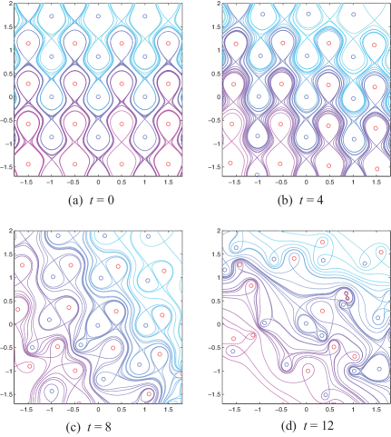
Figure 12: Snapshots of the streamlines plotted in a frame moving with the same velocity as the point vortex initially placed in the middle of the finite array of streets. This array includes 11 streets, each composed of 20 equal and opposite point vortices (yielding a total of 220 point vortices). The parameters that define the initial spacing of the vortices are set to $a=1$, $b=0.2805$, $h=0.861$ while the vortex strength is normalized to $\Gamma=1$. Clearly, the initial street-like configuration changes with time and eventually breaks completely.

6 Conclusions

The multiple wake system developed in this paper is proposed as a model of the mid-wake region generated by a school of fish, swimming in a coordinated fashion. Immediately behind each individual fish (i.e. the near-wake), a classical (reverse) von Kármán vortex street would be a standard model of the flow structure, whereas far downstream (i.e. the far-wake), viscous effects effectively diminish the presence of the entire wake from the school. However in the mid-wake region, the wake generated from each individual fish interacts nonlinearly with its neighbors to produce a complex structure whose streamline pattern depends on (i) the aspect ratio of each individual von Kármán vortex street, and (ii) the distance between neighboring streets. Our model shows that the closer the wakes are to their neighbors, the ‘wider’ the cooperative effect becomes, in the sense that more and more neighboring wakes are able to communicate and exchange fluid. The structures potentially affect the behavior of a fish swimming in this mid-wake region in two important ways. First, the separatrices produced by the field of wakes may effectively block passive locomotion of fish. There is however no guarantee that these separatrices which constitute barriers to passive tracers would also constitute barriers to passive locomotion of fish who, unlike passive tracers, may alter the streamline patterns in the flow (see for example [5]). Second, because of this ‘blocking’ effect, passive particles advected in the wake, such as nutrients, can be more effectively trapped, leading to benefits for the individual fish. The bifurcations of the streamline patterns were studied as a function of the wake parameters and shown to follow a geometric scaling law, not unlike the scaling law produced in a Fiegenbaum period-doubling cascade. Evolution patterns for finite-arrays show that the scaling laws and global streamline patterns discussed in the infinite array setting eventually break down and become more complex. However, for short times dictated by the aspect ratio of each street and the separation distance between the streets, near the center of the mid-wake regions, because the effect of the perturbations due to the finite-array has not yet been felt, the pattern from the infinite array prevails and is expected to play some determining role in the collective dynamics of the school. Future work will focus on whether these ‘cooperative’ features identified in this idealized setting persist in more realistic models which incorporate still more dynamical complexity such as the presence of moving boundaries that model the fish and in three-dimensions.

References

- [1] Abrikosov A.A. Nobel Lecture: Type-II superconductors and the vortex lattice. Rev. Mod. Phys., 76:975–979, 2004.
- [2] Aref H. [1995], On the equilibrium and stability of a row of point vortices, Journal of Fluid Mechanics, 290, 167-181.
- [3] Aref H., M. Bröns and M.A. Stremler [2007], Bifurcation and Instability Problems in Vortex Wakes. Journal of Physics: Conference Series - Second International Symposium on Instability and Bifurcations in Fluid Dynamics, IOP publishing 64 012015
- [4] Gelfreich, V.G. and V.F. Lazutkin [2001], Splitting of separatrices: perturbation theory and exponential smallness. Russian Mathematical Surveys, 56(3): 499-558.
- [5] Kanso, E., and B. Oskouei [2008], Stability of a Coupled Body-Vortex System, Journal of Fluid Mechanics, 800:77–94.
- [6] von Kármán, T. [1911], Über den mechanismus des widerstand den ein bewegter körper in einer üeig keit erfährt. Nachrichten der K. Gesellschaft der Wissenschaften zu Göttingen Math.-phys. Klasse pp. 1 9.
- [7] Knopp K. [1956], Infinite Sequences and Series, Dover publications, Inc., New York.
- [8] Kochin, N.E., I.A. Kibel, N.V. Roze [1964], Theoretical Hydrodynamics, Interscience Press.
- [9] Lamb, S. H. [1932], Hydrodynamics, Cambridge University Press.
- [10] Newton, P. K. [2001], The N-Vortex Problem Analytical Techniques, Springer.
- [11] O’Neil K. A. [1989], On the Hamiltonian Dynamics of vortex lattices, J Math. Phys. 30(6)1373-1379.
- [12] O’Neil, K. [2007], Continuous Parametric Families of Stationary and Translating Periodic Point Vortex Configurations, Journal of Fluid Mechanics, 591:393-441.
- [13] Rahaman Q., A. Alvarez-Toledo, B. Parker, and C. M. Ho [1988], Interaction of Two-Dimensional Wakes Physics of Fluids, 31(9), 2387.
- [14] Saffman, P. G. [1992], Vortex Dynamics, Cambridge University Press.
- [15] Saffman P.G. and J. Sheffield [1977], Flow over a wing with an attached free vortex, Studies in Applied Math., 57, 107-117.
- [16] Stremler, M. A. [2003], Relative Equilibria of Singly Periodic Point Vortex Arrays. Physics of Fluids Vol. 15 No. 12 3767-3775.
- [17] Stremler M. and H. Aref [1999], Motion of three point vortices in a periodic parallelogram, Journal of Fluid Mechanics, 392, 101-128.
- [18] Tkachenko, V.K. [1966], On vortex lattices, Soviet Phys. JETP, 22, 1282-1286.
- [19] Tkachenko, V.K. [1966], Stability of vortex lattices, Soviet Phys. JETP, 23, 1049-1056.
- [20] Weihs, D. [1973], Hydrodynamics of fish schooling, Nature, 241:290-291.
- [21] Weihs, D. [1975], Some hydrodynamical aspects of fish schooling, pp. 703–718. In T. Wu, C. J. Brokaw and C. Brennan (editors), Swimming and Flying in Nature, vol. 2, Plenum Press, New York.
- [22] Williamson, C.H.K. [1996], Vortex dynamics in the cylinder wake. Ann. Rev. Fluid Mech. 28, 477 539.