Infinite invariant densities for anomalous diffusion in optical lattices and other logarithmic potentials

Abstract

We solve the Fokker-Planck equation for Brownian motion in a logarithmic potential. When the diffusion constant is below a critical value the solution approaches a non-normalizable scaling state, reminiscent of an infinite invariant density. With this non-normalizable density we obtain the phase diagram of anomalous diffusion for this important process. We briefly discuss the consequence for a range of physical systems including atoms in optical lattices and charges in vicinity of long polyelectrolytes. Our work explains in what sense the infinite invariant density and not Boltzmann’s equilibrium describes the long time limit of these systems.

Brownian particles in contact with a thermal heat bath and in the presence of a binding potential field $V(x)$ attain a steady state which is the Boltzmann equilibrium distribution $W_{steady}(x)=N\exp[-V(x)/k_{b}T]$. An interesting case is the logarithmic potential: $V(x)\propto\epsilon_{0}\ln(x)$ for $x\gg 1$. Inserting $V(x)$ into the Boltzmann distribution, one finds that the steady state solution is described by an asymptotic power law $W_{steady}(x)\sim Nx^{-\epsilon_{0}/k_{b}T}$. $\epsilon_{0}/k_{b}T$ must be larger than one for the normalization $N$ to exist. Brownian motion in a logarithmic potential has attracted much attention since it describes many physical systems, ranging from diffusion of momentum of two level atoms in optical lattices CT ; Zoller ; Lutz , single particle models for long ranged interacting systems Bouchet ; Lemou , the famous problem of Manning condensation describing a charged particle in the vicinity of a long and uniformly charged wire (i.e. an ion in vicinity of a long charged polymer) Manning , and very recently the motion of nano-particles in an appropriately constructed force field Adam .

In this Letter we provide the long sought after CT ; Zoller ; Lutz ; Bouchet ; Lemou ; Chavanis long time solution of the Fokker-Planck equation describing the dynamics of Brownian particles in a logarithmic potential. Naively one would expect that in the long time limit the equilibrium distribution, i.e. the Boltzmann distribution, is reached; however the logarithmic potential turns out to be much more interesting. To start with, we point out that the second moment in the steady state $\langle x^{2}\rangle_{steady}$ may diverge, namely $\langle x^{2}\rangle_{steady}=\infty$ if $1<\epsilon_{0}/k_{b}T<3$. This behavior is unphysical. In particular in the context of optical lattices, it implies that the averaged kinetic energy of the atoms is infinite which is of course impossible (see details below). If we view the problem of Brownian diffusion in a logarithmic potential dynamically, we immediately realize that the process cannot be faster than diffusion; namely $\langle x^{2}\rangle\leq 2Dt$ where $D$ is the diffusion constant so $\langle x^{2}\rangle=\infty$ is wrong (we will soon derive this bound from the Fokker-Planck equation). In this sense the steady state solution, e.g. the Boltzmann distribution, for a particle in a logarithmic potential, does not describe the statistical properties of the problem, even in the limit of long times.

Here we show that Brownian particles in a logarithmic potential are characterized by an infinite invariant density. This density is not normalizable (hence the term infinite); however as we show, it does describe the anomalous behavior of the system. For example it can be used to obtain correctly the moments of the process, while the normalizable Boltzmann distribution completely fails to do so. We examine these issues first in the context of diffusion of momenta of atoms in an optical lattice, since this system is an excellent candidate to experimentally test our predictions in the lab. The reader should note that our results with some small notational changes describe a wide class of Brownian trajectories in the presence of a logarithmic potential (see discussion below).

Fokker-Planck equation. The equation for the probability density function (PDF) $W(p,t)$ of the momentum $p$ of an atom in an optical trap is modeled within the semi-classical approximation according to CT ; Zoller ; Lutz

$${\partial W\over\partial t}=D{\partial^{2}\over\partial p^{2}}W-{\partial\over\partial p}F(p)W.$$ (1)

The cooling force

$$F(p)=-{p\over 1+p^{2}}$$ (2)

restores the momentum to its minimum while $D$ describes stochastic momentum fluctuations which lead to heating. From the Sisyphus effect, interaction of atoms with the counter propagating laser beams means that $D$ is determined by the depth of the optical potential CT ; Zoller ; Lutz , which in turn leads to experimental control of the unusual statistical properties of this system Renzoni . For $p\ll 1$ the force is harmonic, $F(p)\sim-p$ while in the opposite limit, $p\gg 1$, $F(p)\sim-1/p$. The effective potential $V(p)=-\int^{p}F(p){\rm d}p=(1/2)\ln(1+p^{2})$ is symmetric $V(p)=V(-p)$ and $V(p)\sim\ln(p)$ when $p\gg 1$ (we use a dimensionless representation for $p$ Lutz ). The minima of the effective potential $V(p)$ is at $p=0$ which is of course the ideal cooling limit which is not maintained due to the fluctuations described here by $D$.

Steady state. The steady state solution of $W(p,t)$ is found in the usual way: imposing $\partial W_{steady}/\partial t=0$ from Eqs. (1,2) we have $W_{steady}\propto\exp[-V(p)/D]$. This solution is normalizable only if $D<1$ and for that case one finds the Tsallis distribution Lutz ; Renzoni

$$W_{steady}\left(p\right)={\cal N}\left(1+p^{2}\right)^{-1/(2D)}$$ (3)

where ${\cal N}=\Gamma\left({1\over 2D}\right)/[\sqrt{\pi}\Gamma\left({1-D\over 2D}\right)]$ is a normalization constant. This steady state solution was observed in optical lattice experiments Renzoni where it was shown that this behavior is tunable, namely one may control $D$ to obtain different steady state solutions. Notice that Eq. (3) exhibits a power law decay for large $p$ which is clearly related to the logarithmic potential under investigation. From Eq. (3) we have

$$\langle p^{2}\rangle_{steady}\sim\left\{\begin{array}[]{l l}{D\over 1-3D}&0<D<1/3\\ &\\ \infty&1/3<D<1.\end{array}\right.$$ (4)

As mentioned in the introduction the behavior $\langle p^{2}\rangle_{steady}=\infty$ is unphysical since it implies an averaged kinetic energy which is infinite Katori .

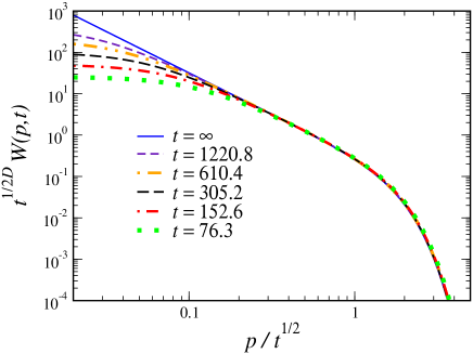
Figure 1: We show that $f(z)=t^{1/(2D)}W(p,t)$ $(z=p/t^{1/2})$ obtained from numerical solutions of the Fokker-Planck equation with a logarithmic potential, converges towards the infinite invariant density [solid blue $t=\infty$ curve Eq. (12)]. Thus the asymptotic behavior of the system is not globally determined by the standard steady state solution. Notice that for $t\to\infty$, $f(z)\sim z^{-1/D}$ for small $z$ and hence in in the long time limit the infinite invariant density $f(z)$ is non-normalizable. Here $D=1/2$ and initially $W(p,t=0)$ is a delta function centered on the origin.

Bounds on $\langle p^{2}\rangle$. To start our analysis we consider the dynamics of $\langle p^{2}\rangle$. Multiplying the Fokker-Planck Eq. (1) with $p^{2}$ and integrating over $p$ we have, after integrating by parts and using the natural boundary condition that $W(p,t)$ and its derivative at $p\to\pm\infty$ are zero,

$${\partial\over\partial t}\langle p^{2}\rangle=2D-2\langle{p^{2}\over 1+p^{2}}\rangle$$ (5)

where $\langle...\rangle=\int_{-\infty}^{\infty}...W(p,t){\rm d}p$. Obviously we have

$$0\leq\langle{p^{2}\over 1+p^{2}}\rangle\leq 1,$$ (6)

hence $2D-2\leq{\partial\langle p^{2}\rangle\over\partial t}\leq 2D$, and therefore if we start with a finite $\langle p^{2}\rangle$ we have in the long time limit

$$(2D-2)t\leq\langle p^{2}\rangle\leq 2Dt.$$ (7)

The upper bound clearly implies that $\langle p^{2}\rangle$ increases at most linearly as diffusion persists. The lower bound is useful when $D>1$ since then it shows that $\langle p^{2}\rangle\propto t$. We call the case $D>1$ the diffusive regime. We now turn to analyze the cases $D>1$ and $D<1$ separately since they exhibit very different behaviors.

The case $D<1$. We now consider the more interesting case $D<1$ where a normalizable steady state Eq. (3) exists. In the long time limit the latter describes well the central part of $W(p,t)$ but not its tails which govern the growth of $\langle p^{2}\rangle$ when $1/3<D<1$ (for $D<1/3$ higher order moments diverge and the essential problem remains). We employ the scaling ansatz remarkf

$$W(p,t)\sim t^{\alpha}f(p/\sqrt{t})$$ (8)

which holds for large $p$ and long $t$ and the exponent $\alpha$ will be soon determined. Let us introduce the scaling variable $z=p/t^{1/2}$. This is the typical scaling of Brownian motion, which indicates that for large $p$ diffusion is in control; however as we now show, $f(z)$ in far from a Gaussian so the process is clearly not simple diffusion. Inserting Eq. (8) in the Fokker-Planck equation (1) and using $p\gg 1$ we find

$$D{d^{2}f\over dz^{2}}+\left({1\over z}+{z\over 2}\right){df\over dz}-\left(\alpha+{1\over z^{2}}\right)f=0.$$ (9)

For small $z$ we get $f\sim z^{-1/D}$ or $f\sim z$; the latter is rejected since $f(z)$ cannot increase with $z$. To find $\alpha$ we require that the small $z$ solution matches the steady state, since the latter describes well the density in the center. Using Eq. (8) with $f\propto z^{-1/D}$ we have $W(p,t)\propto t^{\alpha+1/(2D)}p^{-1/D}$ which is to be matched with the steady state solution Eq. (3) $W_{steady}\propto p^{-1/D}$. Hence we have

$$\alpha=-{1\over 2D}.$$ (10)

In this case one solution of Eq. (9) is immediate: $f(z)=Az^{-1/D}$. While this solution has the correct small $z$ behavior it does not decay quickly enough at large $z$ remark0 , so we need the second solution. The later is found by the method of reduction of order:

$$f(z)=Az^{-1/D}\int_{z}^{\infty}s^{1/D}e^{-s^{2}/4D}{\rm d}s.$$ (11)

The constant $A$ is found by matching the small $z$ solution Eq. (11) to the steady state solution Eq. (3). Solving the integral in Eq. (11) we reach our first main result

$$f(z)={{\cal N}z^{-1/D}\over\Gamma\left({1+D\over 2D}\right)}\Gamma\left({1+D\over 2D},{z^{2}\over 4D}\right)$$ (12)

where $\Gamma(a,x)=\int_{x}^{\infty}e^{-s}s^{a-1}{\rm d}s$ is the incomplete Gamma function Abr and $\Gamma(a)$ is the Gamma function. For small and large $z$ we find

$$f(z)\sim\left\{\begin{array}[]{l l}{\cal N}z^{-1/D}&\ \ z\ll 2\sqrt{D}\\ {{\cal N}\left(4D\right)^{{1\over 2}-{1\over 2D}}\over\Gamma\left({1+D\over 2D}\right)}z^{-1}e^{-z^{2}/4D}&\ \ z\gg 2\sqrt{D}.\end{array}\right.$$ (13)

Eq. (12) is non-normalizable since according to Eq. (13) $f(z)\sim z^{-1/D}$ and hence $\int_{0}^{\infty}f(z){\rm d}z=\infty$.

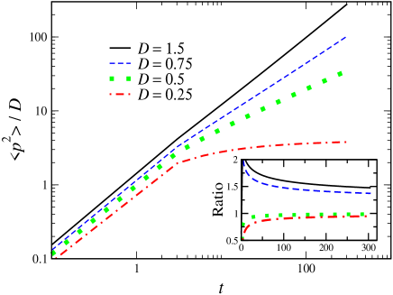
Figure 2: In the long time limit the variance $\langle p^{2}\rangle$ exhibits three behaviors: normal diffusion if $D>1$, anomalous diffusion $\langle p^{2}\rangle\sim t^{3/2-1/(2D)}$ if $1/3<D<1$ and steady state behavior $\langle p^{2}\rangle\to\mbox{const}$ for $D<1/3$. For very short times (not shown) $\langle p^{2}\rangle\sim 2Dt$ since then the influence of the force field is negligible (initially particles are on the origin). In the inset we show that the ratio of $\langle p^{2}\rangle$ obtained from simulations to $\langle p^{2}\rangle$ found from the asymptotic formula Eq. (17) approaches unity as time increases.

Infinite invariant density. We call the non-normalizable solution Eq. (12) an infinite invariant density. In Fig. 1 comparison is made between our analytical solution Eq. (12) and numerical solutions of the Fokker-Planck equation. As time increases, the solution in the scaled coordinate approaches the infinite invariant density Eq. (12), which describes the asymptotic scaling solution of the probability density. For any finite long time $t$, expected deviations from the infinite invariant solution are found for small values of $z$ (see Fig. 1). These deviations become negligible at $t\to\infty$ however they are important since they indicate that the pathological divergence of $f(z)$ on the origin is slowly approached but never actually reached, namely the solution is of course normalizable for finite measurement times.

The variance $\langle p^{2}\rangle$. Even though the solution Eq. (12) is non-normalizable, it can be used to find the second moment $\langle p^{2}\rangle$. To see this we introduce a cutoff $p_{c}$ above which our solution Eq. (12) is valid. The variance is calculated in the usual way exploiting symmetry $W(p,t)=W(-p,t)$

$$\langle p^{2}\rangle=2\int_{0}^{p_{c}}p^{2}W(p,t){\rm d}p+2\int_{p_{c}}^{\infty}p^{2}W(p,t){\rm d}p.$$ (14)

The first term in Eq. (14) is a constant and can be neglected once the second term is shown to increase with time. Inserting the infinite invariant solution Eq. (12) in the second term of Eq. (14)

$$\langle p^{2}\rangle\sim 2t^{{3\over 2}-{1\over 2D}}\int_{p_{c}/\sqrt{t}}^{\infty}z^{2}f(z){\rm d}z$$ (15)

for $1/3<D<1$. The lower limit in the integral $p_{c}/t^{1/2}$ goes to zero when $t\to\infty$ and the diffusion is anomalous

$$\langle p^{2}\rangle\sim 2t^{{3\over 2}-{1\over 2D}}\int_{0}^{\infty}z^{2}f(z){\rm d}z.$$ (16)

Thus the infinite invariant density yields the anomalous diffusion in this model. While $f(z)\sim z^{-1/D}$ for small $z$ and is hence non-normalizable, the integral in Eq. (16) is finite: the $z^{2}$ cures the pathology of the density at the origin. Solving the integral in Eq. (16) as well as the diffusive regime soon to be discussed we obtain

$$\langle p^{2}\rangle\sim\left\{\begin{array}[]{l l}{D\over 1-3D}&D<{1\over 3}\\ &\\ {16{\cal N}\over 2^{1/D}\Gamma\left({1+D\over 2D}\right)}{D\over 3D-1}\left(Dt\right)^{{3\over 2}-{1\over 2D}}&{1\over 3}<D<1\\ &\\ 2\left(D-1\right)t&1<D.\end{array}\right.$$ (17)

For $D<1/3$, $\langle p^{2}\rangle$ is time independent and is determined by the steady state solution Eq. (3). For the intermediate regime $1/3<D<1$ the diffusion is anomalous, while for $D$ larger than $1$ it is normal in agreement with the simple bounds we have found, Eq. (7). In Fig. 2, numerical solutions for $\langle p^{2}\rangle$ versus time exhibit convergence towards these types of behavior.

A simple argument for the anomalous diffusion exponent in Eq. (17), for $1/3<D<1$, is found by noticing that the steady state solution Eq. (3) describes the center part of the PDF however with cutoffs determined by diffusion (i.e. $|p|<\sqrt{Dt}$) hence

$$\langle p^{2}\rangle\propto\int^{\sqrt{Dt}}_{-\sqrt{Dt}}p^{2}W_{steady}(p){\rm d}p\propto 2\int^{\sqrt{t}}p^{2-{1/D}}{\rm d}p\propto t^{{3\over 2}-{1\over 2D}}.$$ (18)

To characterize the distribution of $p$ and to find $\langle p^{2}\rangle$ exactly, we need the infinite invariant density which cannot be obtained by similar simple scaling arguments.

The case $D>1$. We now investigate the diffusive regime $D>1$ where the steady state solution is non-normalizable. In this case our bound Eq. (7) yields diffusive behavior $p\propto\sqrt{t}$ which suggests a scaling solution $W(p,t)=t^{\alpha}f(z)$ where now $\alpha=-1/2$ and as before $z=p/\sqrt{t}$ remarkf . Eq. (9) is still valid and its solution when $\alpha=-1/2$ is

$$f(z)={z^{-1/D}e^{-z^{2}\over 4D}\over\left(4D\right)^{1-\beta}\Gamma\left(1-\beta\right)}$$ (19)

where $\beta=(1+D)/(2D)$. Notice that when $D\gg 1$ we have $f(z)\sim\exp(-z^{2}/4D)/\sqrt{4\pi Dt}$ which is expected from a purely Gaussian diffusive process. Roughly speaking the potential is responsible for accumulating of particles close to the origin which yields the $z^{-1/D}$ factor in Eq. (19). Similar to the case $D<1$ the solution Eq. (19) exhibits a divergence on $z=0$ since $f(z)\sim z^{-1/D}$. However, since now $D>1$ the solution is normalizable and in this regime we do not find an infinite invariant density. Finally with Eq. (19) we obtain $\langle p^{2}\rangle$ for $D>1$ which was given in Eq. (17).

The role of infinite invariant density in physics is now briefly discussed. Mathematicians have investigated infinite invariant measures in the context of ergodic theory for many years Aaronson . More recently, an infinite invariant density Korabel was shown to describe weak chaos in the well known intermittent Pomeau-Manneville map (by weak chaos we mean dynamical systems with zero Lyapunov exponent which still exhibit stochastic behavior). In the context of a model of an electron glass, the distribution of eigenvalues of a relaxation matrix were found to be non-normalizable which yields slow relaxations and aging Amir . Thus three routes to infinite invariant densities are: weak chaos, disorder and as we showed here the widely applicable case of diffusion in a logarithmic potential. These vastly different mechanisms all exhibit anomalous diffusion and the usual ergodic hypothesis breaks down. It therefore seems likely and certainly worthy of further investigation that a broad range of physical systems which exhibit anomalous kinetics Bouchaud ; Review ; Levybook are described by an infinite invariant densities.

Thermal systems. So far we have used the example of the motion of two level atoms in an optical lattice, a system which is not thermal and its equilibrium distribution is strictly speaking not a Boltzmann equilibrium. As noted in the introduction we may consider over-damped Brownian particles coupled to a thermal heat bath with temperature $T$ and get the same results. More precisely consider over-damped Brownian motion in the potential $\epsilon_{0}\ln\left(a^{2}+x^{2}\right)/2$ and diffusion constant $\overline{D}$ (units $m^{2}/s$). With the fluctuation dissipation theorem Risken we have

$${\partial P(\tilde{x},\tilde{t})\over\partial\tilde{t}}={k_{b}T\over\epsilon_{0}}{\partial^{2}\over\partial\tilde{x}^{2}}+{\partial\over\partial\tilde{x}}{\tilde{x}\over 1+\tilde{x}^{2}}P\left(x,t\right)$$ (20)

which after obvious change of notation is the same as Eq. (1). In Eq. (20) dimensionless time $\tilde{t}=\epsilon_{0}\overline{D}t/a^{2}k_{b}T$ and space $\tilde{x}=x/a$ are used. More importantly our results are not limited to one dimension. Indeed an infinite wire of radius $a$, with uniform charge density per unit length $\lambda$ yields the logarithmic potential $V(r)=\lambda ln(r)$ for $r>a$ and $a>0$ must be finite. Such a potential was considered by Manning Manning in the context of ion condensation on a long polyelectrolyte. Using cylindrical coordinates it is not difficult to show that the corresponding three dimensional Fokker Planck equation maps onto a one dimension problem (for coordinate $r$) which is similar to ours. We do note that the limit $a\to 0$ yields new behaviors beyond what we discussed here (this is related to the fact that our potential is finite on $p=0$ while $ln(r)\to-\infty$ for $r\to 0$, i.e. when $a$ approaches zero).

Summary. Steady state solutions are commonly assumed to describe the long time limit of dynamics of many thermal and non-thermal systems. This assumption is one of the pillars on which statistical mechanics is built. Therefore it was rewarding to find that for the widely applicable process of Brownian motion in a logarithmic potential, an infinite invariant density describes the scaling solution. Both the well known steady state solution Eq. (3) and the infinite invariant density Eq. (12) found here are needed to characterize the long time solution. Thus Boltzmann’s equilibrium concepts while important are clearly not sufficient.

Acknowledgment Work is supported by the Israel Science Foundation. EB thanks E. Lutz and F. Renzoni for useful discussion on the physics of optical lattices.

References

- (1) Y. Castin, J. Dalibard, and C. Cohen-Tannoudji, in Light Induced Kinetic Effects on Atoms, Ions and Molecules, edited by L. Moi et al. (ETS Editrice, Pisa, 1991).
- (2) S. Marksteiner, K. Ellinger, and P. Zoller, Phys. Rev. A 53 3409 (1996).
- (3) E. Lutz, Phys. Rev. Lett. 93 190602 (2004).
- (4) F. Bouchet, and T. Dauxois, Physical Review E 72 045103(R) (2005). ibid Journal of Physics: Conference Series 7 34 (2005)
- (5) P.H. Chavanis, and M. Lemou, Eur. Phys. J. B 59 217-247 (2007).
- (6) G. S. Manning, J. of Chemical Physics 51 924 (1969).
- (7) A. E. Cohen Phys. Rev. Lett. 94 118102 (2005)
- (8) P. H. Chavanis, and M. Lemou Phys. Rev. E 72, 061106 (2005).
- (9) P. Douglas, S. Bergamini, and F. Renzoni, Phys. Rev. Lett. 96 110601 (2006).
- (10) H. Katori, S. Schlipf, and H. Walther, Phys. Rev. Lett. 79 2221 (1997) found the finger print of this divergence as a dramatic increase of energy when the depth of the optical potential was carefully tuned.
- (11) This scaling ansatz can be derived from the formal solution of the Fokker-Planck equation (in preparation).
- (12) If we have which is too slow a decay to describe the process with initial condition centered in the vicinity of the origin. In fact yields for while we proved so the solution is rejected. An obvious exception is the case were we start the process in the steady state, then one may get for all time which is valid mathematically but physically wrong.
- (13) M. Abramowitz, and I. A. Stegun, Handbook of Mathematical Functions Dover (New York) 1972.
- (14) J. Aaronson, An Introduction to Infinite Ergodic Theory American Mathematical Society (1997).
- (15) N. Korabel, and E. Barkai, Phys. Rev. Lett. 102, 050601 (2009).
- (16) A. Amir, Y. Oreg, and Y. Imry Phys. Rev. Lett. 103 126403 (2009).
- (17) J. P. Bouchaud, and A. Georges, Phys. Rep. 195, 127 (1990).
- (18) R. Metzler, J. Klafter, Phys. Rep. 339, 1 (2000).
- (19) F. Bardou, J. P. Bouchaud, A. Aspect, and C. Cohen-Tannoudji Lévy Statistics and Laser Cooling Cambridge University Press (2002)
- (20) H. Risken The Fokker-Planck Equation Springer (Berlin) (1996).