A microscopic mechanism for increasing
thermoelectric efficiency

Abstract

We study the coupled particle and energy transport in a prototype model of interacting one-dimensional system: the disordered hard-point gas, for which numerical data suggest that the thermoelectric figure of merit $ZT$ diverges with the system size. This result is explained in terms of a microscopic mechanism, namely the local equilibrium is characterized by the emergence of a broad stationary “modified Maxwell-Boltzmann velocity distribution”, of width much larger than the mean velocity of the particle flow.

1 Introduction

Thermoelectricity is an old field: The Seebeck effect, that is, the conversion of temperature differences into electricity, was discovered in 1821. However, a strong interest in termoelectric phenomena arose only in the 1950’s, when Ioffe discovered that doped semiconductors exhibited much larger thermoelectric effect than did other materials. He also proposed that semiconductors could be used to build solid-state home refrigerators. Such refrigerators would be long-lived, silent, maintenace-free, and environmentally benign. Ioffe’s suggestion initiated an intense research activity in semiconductors physics [1, 2, 3]. However, in spite of all efforts and consideration of all type of semiconductors, thermoelectric refrigerators have still poor efficiencies compared to compressor-based refrigerators. Today, thermoelectric devices are mainly used in situations in which reliability and quiet operation are more important than the cost. Applications include equipments in medical applications, space probes, etc.

In the last decade there has been an increasing pressure to find better thermoelectric materials with higher efficiency. The reason is the strong environmental concern about chlorofluorocarbons used in most compressor-based refrigerators. Also the possibility to generate electric power from waste heat using thermoelectric effect is becoming more and more interesting [1, 2, 3, 4].

The thermodynamic efficiency can be conveniently written in terms of the so-called figure of merit $ZT=(\sigma S^{2}/\kappa)T$, where $\sigma$ is the electric conductivity, $S$ the thermoelectric power (Seebeck coefficient), $\kappa$ the thermal conductivity, and $T$ the temperature. Ideal Carnot efficiency is recovered in the limit $ZT\to\infty$. In spite of the worldwide research efforts for identifying thermoelectric materials with high $ZT$ values, so far the best thermoelectric materials are characterized by values of $ZT\sim 1$, at room temperature. Values $ZT>3$ are considered to be essential for thermoelectric devices to compete in efficiency with mechanical power generation and refrigeration.

The challenge lies in engineering a material for which the values of $\sigma$, $S$, and $\kappa$ can be controlled in order to optimize thermoelectric efficiency. The problem is that the different transport coefficients are interdependent, thus making optimization extremely difficult. On the other hand, thermodynamics does not impose any upper bound on $ZT$, so that efficient thermoelectric devices could in principle be engineered. The present understanding of the possible microscopic mechanisms leading to an increase of $ZT$ is quite limited, with few exceptions. Notably, Refs. [5, 6] showed that the optimal density of states in a thermoelectric material is a delta function. Such sharp energy filtering allows to reach, in principle, the Carnot efficiency.

Here we consider the problem of increasing thermoelectric efficiency from a new perspective, that is, we pursue a dynamical system approach. Understanding from first principles and from nonlinear dynamics simulations the microscopic mechanisms that can be implemented to control the heat flow [7] might prove useful not only for thermoelectric phenomena but also for the design and engineering of thermal diodes and transistors. In this paper, our plan is to compute transport coefficients and thermoelectric efficiency from first principles, namely from the underlying microscopic dynamical processes which are known to be predominantly nonlinear in nature. In a previous work [8], the thermoelectric problem has been investigated by numerical solution of the microscopic equations of motion. Inspired by the kinetic theory of ergodic gases and chaotic billiards, a simple microscopic mechanism for increasing thermoelectric efficiency was proposed. More precisely, the cross transport of particles and energy in open classical ergodic billiards was considered. It has been shown that, in the linear response regime, the thermoelectric efficiency can approach Carnot efficiency for sufficiently complex charge carrier molecules. Indeed, the figure of merit has been found to be a growing function of the number $d_{\rm int}$ of internal degrees of freedom, $ZT=(d+1+d_{\rm int})/2$, where $d$ is the geometric dimension.

In spite of the abstract nature of the model, the above paper opens the possibility for a theoretical understanding of the basic microscopic requirements that a classical dynamical system must fulfill in order to lead to a high thermoelectric figure of merit. In particular, the question arises whether inter-particle interaction might increase the effective number of degrees of freedom, thus leading to a higher figure of merit than in the noninteracting idealized $d$ dimensional gas, where $ZT=(d+1)/2$. Alnog these lines a detailed numerical study of the cross heat and particle transport has been performed for an open one-dimensional disordered hard-point gas [9]. It has been found that $ZT$ diverges as a power-law in thermodynamic limit, $ZT\propto N^{b}$, where $N$ is the average number of particles in the system and $b\approx 0.79$. Even though the above result could be, in principle, very interesting, no indication was given concerning the microscopic mechanism which is responsible for the increase of $ZT$. On the other hand a theoretical understanding is needed in order to obtain useful hints for increasing thermodynamic efficiency in more realistic models.

In this paper, we propose a mechanism which explains the large thermoelectric quality factor $ZT$ numerically observed in Ref. [9]. This mechanism requires local equilibrium, as naturally expected in systems with the mixing property, and the emergence, in the linear response regime, of an out-of-equilibrium “modified Maxwell-Boltzmann velocity distribution” of width much larger than the mean velocity of the particle flow. Such broad distribution limit is opposite to the limit of peaked distribution, corresponding to the delta-like energy filtering put forward in Refs. [5, 6]. We provide numerical evidence supporting the effectiveness of the broad-distribution mechanism in the hard-point gas model.

Our paper is organized as follows. Secs. 2, 3, and 4 review introductory material on coupled particle and energy transport, modeling stochastic baths, and thermoelectric efficiency of the one-dimensional ideal non-interacting gas. In Sec. 5, we present numerical results for thermodynamic transport coefficients for the disordered hard-point gas model. Finally, the obtained numerical results are explained in terms of a mechanism based on the emergence of a broad stationary out-of-equilibrium velocity distribution. Concluding remarks are drawn in Sec. 6.

2 The thermoelectric figure of merit $ZT$

Let us focus our attention on a conductor in which both electric and heat current flow in one dimension (say, parallel to the $x$-direction). Assuming local equilibrium, a local entropy (per unit volume) $s$ can be defined, and the rate of entropy production reads [10]

$$\dot{s}=J_{u}\partial_{x}\left(\frac{1}{T}\right)+J_{\rho}\partial_{x}\left(-\frac{\mu}{T}\right),$$ (1)

in which $J_{u}$ and $J_{\rho}$ are the energy and particle current densities (fluxes) and $\partial_{x}(1/T)$, $-\partial_{x}(\mu/T)$ the associated generalized forces (affinities), where $T$ is the temperature and $\mu$ the electrochemical potential.

Assuming that the generalized forces are small, the relationship between fluxes and forces is linear and described by the phenomenological non equilibrium thermodynamic kinetic equations [10, 11]

$$J_{u}=L_{uu}\partial_{x}\left(\frac{1}{T}\right)+L_{u\rho}\partial_{x}\left(-\frac{\mu}{T}\right),$$ (2)

$$J_{\rho}=L_{\rho u}\partial_{x}\left(\frac{1}{T}\right)+L_{\rho\rho}\partial_{x}\left(-\frac{\mu}{T}\right),$$ (3)

with $L_{\alpha,\beta}$ ($\alpha,\beta\in\{u,\rho\}$) Onsager coefficients. In the absence of magnetic fields, due to microscopic reversibility of the dynamics, the Onsager reciprocity relation $L_{u\rho}=L_{\rho u}$ holds.

In analogy with the relation $dQ=TdS$, the heat current density $J_{q}$ can be defined by the relation

$$J_{q}=TJ_{s},$$ (4)

with

$$J_{s}=\frac{1}{T}J_{u}-\frac{\mu}{T}J_{\rho}$$ (5)

current density of entropy, and therefore

$$J_{q}=J_{u}-\mu J_{\rho}.$$ (6)

The entropy production rate equation can then be written in terms of the fluxes $J_{q}$ and $J_{\rho}$ and of the corresponding generalized forces $\partial_{x}(1/T)$ and $-(1/T)\partial_{x}\mu$:

$$\dot{s}=J_{q}\partial_{x}\left(\frac{1}{T}\right)+J_{\rho}\left(-\frac{\partial_{x}\mu}{T}\right),$$ (7)

while the linear relationship between fluxes and forces reads as follows:

$$J_{q}=\tilde{L}_{qq}\partial_{x}\left(\frac{1}{T}\right)+\tilde{L}_{q\rho}\left(-\frac{\partial_{x}\mu}{T}\right),$$ (8)

$$J_{\rho}=\tilde{L}_{\rho q}\partial_{x}\left(\frac{1}{T}\right)+\tilde{L}_{\rho\rho}\left(-\frac{\partial_{x}\mu}{T}\right),$$ (9)

with $\tilde{L}_{\rho\rho}=L_{\rho\rho}$, $\tilde{L}_{q\rho}=\tilde{L}_{\rho q}$ (Onsager relation), $\tilde{L}_{q\rho}=L_{u\rho}-\mu L_{\rho\rho}$, $\tilde{L}_{qq}=L_{uu}-2\mu L_{u\rho}+\mu^{2}L_{\rho\rho}$. Note that, if we call ${\bf L}$ and ${\bf\tilde{L}}$ the $2\times 2$ Onsager matrices with matrix elements $L_{\alpha\beta}$ ($\alpha,\beta\in\{u,\rho\}$) and $\tilde{L}_{\gamma\delta}$ ($\gamma,\delta\in\{q,\rho\}$), it turns out that ${\det}{\bf\tilde{L}}={\det}{\bf L}$.

The Onsager coefficients can be expressed in terms of more familiar quantities, the electric conductivity $\sigma$, the thermal conductivity $\kappa$, and the Seebeck coefficient (thermopower) $S$. Let us first consider the case in which the thermal gradient vanishes, $\partial_{x}T=0$, and the system is homogeneous, so that the chemical potential $\mu_{c}$ is uniform. Since the electrochemical potential $\mu$ is composed of a chemical part $\mu_{c}$ and an electric part $\mu_{e}$, $\mu=\mu_{c}+\mu_{e}$, it turns out that for a homogeneous isothermal system $\partial_{x}\mu=\partial_{x}\mu_{e}$. The electric current $J_{e}=eJ_{\rho}$, with $e$ charge of the conducting particles, is then given by $J_{e}=\sigma\mathcal{E}=-(\sigma/e)\partial_{x}\mu_{e}$, with $\mathcal{E}$ external electric field applied to the system. The quantities $\mu_{c}$ and $\mu_{e}$ cannot be determined separately by the theory of irreversible thermodynamics [12]: only their combination $\mu=\mu_{c}+\mu_{e}$ appears in the kinetic equations (2) and (3). Based on this equivalence, we can write $J_{\rho}=J_{e}/e=-(\sigma/e^{2})\partial_{x}\mu$ even when $\mu_{c}\neq 0$, provided $\partial_{x}T=0$, whence Eq. (9) gives

$$\sigma=\frac{e^{2}}{T}\tilde{L}_{\rho\rho}=\frac{e^{2}}{T}L_{\rho\rho}.$$ (10)

The heat conductivity $\kappa$ is defined as the heat current density per unit temperature gradient for zero electric current: $J_{q}=-\kappa\partial_{x}T$, at $J_{e}=0$. Solving the two kinetic equations (8) and (9) simultaneously, we obtain

$$\kappa=\frac{1}{T^{2}}\frac{\det\tilde{\bf L}}{\tilde{L}_{\rho\rho}}=\frac{1}{T^{2}}\frac{\det{\bf L}}{{L}_{\rho\rho}}.$$ (11)

Finally, the Seebeck coefficient $S$ is defined as the change in electrochemical potential per unit charge, $-\partial_{x}\mu/e$, per unit change in temperature difference: $S=-(1/e)\partial_{x}\mu/\partial_{x}T$, at $J_{e}=0$. We then obtain from Eq. (9)

$$S=\frac{\tilde{L}_{q\rho}}{eT\tilde{L}_{\rho\rho}}=\frac{1}{eT}\left(\frac{L_{u\rho}}{L_{\rho\rho}}-\mu\right).$$ (12)

It is of course possible to eliminate the three Onsager coefficients $\tilde{L}_{qq}$, $\tilde{L}_{q\rho}$, and $\tilde{L}_{\rho\rho}$ from the kinetic equations (8) and (9), and rewrite such equations is terms of the conductivities $\sigma$ and $\kappa$, and of the thermopower $S$:

$$J_{q}=-(\kappa+T\sigma S^{2})\partial_{x}T-\frac{T\sigma S}{e}\partial_{x}\mu,$$ (13)

$$J_{\rho}=-\frac{\sigma}{e^{2}}\partial_{x}\mu-\frac{\sigma S}{e}\partial_{x}T.$$ (14)

By eliminating $\partial_{x}\mu$ from the above two equations one can express $J_{q}$ in terms of $J_{\rho}$ and $\partial_{x}T$. It is then easy to derive an interesting expression for the entropy current density $J_{s}=J_{q}/T$ [10]:

$$J_{s}=eSJ_{\rho}-\frac{\kappa}{T}\partial_{x}T,$$ (15)

from which the Seebeck coefficient can be understood as the entropy transported (per unit charge) by the electron flow. The second contribution to the entropy flow, namely the term $-(\kappa/T)\partial_{x}T$, is independent of the particle current.

The thermoelectric efficiency $\eta$, of converting the input heat into output work, is determined by the non-dimensional figure of merit

$$ZT\equiv\frac{\sigma S^{2}}{\kappa}T.$$ (16)

To derive the relation between $\eta$ and $ZT$, we consider a one-dimensional system whose left/right ends are connected with left/right thermochemical reservoirs, with small temperature difference $\Delta T\equiv T_{R}-T_{L}$ and electrochemical potential difference $\Delta\mu\equiv\mu_{R}-\mu_{L}$. The efficiency $\eta$ is given, under steady state conditions, by the ratio of the time derivatives of the extracted work over the heat leaving the hot reservoir:

$$\eta=\frac{\dot{W}}{\dot{Q}}=\frac{\Delta\mu J_{\rho}}{J_{q}}.$$ (17)

Using Eqs. (13) and (14) to eliminate $\partial_{x}\mu$ and $J_{q}$, we obtain

$$\eta=\eta_{C}\,\frac{T}{\sigma\partial_{x}T}\,\frac{J_{e}^{2}+\sigma S\partial_{x}TJ_{e}}{TSJ_{e}-k\partial_{x}T},$$ (18)

where $\eta_{C}=1-T_{R}/T_{L}$ is the Carnot efficiency (here we assume $T_{L}>T_{R}$). The maximum efficiency for a given $\Delta T$ is derived after optimizing (18) with respect to $J_{e}$:

$$\eta_{\rm max}=\eta_{C}\frac{\sqrt{ZT+1}-1}{\sqrt{ZT+1}+1}.$$ (19)

The Carnot efficiency is therefore achieved in the limt $ZT\to\infty$.

Using Eqs. (10), (11), and (12), we can express $ZT$ in terms of the Onsager coefficients:

$$ZT=\frac{\tilde{L}_{q\rho}^{2}}{\det{\bf\tilde{L}}}=\frac{(L_{u\rho}-\mu L_{\rho\rho})^{2}}{\det{\bf L}}.$$ (20)

The only thermodynamic restrictions to the Onsager coefficients come from the positivity of the entropy production, $\dot{s}\geq 0$, which is a quadratic form in the generalized forces $\partial_{x}(1/T)$ and $-\partial_{x}(\mu/T)$ (see Eqs. (1)-(3)) or $\partial_{x}(1/T)$ and $-(1/T)\partial_{x}\mu$ (see Eqs. (7)-(9)). Condition $\dot{s}\geq 0$ implies $L_{uu},L_{\rho\rho}\geq 0$, $\det{\bf L}\geq 0$ in the first case, $\tilde{L}_{qq},\tilde{L}_{\rho\rho}\geq 0$, $\det{\bf\tilde{L}}\geq 0$ in the latter. Thus, the only restriction to the thermoelectric figure of merit is $ZT\geq 0$, so that in principle Carnot efficiency can be achieved.

It is clear from Eq. (20) that $ZT$ diverges iff the Onsager matrix ${\bf L}$ (or, equivalently, ${\bf\tilde{L}}$) is ill-conditioned, that is, when the condition number $\lambda_{1}({\bf L})/\lambda_{2}({\bf L})$ diverges, where $\lambda_{1}({\bf L})$ and $\lambda_{2}({\bf L})$ are the largest and the smallest eigenvalue of ${\bf L}$, respectively. The condition number diverges iff the quantity

$${\rm cond}({\bf L})\equiv\frac{[{\rm Tr}({\bf L})]^{2}}{\det({\bf L})}$$ (21)

diverges. In this case the system (2)-(3) (or, equivalently, the system (8)-(9)) becomes singular, and therefore $J_{u}\propto J_{\rho}$. In short, the Carnot efficiency is obtained iff the energy and particle currents are proportional.

3 Modeling thermochemical baths

We consider a one-dimensional system whose ends are in contact with left/right baths (reservoirs), which are able to exchange energy and particles with the system, at fixed temperature $T_{\alpha}$ and electrochemical potential $\mu_{\alpha}$, where $\alpha=L,R$ denotes the left/right bath.

The thermochemical reservoirs are modeled as infinite one-dimensional ideal gases. Therefore, particle velocities in the reservoirs are described by the Maxwell-Boltzmann distribution,

$$f_{\alpha}(v)=\sqrt{\frac{m}{2\pi k_{B}T_{\alpha}}}\exp\left(-\frac{mv^{2}}{2k_{B}T_{\alpha}}\right),$$ (22)

where $k_{B}$ is the Boltzmann constant and $m$ the mass of the particles. We use a stochastic model of the thermochemical baths [13]: Whenever a particle of the system crosses the boundary which separates the system from the left or right reservoir, it is removed. On the other hand, particles are injected into the system from the boundaries, with rates $\gamma_{\alpha}$. The injection rate $\gamma_{\alpha}$ is computed by counting how many particle from reservoir $\alpha$ cross the reservoir-system boundary per unit time. That is to say,

$$\gamma_{\alpha}=\rho_{\alpha}\int_{0}^{\infty}dvvf_{\alpha}(v)=\rho_{\alpha}\sqrt{\frac{k_{B}T_{\alpha}}{2\pi m}},$$ (23)

with $\rho_{\alpha}$ density of the ideal gas in reservoir $\alpha$. Therefore, particles are injected into the system with velocity distribution

$$P_{\alpha}(v)=\frac{m}{k_{B}T_{\alpha}}\,v\exp\left(-\frac{mv^{2}}{2k_{B}T_{\alpha}}\right)\theta_{\alpha}(v),$$ (24)

where $\theta_{\alpha}(v)$ are step functions: $\theta_{L}(v)=1$ if $v\geq 0$, 0 otherwise; $\theta_{R}(v)=1$ if $v\leq 0$, 0 otherwise. We assume that injections from a macroscopic reservoir are independent events and that the time interval between subsequent injections satisfies the Poissonian distribution,

$${\cal P}_{\alpha}(t)=\gamma_{\alpha}\exp(-\gamma_{\alpha}t),$$ (25)

so that the average time between injections is $1/\gamma_{\alpha}$.

In order to relate the density $\rho_{\alpha}$ to the electrochemical potential $\mu_{\alpha}$, it is convenient to write the grand partition function

$$\Xi_{\alpha}=\sum_{N=0}^{\infty}\frac{1}{N!}\left\{\frac{\Lambda}{h}e^{\beta_{\alpha}\mu_{\alpha}}\int dv\,m\exp\left[-\beta_{\alpha}\left(\frac{1}{2}mv^{2}\right)\right]\right\}^{N},$$ (26)

with ${\Lambda}$ and $N$ size and number of particles of the reservoir, respectively , $\beta_{\alpha}\equiv 1/(k_{B}T_{\alpha})$ and $h$ the Planck’s constant. We then compute the average number of particles as

$$\langle N\rangle_{\alpha}=\frac{1}{\beta_{\alpha}}\frac{\partial}{\partial\mu_{\alpha}}\ln\Xi_{\alpha},$$ (27)

so that

$$\rho_{\alpha}=\frac{\langle N\rangle_{\alpha}}{{\Lambda}}=\frac{e^{\beta_{\alpha}\mu_{\alpha}}\sqrt{2\pi mk_{B}T_{\alpha}}}{h}.$$ (28)

Therefore, we can express the electrochemical potentials of the bath in terms of the injection rates:

$$\mu_{\alpha}=k_{B}T_{\alpha}\ln(\lambda_{T_{\alpha}}\rho_{\alpha}),$$ (29)

with

$$\lambda_{T_{\alpha}}=\frac{h}{\sqrt{2\pi mk_{B}T_{\alpha}}}$$ (30)

de Broglie thermal wave length. Note that this relation, even though derived from the grand partition function of a classical ideal gas, can only be justified if particles are considered as indistinguishable. The $1/N!$ term in the grand partition function (26) is rooted in the above indistinguishability, of purely quantum mechanical origin [14]. The stochastic thermochemical baths used in our numerical simulations are based on Eqs. (23), (24), (25), and (29). The electrochemical potential $\mu_{\alpha}$ and the temperature $T_{\alpha}$ can be controlled by varying the injection rate $\gamma_{\alpha}$ and the temperature $T_{\alpha}$.

4 One-dimensional non-interacting classical gas

Let us first consider the simplest case of a one-dimensional gas of non-interacting particles. Assuming that also the reservoirs are one-dimensional and that the left/right contacts between system and reservoirs are identical and described as in Sec. 3, the particle current $J_{\rho}$ reads

$$J_{\rho}=\gamma_{L}\int_{0}^{\infty}d\epsilon u_{L}(\epsilon){\cal T}(\epsilon)-\gamma_{R}\int_{0}^{\infty}d\epsilon u_{R}(\epsilon){\cal T}(\epsilon),$$ (31)

where $u_{\alpha}(\epsilon)$ is the energy distribution of the particles injected from reservoir $\alpha$ and ${\cal T}(\epsilon)$ is the transmission probability for a particle with energy $\epsilon$ to transit from one end to the other end of the system, $0\leq{\cal T}(\epsilon)\leq 1$. Using Eq. (24), we obtain

$$u_{\alpha}(\epsilon)=\beta_{\alpha}e^{-\beta_{\alpha}\epsilon}.$$ (32)

Furthermore, from Eqs. (23) and (28) we have

$$\gamma_{\alpha}=\frac{1}{h\beta_{\alpha}}e^{\beta_{\alpha}\mu_{\alpha}}.$$ (33)

After substitution of (32) and (33) into (31), we arrive to the following expression for the particle current:

$$J_{\rho}=\frac{1}{h}\int_{0}^{\infty}d\epsilon\left(e^{-\beta_{L}(\epsilon-\mu_{L})}-e^{-\beta_{R}(\epsilon-\mu_{R})}\right){\cal T}(\epsilon).$$ (34)

Similarly, we obtain the heat currents $J_{q,\alpha}=J_{u}-\mu_{\alpha}J_{\rho}$ at the left and right reservoirs:

$$J_{q,\alpha}=\frac{1}{h}\int_{0}^{\infty}d\epsilon(\epsilon-\mu_{\alpha})\left(e^{-\beta_{L}(\epsilon-\mu_{L})}-e^{-\beta_{R}(\epsilon-\mu_{R})}\right){\cal T}(\epsilon).$$ (35)

The thermoelectric efficiency is then given by (we assume $T_{L}>T_{R}$, $\mu_{R}>\mu_{L}$ and consider only ${\cal T}(\epsilon)$ functions such that $J_{\rho}\geq 0$ and $J_{q,L}\geq 0$)

$$\eta=\frac{J_{q,L}-J_{q,R}}{J_{q,L}}=\frac{(\mu_{R}-\mu_{L})\int_{0}^{\infty}d\epsilon\left(e^{-\beta_{L}(\epsilon-\mu_{L})}-e^{-\beta_{R}(\epsilon-\mu_{R})}\right){\cal T}(\epsilon)}{\int_{0}^{\infty}d\epsilon(\epsilon-\mu_{L})\left(e^{-\beta_{L}(\epsilon-\mu_{L})}-e^{-\beta_{R}(\epsilon-\mu_{R})}\right){\cal T}(\epsilon)}.$$ (36)

When the transmission is possible only within a tiny energy window around $\epsilon=\epsilon_{\star}$, the efficiency reads

$$\eta=\frac{\mu_{R}-\mu_{L}}{\epsilon_{\star}-\mu_{L}}.$$ (37)

In the limit $J_{\rho}\to 0$, corresponding to reversible transport [6], we get $\epsilon_{\star}$ from Eq. (34):

$$\epsilon_{\star}=\frac{\beta_{L}\mu_{L}-\beta_{R}\mu_{R}}{\beta_{L}-\beta_{R}}.$$ (38)

Substituting such $\epsilon_{\star}$ in Eq. (37), we obtain the Carnot efficiency $\eta=\eta_{C}=1-T_{R}/T_{L}$. Such delta-like energy-filtering mechanism for increasing thermoelectric efficiency has been pointed out in Refs. [5, 6].

In the linear response regime, using a delta-like energy filtering, ${\cal T}(\epsilon)=1$ in a tiny interval of width $\delta\epsilon$ around some energy $\bar{\epsilon}$, $0$ otherwise, we obtain

$$L_{uu}={L\bar{\epsilon}^{2}(\delta\epsilon)\over hk_{B}}e^{-\beta(\bar{\epsilon}-\mu)},\;L_{u\rho}=L_{\rho u}={L\bar{\epsilon}(\delta\epsilon)\over hk_{B}}e^{-\beta(\bar{\epsilon}-\mu)},\;L_{\rho\rho}={L(\delta\epsilon)\over hk_{B}}e^{-\beta(\bar{\epsilon}-\mu)},$$ (39)

where $L$ is the length of system. From these relations we immediately derive that the Onsager matrix is ill-conditioned and therefore $ZT=\infty$ and $\eta=\eta_{C}$. We point out that the parameters $\bar{\epsilon}$ and $\delta\epsilon$ characterizing the transmission window, appear in the Onsager matrix elements (39) and therefore are assumed to be independent of the applied temperature and electrochemical potential gradients. On the other hand, the energy $\epsilon_{\star}$ in Eqs. (37),(38) depends on the applied gradients. There is of course no contradiction since (37),(38) have general validity beyond the linear response regime.

5 One-dimensional interacting classical gas

Let us now turn to the interacting case. We consider a one-dimensional, di-atomic disordered chain, of hard-point elastic particles with coordinates $x_{i}\in[0,L]$, $L$ being the system size, velocities $v_{i}$ and masses $m_{i}\in\{m,M\}$ randomly distributed. The particles interact among themselves through elastic collisions only. A schematic picture of the model is drawn in Fig. 1. Since we are considering a purely mechanical model, strictly speaking we are going to investigate thermodiffusion rather than thermoelectricity. On the other hand, we assume that the particles are charged and that the Coulomb repulsion is screened and modeled by a short-range hard-core interaction (elastic collisions). Therefore, our model is relevant also for thermoelectricity. Numerical results obtained in Ref. [9] suggest that, for mass ratio $M/m\neq 1$, the figure of merit $ZT$ diverges in the thermodynamic limit. 

Figure 1: Schematic picture of the model considered in our numerical simulations.

Let $\ell$ be a reference unit length which we take $1$ in simulations. In our numerical simulations we set $\mu=(\mu_{L}+\mu_{R})/2=0.2\,[h^{2}/m\ell^{2}]$ and $T=(T_{L}+T_{R})/2=3.0\,[h^{2}/m\ell^{2}k_{B}]$, and consider $\mu_{L}$, $\mu_{R}$, $T_{L}$, $T_{R}$ slightly different from the mean values $\mu$, $T$ to drive finite currents $J_{\rho}$ and $J_{u}$. We assume that the mass of each particle injected by the left or right bath is chosen randomly and with equal a priori probabilities between the two possible values $m$ and $M$. The average currents $J_{u}$ and $J_{\rho}$ are computed at the contacts between system and baths: If, in a period of time $t$ the left bath injects $N_{i}$ particles with masses $m_{j}^{(i)}$ and velocities $v_{j}^{(i)}$, $j=1,...,N_{i}$, and absorbs $N_{a}$ particles with masses $m_{j}^{(a)}$ and velocities $v_{j}^{(a)}$, $j=1,...,N_{a}$, then in the large $t$ limit the currents $J_{\rho}$ and $J_{u}$ are given by

$$J_{\rho}=\frac{1}{t}(N_{i}-N_{a}),$$ (40)

$$J_{u}=\frac{1}{t}\left(\sum_{j=1}^{N_{i}}\frac{1}{2}m_{j}^{(i)}[v_{j}^{(i)}]^{2}-\sum_{j=1}^{N_{a}}\frac{1}{2}m_{j}^{(a)}[v_{j}^{(a)}]^{2}\right).$$ (41)

Note that in the steady state, due to particle and energy conservation, these currents are equal to the corresponding currents computed for the right bath. Then the Onsager matrix elements from which $\sigma$, $S$, $\kappa$, and $ZT$ can be readily derived, are obtained from Eqs. (8) and (9). We set the mass ration $M/m=\pi$ and calculate currents up to $L=80[\ell]$, corresponding to an average number of particles inside the system $\langle N\rangle\approx 515$.

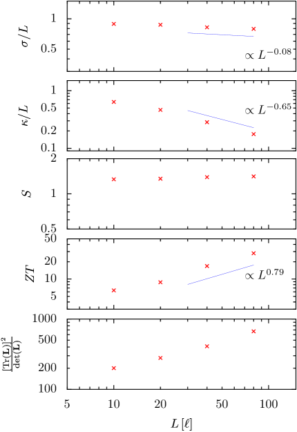
Figure 2: Thermoelectric transport properties. The quantities $\sigma/L,\kappa/L$, $ZT$, and $\frac{[{\rm Tr}({\bf L})]^{2}}{\det({\bf L})}$ show a power law dependence on the system size $L$.

In Fig. 2, we present our numerical results for the transport coefficients. A power law dependence for $\sigma/L$, $\kappa/L$, and $ZT$ is observed . In particular, the figure of merit $ZT$ increases with increasing the systems size, $ZT\propto L^{0.79}$. Correspondingly, the condition number ${[{\rm Tr}({\bf L})]^{2}}/{\det({\bf L})}$ (see Eq. (21)) diverges, as expected from the general theoretical considerations of Sec. 2.

These numerical results naturally raise a question: Is the mechanism leading to high $ZT$ quality factor for interacting gases related to the delta-like mechanism [5, 6] shortly discussed in Sec. 4 for the non-interacting ideal gas? To address this question, we measure the particle current at the position $x\in[0,L]$ as

$$J_{\rho}=\int_{0}^{\infty}dED(E),$$ (42)

$$D(E)\equiv D_{L}(E)-D_{R}(E),$$ (43)

where the “transmission function” $D_{L}(E)$ is the density of particles with energy $E$ crossing $x$ and coming from the left side, while $D_{R}(E)$ is the density of particles with energy $E$ from the right side. We inquire how $D(E)$ changes as a function of $L$, in particular if $D(E)$ becomes more and more delta-like (peaked in energy) when increasing $L$. The transmission function $D(E)$ is shown in Fig. 3, at $x=L/2$ and for different system sizes . There is no sign of narrowing of $D(E)$ when increasing the system size. We can therefore conclude that the mechanism leading to the large $ZT$ values observed in Fig. 2 must be different from the energy filtering discussed in Refs. [5, 6].

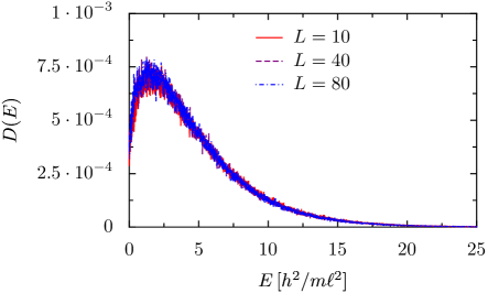
Figure 3: $D(E)$ calculated for $L=10,40$ and $80$.

To understand the mechanism, we first write the particle and energy currents as

$$J_{\rho}=\overline{v(x,t)\,\rho(x,t)},\quad J_{u}=\overline{\frac{1}{2}mv(x,t)^{3}\rho(x,t)},$$ (44)

where $x\in[0,L]$, the overbar denotes time-averaging, and $v(x,t)$, $\rho(x,t)$ are respectively the particles velocity and density at the position $x$ and time $t$. If the relaxation time scales for density and velocity are well separated, then expressions (44) can be approximated as:

$$J_{\rho}\sim\overline{v(x,t)}\times\overline{\rho(x,t)},~{}~{}~{}~{}~{}J_{u}\sim\overline{\frac{1}{2}mv(x,t)^{3}}\times\overline{\rho(x,t)}.$$ (45)

In our model, this is satisfied. For instance, in the case of $(\mu_{L},\mu_{R})=(0.24,0.16)\,[h^{2}/m\ell^{2}],T=3.0\,[h^{2}/m\ell^{2}k_{B}]$, and $L=40\,[\ell]$, we get at $x=L/2$ the time-averaged velocity $\overline{v(L/2,t)}\approx 0.010\,[h/m\ell]$, and the time-averaged density $\overline{\rho(L/2,t)}\approx 6.43\,[1/\ell]$, while $\overline{v(L/2,t)\,\rho(L/2,t)}\approx 0.0641\,[h/m\ell^{2}]$.

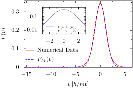
Figure 4: $F(v)$ calculated for the parameters $(\mu_{L},\mu_{R})=(0.24,0.16)\,[h^{2}/m\ell^{2}],T=3.0\,[h^{2}/m\ell^{2}k_{B}]$ with the system size $L=40$. The solid line corresponds to the the numerical data, at $x=L/2$. The mean velocity is $\overline{v(L/2,t)}\sim 0.010\,[h/m\ell]$. The dashed line is the modified Maxwell-Boltzmann distribution $F_{M}(v)$ which fits $F(v)$ with the parameters $\langle v\rangle=\overline{v(L/2,t)}=0.010[h/m\ell]$ and $\nu=1.15[h/m\ell]$. For these parameters, Eq.(47) yields $\langle v^{3}\rangle\sim 0.041$, which is comparable to the exact numerical data $\langle v^{3}\rangle\sim 0.047$. The inset shows the behavior of $F(v+\langle v\rangle)$ and $F(-v+\langle v\rangle)$ in the semi-log scale. These two curves completely overlap each other, as expected from Eq. (46). Note that the tails deviate from the Gaussian form.

From the discussion of Sec. 2, it is clear that $ZT$ diverges when $J_{u}\propto J_{\rho}$. According to Eq. (45), this is the case when $\overline{v^{3}}\propto\overline{v}$. Since we are interested in the steady-state transport properties and we are considering systems with the mixing property, it is natural to assume that the time-averages $\overline{v^{n}}$ equal the ensemble averages $\langle v^{n}\rangle\equiv\int_{-\infty}^{+\infty}dvv^{n}F(v)$, with $F(v)$ velocity distribution function for the steady state. At equilibrium ($T_{L}=T_{R}$, $\mu_{L}=\mu_{R}$), the system thermalizes and $F(v)$ is the Maxwell-Boltzmann distribution (22) at any $x$. In the linear response regime, we assume that $F(v)$ is given by a “modified Maxwell-Boltzmann distribution”,

$$F_{M}(v)=\sqrt{\frac{m^{\star}}{2\pi k_{B}T}}\exp\left(-\frac{m^{\star}(v-\langle v\rangle)^{2}}{2k_{B}T}\right),$$ (46)

where the mean velocity $\langle v\rangle$ and the effective mass $m^{\star}$ are fitting parameters, and $T\approx T_{L}\approx T_{R}$. That is to say, we assume that the out-of-equilibrium stationary distribution (46) differs from the equilibrium Maxwell-Boltzmann distribution only in the position $\langle v\rangle$ of the peak, while the Gaussian shape is unchanged. As shown in Fig. 4, such assumption is in good agreement with the numerically computed $F(v)$ close to the peak of the distribution, while the tails show deviations from (46). Nevertheless, such deviations do not affect too much the values of $\langle v\rangle$ and $\langle v^{3}\rangle$ and Eq. (46) is very convenient for analytical considerations and to unveil the mechanism at the origin of the large thermoelectric efficiencies observed in the hard-point gas model.

From Eq. (46) we obtain

$$\langle v^{3}\rangle=\langle v\rangle^{3}+3\nu^{2}\langle v\rangle,$$ (47)

where

$$\nu\equiv\sqrt{\frac{k_{B}T}{m^{\star}}}$$ (48)

is the width of distribution (46). We obtain $\langle v^{3}\rangle\propto\langle v\rangle$ when $\nu\gg\langle v\rangle$, that is, in the broad-distribution limit. It is clear from Fig. 4 that, for the one-dimensional interacting hard-point gas, indeed $\nu\gg\langle v\rangle$. 

6 Conclusions

We have studied numerically the coupled particle and energy transport in a prototype model of interacting one-dimensional gas: the disordered, hard-point gas. There is numerical evidence that the $ZT$ quality factor diverges with increasing the system size. We explain this result in terms of the emergence of a broad velocity distribution of the particles transmitted across the sample. This mechanism first of all requires local equilibrium, which is expected to take place in systems with the mixing property. We also make a couple of assumptions which are quite natural in many-body systems: the separation of the relaxation time scales of density and velocity in Eq. (45), and the modified Maxwell-Boltzmann form of the velocity distribution (46). On the other hand, since $ZT=(\sigma S^{2}/\kappa)T$ and Fig. 2 shows that the Seebeck coefficient is practically constant, the anomalous behavior of $\sigma$ and $\kappa$ [15] is crucial to obtain a diverging $ZT$. The relationship between the broad velocity-distribution mechanism and the anomalous behavior of the transport coefficients must be clarified. In particular, further investigations are required to understand whether this mechanism could be applied to systems with the mixing property but without anomalous transport. It might indeed be possible to find systems in which $\sigma$, $\kappa$ and $ZT$ eventually converge to finite but large values, when increasing the system size. Therefore, our mechanism could be also relevant in more realistic interacting systems with the mixing property.

References

- [1] G. Mahan, B. Sales, J. Sharp, Phys. Today 50 (March 1997), 42.
- [2] A. Majumdar, Science 303 (2004) 777.
- [3] M.S. Dresselhaus, G. Chen, M.Y. Tang, R.G. Yang, H. Lee, D.Z. Wang, Z.F. Ren, J.-P. Fleurial, P. Gogna, Adv. Mater. 19 (2007) 1043.
- [4] G.J. Snyder, E.R. Toberer, Nature Materials 7 (2008) 105.
- [5] G.D. Mahan, J.O. Sofo, Proc. Natl. Acad. Sci. USA 93 (1996) 7436.
- [6] T.E. Humphrey, R. Newbury, R.P. Taylor, H. Linke, Phys. Rev. Lett. 89 (2002) 116801; T.E. Humphrey, H. Linke, Phys. Rev. Lett. 94 (2005) 096601.
- [7] M. Terraneo, M. Peyrard, G. Casati, Phys. Rev. Lett. 88 (2002) 094302; B. Li, L. Wang, G. Casati, Phys. Rev. Lett. 93 (2004) 184301; D. Segal, A. Nitzan, Phys. Rev. Lett. 94 (2005) 034301; B. Hu, L. Yang, and Y. Zhang, Phys. Rev. Lett. 97 (2006) 124302; N. Yang, N. Li, L. Wang, B. Li, Phys. Rev. B 76, 020301(R) (2007); B. Li, L. Wang, G. Casati, Appl. Phys. Lett. 88 (2006) 143501; L. Wang and B. Li, Phys. World 21 (2008) 27; N. Li, F. Zhan, P. Hänggi, B. Li, Phys. Rev. E 80 (2009) 011125, and references therein.
- [8] G. Casati, C. Mejía-Monasterio, T. Prosen, Phys. Rev. Lett. 101 (2008) 016601.
- [9] G. Casati, L. Wang, T. Prosen, J. Stat. Mech. (2009) L03004.
- [10] H.B. Callen, Thermodynamics and an Introduction to Thermostatics (second edition), John Wiley & Sons, New York, 1985.
- [11] S.R. de Groot, P. Mazur, Non-Equilibrium Thermodynamics, Dover, New York, 1984.
- [12] P.L. Walstrom, Am. J. Phys. 56 (1988) 890.
- [13] C. Mejía-Monasterio, H. Larralde, F. Leyvraz, Phys. Rev. Lett. 86 (2001) 5417; H. Larralde, F. Leyvraz, C. Mejía-Monasterio, J. Stat. Phys. 113 (2003) 197.
- [14] K. Huang, Statistical Mechanics (second edition), John Wiley & Sons, New York, 1987, Sec. 6.6.
- [15] S. Lepri, R. Livi, A. Politi, Phys. Rep. 377 (2003) 1.