Master equation approach for interacting slow- and stationary-light polaritons

Abstract

A master equation approach for the description of dark-state polaritons in coherently driven atomic media is presented. This technique provides a description of light-matter interactions under conditions of electromagnetically induced transparency (EIT) that is well suited for the treatment of polariton losses. The master equation approach allows us to describe general polariton-polariton interactions that may be conservative, dissipative or a mixture of both. In particular, it enables us to study dissipation-induced correlations as a means for the creation of strongly correlated polariton systems. Our technique reveals a loss mechanism for stationary-light polaritons that has not been discussed so far. We find that polariton losses in level configurations with non-degenerate ground states can be a multiple of those in level schemes with degenerate ground states.

I INTRODUCTION

Photons are ideal carriers for quantum information over long distances. This is due to the large propagation speed of light and the fact that photons in free space do not interact with each other. On the other hand, the generation of highly entangled light fields and the realization of photon gates requires strong photon-photon interactions Nielsen and Chuang (2000). Nonlinear media can mediate an effective interaction between photons, but the strength of this induced coupling is usually weak. Thus the realization of strong photon-photon interactions is a major challenge in quantum information science. Similarly, strong photon-photon interactions are a key requirement for quantum optical implementations of highly correlated many-body systems Bloch et al. (2008). A substantial research effort  Hartmann et al. (2006); Hartmann et al. (2008a, b); Rossini and Fazio (2007); Angelakis et al. (2007); D.Gerace et al. (2006); haf (a, b); Carusotto et al. (2009); Fleischhauer et al. (2008); Chang et al. (2008); Kiffner and Hartmann (2010) is currently devoted to these systems where combined excitations of light and matter, i.e. polaritons, reproduce the dynamics of bosons with tunable mass and different interaction types. Several effects in correlated many-body systems were considered, including the realization of Bose-Hubbard models Hartmann et al. (2006); Hartmann et al. (2008b, a); Rossini and Fazio (2007); Angelakis et al. (2007), quantum transport haf (a, b), nonlinear effects in driven dissipative systems D.Gerace et al. (2006); Hartmann (2010), Bose-Einstein condensation Fleischhauer et al. (2008), and the realization of a Tonks-Girardeau gas Chang et al. (2008); Carusotto et al. (2009); Kiffner and Hartmann (2010) of polaritons.

Dark-state polaritons Fleischhauer and Lukin (2000, 2002); Lukin (2003) represent bosonic quasi-particles that arise in light-matter interactions under conditions of electromagnetically induced transparency (EIT) Fleischhauer et al. (2005). The generic EIT scheme consists of a gas comprised of three-level atoms in $\Lambda$ configuration that are driven by a strong control field and a weak probe field on separate transitions. EIT gives rise to a multitude of intriguing effects like the slowing and stopping of light Hau et al. (1999); Kash et al. (1999); Budker et al. (1999), the coherent storage and retrieval of light Liu et al. (2001a); Phillips et al. (2001); Fleischhauer and Lukin (2000, 2002); Dey and Agarwal (2003) and stationary light  André and Lukin (2002); Bajcsy et al. (2003); Zimmer et al. (2006, 2008); Moiseev and Ham (2005, 2006); Fleischhauer et al. (2008); Lin et al. (2009); Nikoghosyan and Fleischhauer (2009). Of particular relevance for quantum optical realizations of strongly correlated many-body systems is stationary light where the polaritons experience a quadratic dispersion relation like bosons in free space. Moreover, EIT in atomic four-level systems gives rise to a strongly enhanced Kerr nonlinearity for the probe fields Schmidt and Imamoǧlu (1996); Imamoǧlu et al. (1997); Harris and Yamamoto (1998); Harris and Hau (1998); Kang and Zhu (2003); Braje et al. (2004); Hartmann and Plenio (2007). This effect results in a two-particle contact interaction between the polaritons that can be conservative André et al. (2005); Chang et al. (2008) or dissipative Kiffner and Hartmann (2010).

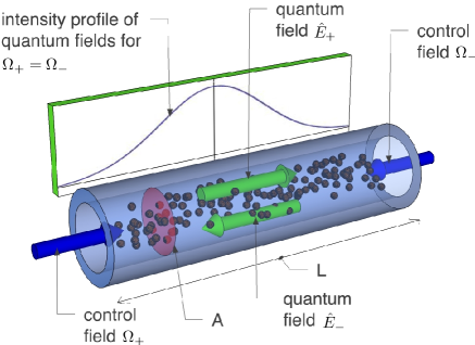
Figure 1: (Color online) Considered setup of $N$ atoms confined to an interaction volume of length $L$ and transverse area $A$. $\Omega_{\pm}$ are the Rabi frequencies of the classical control fields, and $\hat{E}_{\pm}$ are the quantum probe fields. A typical intensity profile of the quantum fields is shown for the case of stationary light where the control fields have the same intensity ($\Omega_{+}=\Omega_{-}$).

Experimental setups that show great promise for the realization of strongly correlated polariton systems are arrays of coupled microcavities doped with emitters Aoki et al. (2006); Wallraff et al. (2004); leib:10 ; Hennessy et al. (2007); Trupke et al. (2007) or optical fibers that couple to atoms Bajcsy et al. (2009); vet . In general, strong light-matter interactions require the confinement of light to small interaction volumes. Here we consider the experimental setup Bajcsy et al. (2009) shown in Fig. 1, where photons and atoms are simultaneously confined to the hollow core of a photonic-crystal fiber, and the level scheme of each atom is shown in Fig. 2. Since the light-guiding core of the optical fiber is of the same order of magnitude as the optical wavelength, the fiber represents a one-dimensional waveguide for the optical fields. Note that a second potential realization is comprised of the experimental setup in vet , where multi-color evanescent light fields surrounding an optical nanofiber couple to atoms trapped in an optical lattice.

Existing descriptions Fleischhauer and Lukin (2000, 2002) of dark-state polaritons in EIT systems are based on a Heisenberg-Langevin approach for the polariton field operator. Here we present a different approach and derive a master equation for the reduced density operator of dark-state polaritons. The master equation technique facilitates the treatment of polariton losses and allows one to account for general polariton-polariton interactions that may be conservative, dissipative or a mixture of both. This is an important achievement since it opens up the possibility to study dissipation-induced correlations Syassen et al. (2008); Dürr et al. (2009) in polariton systems. Dissipative polariton-polariton interactions are promising in the quest for highly correlated systems since they can be considerably stronger than their conservative counterparts Kiffner and Hartmann (2010). Second, our method reveals an additional loss term for stationary-light polaritons whose importance depends on the structure of the atomic level scheme and that was not discussed in the literature yet.

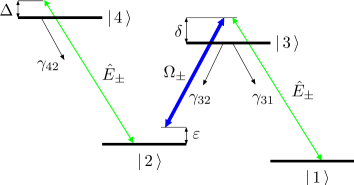
Figure 2: (Color online) Atomic level scheme. $\gamma_{ij}$ is the full decay rate on the $|i\rangle\leftrightarrow|j\rangle$ transition, $\delta$ and $\Delta$ label the detuning of the probe fields with states $|3\rangle$ and $|4\rangle$, respectively, and $\varepsilon$ is the two-photon detuning.

This paper is organized as follows. In Sec. II we set up a master equation for the atoms interacting with the quantized probe and classical control fields inside the 1D waveguide, see Figs. 1 and 2. We then transfer the original master equation into a master equation solely for dark-state polaritons. This process is detailed in Sec. III and consists of four steps. First, we show that the entire problem can be described in terms of bosonic quasi-particles if the number of atoms is much larger than the number of probe field photons, see Sec. III.1. The concept of dark-state polaritons is introduced in Sec. III.2, and the formulation of the original master equation of Sec. II in terms of dark-state polaritons and all other excitations is presented in Sec. III.3. In the final step of the derivation we trace out all excitations except for the dark-state polaritons, see Sec. III.4. The master equation for dark-state polaritons under conditions of stationary light and for arbitrary (conservative or dissipative) polariton-polariton interactions is presented in Sec. IV. Here we summarize all conditions that grant the validity of our approach. The special case where the level scheme in Fig. 2 is reduced to the $\Lambda$ subsystem is discussed in Sec. IV.1. We compare the predictions of our master equation to the results of a numerical integration of Maxwell-Bloch equations and find excellent agreement. The full master equation including the most general form of polariton-polariton interactions is covered in Sec. IV.2, and the mapping to the dissipative Lieb-Liniger model is outlined in Sec. IV.3. Finally, in Sec. IV.4 we compare the advantages and disadvantages between the atomic level schemes in Figs. 2 and 5 that both give rise to the same master equation for dark-state polaritons.

II DESCRIPTION OF THE SYSTEM

We start with a more detailed description of our one-dimensional model shown in Figs. 1 and 2. Each of the $N$ atoms interacts with control and probe fields denoted by $\Omega_{\pm}$ and $\hat{E}_{\pm}$, respectively. The control fields of frequency $\omega_{c}$ are treated classically and $\Omega_{+}$ ($\Omega_{-}$) labels the Rabi frequency of the control field propagating in the positive (negative) $z$ direction. In addition, we assume that the control fields are spatially homogeneous and that the Rabi frequencies $\Omega_{\pm}$ are real. The probe fields $\hat{E}_{+}$ and $\hat{E}_{-}$ are quantum fields that propagate in the positive and negative $z$ direction, respectively. They are defined as

$$\hat{E}_{\pm}(z)=\sum_{k}a_{\pm k_{c}+k}e^{i(\pm k_{c}+k)z},$$ (1)

where $a_{\pm k_{c}+k}$ are photon annihilation operators of a mode with frequency $\omega_{\pm k_{c}+k}$ and $k_{c}$ ($-k_{c}$) is the wave number of the control field $\Omega_{+}$ ($\Omega_{-}$). We assume that the wave numbers $k$ satisfy $|k|\ll k_{c}$ which implies that the envelope of the quantum fields varies slowly on a lengthscale defined by the wavelength of the optical fields.

We model the time evolution of the atoms and the quantized probe fields by a master equation Breuer and Petruccione (2006) for their density operator $\varrho$,

$$\dot{\varrho}=-\frac{i}{\hbar}[H,\varrho]+\mathcal{L}_{\gamma}\varrho,$$ (2)

where the system Hamiltonian $H=H_{0}+H_{\Lambda}+H_{\text{NL}}$ is comprised of three parts. $H_{0}$ describes the free time evolution of the atoms and the probe fields, and $H_{\Lambda}$ accounts for the interaction of the probe and control fields with the $\Lambda$-subsystem formed by states $|1\rangle$, $|2\rangle$ and $|3\rangle$. On the other hand, $H_{\text{NL}}$ accounts for the coupling of the probe fields to the $|2\rangle\leftrightarrow|4\rangle$ transition and results in a nonlinear coupling between probe field photons Schmidt and Imamoǧlu (1996); Imamoǧlu et al. (1997); Harris and Yamamoto (1998); Harris and Hau (1998); Kang and Zhu (2003); Braje et al. (2004); Hartmann and Plenio (2007). In a rotating frame that removes the time-dependence of the classical laser fields, $H_{0}$, $H_{\Lambda}$ and $H_{\text{NL}}$ are given by

$$H_{0}= -\hbar\sum_{k}(\omega_{p}-\omega_{k_{c}+k})a^{\dagger}_{k_{c}+k}a_{k_{c}+k}$$ (3)

$$-\hbar\sum_{k}(\omega_{p}-\omega_{-k_{c}+k})a^{\dagger}_{-k_{c}+k}a_{-k_{c}+k}$$

$$-\hbar\sum_{\mu=1}^{N}\left[\varepsilon A_{22}^{(\mu)}+\delta A_{33}^{(\mu)}+(\Delta+\varepsilon)A_{44}^{(\mu)}\right],$$

$$H_{\Lambda}= -\hbar\sum_{\mu=1}^{N}\Big{\{}S_{32}^{(\mu)}\left[\Omega_{+}e^{ik_{c}z_{\mu}}+\Omega_{-}e^{-ik_{c}z_{\mu}}\right]$$ (4)

$$\hskip 14.22636pt+g_{1}S_{31}^{(\mu)}\left[\hat{E}_{+}(z_{\mu})+\hat{E}_{-}(z_{\mu})\right]\Big{\}}+\text{h.c.},$$

$$H_{\text{NL}}= -\hbar g_{2}\sum_{\mu=1}^{N}S_{42}^{(\mu)}\left[\hat{E}_{+}(z_{\mu})+\hat{E}_{-}(z_{\mu})\right]+\text{h.c.}\,.$$ (5)

Here $A_{ii}^{\mu}$ and $S_{ij}^{(\mu)}$ are projection and transition operators of atom $\mu$ at position $z_{\mu}$, respectively,

$$A_{ii}^{\mu}=|i_{\mu}\rangle\langle i_{\mu}|, S_{ij}^{(\mu)}=|i_{\mu}\rangle\langle j_{\mu}|\quad(i\not=j),$$ (6)

$\omega_{p}$ is the central frequency of the probe pulse, and $g_{1}$ ($g_{2}$) is the single-photon Rabi frequency on the $|3\rangle\leftrightarrow|1\rangle$ ($|4\rangle\leftrightarrow|2\rangle$) transition. The detuning of the probe field with respect to the transition $|3\rangle\leftrightarrow|1\rangle$ ($|4\rangle\leftrightarrow|2\rangle$) is labeled by $\delta$ ($\Delta$), and $\varepsilon$ is the two-photon detuning,

$$\delta=\omega_{p}-\omega_{31},\quad\Delta=\omega_{p}-\omega_{42},\quad\varepsilon=\omega_{p}-\omega_{c}-\omega_{2}.$$ (7)

Here the energy of level $|i\rangle$ is $\hbar\omega_{i}$ (we set $\omega_{1}=0$) and transition frequencies are denoted by $\omega_{ij}=\omega_{i}-\omega_{j}$. The term $\mathcal{L}_{\gamma}\varrho$ in Eq. (2) accounts for spontaneous emission from states $|3\rangle$ and $|4\rangle$,

$$\mathcal{L}_{\gamma}\varrho= -\frac{\gamma_{31}}{2}\sum\limits_{\mu=1}^{N}\left(A_{33}^{(\mu)}\varrho+\varrho A_{33}^{(\mu)}-2S_{13}^{(\mu)}\varrho S_{31}^{(\mu)}\right)$$ (8)

$$-\frac{\gamma_{32}}{2}\sum\limits_{\mu=1}^{N}\left(A_{33}^{(\mu)}\varrho+\varrho A_{33}^{(\mu)}-2S_{23}^{(\mu)}\varrho S_{32}^{(\mu)}\right)$$

$$-\frac{\gamma_{42}}{2}\sum\limits_{\mu=1}^{N}\left(A_{44}^{(\mu)}\varrho+\varrho A_{44}^{(\mu)}-2S_{24}^{(\mu)}\varrho S_{42}^{(\mu)}\right),$$

where $\gamma_{ij}$ is the full decay rate on the transition $|i\rangle\leftrightarrow|j\rangle$ (see Fig. 1). Finally, we introduce the parameter

$$\Delta\omega=\omega_{p}-\omega_{c}=\omega_{2}+\varepsilon$$ (9)

which describes the frequency difference between the probe and control fields. Note that $\Delta\omega$ is practically equal to the frequency splitting $\omega_{2}$ between the ground states $|1\rangle$ and $|2\rangle$ if the two-photon detuning $\varepsilon$ is small. Next we outline the approach we developed to reduce the master equation (2) for the atoms and quantized probe fields into a master equation solely for dark-state polaritons Fleischhauer and Lukin (2000), formed by collective excitations of photons and atoms.

III MASTER EQUATION FOR DARK-STATE POLARITONS: DERIVATION

Here we show that the master equation (2) can be simplified considerably if we assume that almost all atoms are in state $|1\rangle$ and that the total number of photons is much smaller than the number of atoms $N$. This assumption allows us to study the system dynamics entirely in terms of independent bosonic quasi-particle excitations, see Sec. III.1. A second simplification is made possible by the concept of dark-state polaritons Fleischhauer and Lukin (2000, 2002) introduced in Sec. III.2. Dark-state polaritons are bosonic quasi-particles that decay only indirectly via the coupling to other bosonic modes that are termed bath excitations. In the so-called slow-light regime, this coupling is much slower than the decay of the bath excitations which is of the order of the decay rates of the excited states $|3\rangle$ and $|4\rangle$. The existence of these two different time scales enables us to derive a Markovian master equation for the reduced density operator of the dark-state polaritons as outlined in Sec. III.4. Throughout this Section, all technical details and lengthy definitions are moved to the Appendix.

III.1 BOSONIZATION

Here we show that the system described in Sec. II can be mapped to a much simpler system if almost all atoms are in state $|1\rangle$ and if the total number of photons is much smaller than the number of atoms $N$. We begin with the description of a simple system that consists of $M$ bosonic modes. The annihilation operator of mode $i$ is given by $O_{i}$ ($i\in\{1,\ldots,M\}$) and $\mathcal{O}=\{O_{1},\ldots,O_{M}\}$ denotes the set of all operators that obey the commutation relations

$$\left[\hat{O}_{i},\hat{O}_{j}^{\dagger}\right]=\delta(i,j),\quad\left[\hat{O}_{i},\hat{O}_{j}\right]=0.$$ (10)

If $|0\rangle$ is the vacuum state of the system, it follows that

$$|\{n_{1},\ldots,n_{M}\}\rangle=\prod_{i=1}^{M}\frac{1}{\sqrt{n_{i}!}}\big{(}\hat{O}_{i}^{\dagger}\big{)}^{n_{i}}|0\rangle$$ (11)

is a normalized state with $n_{i}$ excitations in mode $i$ and a total number of $\sum_{i=1}^{M}n_{i}$ excitations. Furthermore, we note that the total state space of $M$ bosonic modes is the tensor product of the state spaces $\mathcal{H}_{i}$ associated with the individual modes,

$$\mathcal{H}_{\text{osc}}=\mathcal{H}_{1}\otimes\mathcal{H}_{2}\otimes\ldots\otimes\mathcal{H}_{M}.$$ (12)

Next we show how the system of Sec. II can be mapped to this simple model outlined in Eqs. (10)-(12). First we define a vacuum state where all probe field modes are empty and all atoms are in state $|1\rangle$,

$$|0\rangle=|\{0\}_{\text{phot}};1_{1},\ldots,1_{N}\rangle.$$ (13)

Second, we define the following operators ($m\in\mathds{Z}$)

$$A_{k}=a_{k_{c}+k}\sin\varphi+a_{-k_{c}+k}\cos\varphi,$$ (14)

$$D_{k}=a_{k_{c}+k}\cos\varphi-a_{-k_{c}+k}\sin\varphi,$$ (15)

$$X_{k}(m)=\frac{1}{\sqrt{N}}\sum_{\mu=1}^{N}S_{12}^{(\mu)}e^{-i(mk_{c}+k)z_{\mu}},$$ (16)

$$H_{k}(m)=\frac{1}{\sqrt{N}}\sum_{\mu=1}^{N}S_{13}^{(\mu)}e^{-i(mk_{c}+k)z_{\mu}},$$ (17)

$$I_{k}(m)=\frac{1}{\sqrt{N}}\sum_{\mu=1}^{N}S_{14}^{(\mu)}e^{-i(mk_{c}+k)z_{\mu}},$$ (18)

where $k=n2\pi/L$ ($n\in\mathds{Z}$) and $A_{k}$ ($D_{k}$) is a sum (difference) of two counter-propagating probe field modes. Since $a_{\pm k_{c}+k}$ are photon annihilation operators, it follows that $A_{k}$ and $D_{k}$ obey bosonic commutation relations. The angle $\varphi$ depends on the relative strength of the Rabi frequencies $\Omega_{+}$ and $\Omega_{-}$ and is defined by Zimmer et al. (2006, 2008)

$$\sin\varphi=\frac{\Omega_{+}}{\sqrt{\Omega_{+}^{2}+\Omega_{-}^{2}}},\quad\cos\varphi=\frac{\Omega_{-}}{\sqrt{\Omega_{+}^{2}+\Omega_{-}^{2}}}.$$ (19)

The operator $X_{k}(m)$ describes a collective spin coherence that is slowly oscillating for $m=0$ and fast oscillating for $m\not=0$. The operators $H_{k}^{\dagger}(m)$ and $I_{k}^{\dagger}(m)$ create an excitation in the excited states $|3\rangle$ and $|4\rangle$, respectively. Next we show that the operators defined in Eqs. (16)-(18) obey bosonic commutation relations for all wave numbers $k$ and all $m\in\mathds{Z}$ if almost all atoms are in state $|1\rangle$. As an example, we discuss the commutation relations for $X_{k}(m)$. Within a manifold with fixed $m$, we find

$$\left[X_{k}(m),X_{p}^{\dagger}(m)\right] =\frac{1}{N}\sum\limits_{\mu=1}^{N}\left(A_{11}^{(\mu)}-A_{22}^{(\mu)}\right)e^{i(p-k)z_{\mu}}$$ (20)

$$\approx\frac{1}{N}\sum\limits_{\mu=1}^{N}e^{i(p-k)z_{\mu}}$$ (21)

$$\approx\frac{1}{L}\int\limits_{0}^{L}dze^{i(p-k)z}=\delta(k,p)\,,$$

where we set $A_{11}^{(\mu)}\approx\mathds{1}$ and $A_{22}^{(\mu)}\approx 0$ since almost all atoms are in state $|1\rangle$. Furthermore, we employed that the mean distance between atoms is much smaller than $1/|k|$ for all relevant wavenumbers $k$ contributing to the slowly varying envelopes of the control fields. In the case $m\not=n$, we find

$$\left[X_{k}(m),X_{p}^{\dagger}(n)\right] \approx\frac{1}{N}\sum\limits_{\mu=1}^{N}e^{i[(p-k)+(n-m)k_{c}]z_{\mu}}.$$ (22)

In contrast to Eq. (20), the sum cannot be converted into an integral since the mean spacing between the atoms is much larger than $1/k_{c}$ for realistic densities, where $k_{c}$ is the wavenumber of an optical transition. However, the sum in Eq. (22) represents the average of random numbers on the unit circle in the complex plain, which is zero in the limit $N\rightarrow\infty$. We can thus set $[X_{k}(m),X_{p}^{\dagger}(n)]\approx 0$ for $m\not=n$. Since $[X_{k}(m),X_{p}(n)]=0$, it follows that the operators $X_{k}(m)$ obey bosonic commutation relations if almost all atoms are in state $|1\rangle$, and corrections scale with $1/N$. The same result is found for $H_{k}(m)$ and $I_{k}(m)$. Furthermore, we point out that $X_{k}(m)$, $H_{k}(m)$ and $I_{k}(m)$ describe independent excitations up to corrections that scale with $1/N$, i.e., $[X_{k}(m),H_{p}^{\dagger}(n)]\approx 0$, $[X_{k}(m),I_{p}^{\dagger}(n)]\approx 0$ and $[I_{k}(m),H_{p}^{\dagger}(n)]\approx 0$.

In summary, we can introduce the set of bosonic operators

$$\mathcal{O}=\{A_{k},D_{k},X_{k}(m),H_{k}(m),I_{k}(m)\}_{\genfrac{}{}{0.0pt}{2}{k\hskip 11.38092pt}{m\in\mathds{Z}}}$$ (23)

if almost all atoms are in state $|1\rangle$. This condition can be met if the total state space $\mathcal{H}_{\text{tot}}$ of the system is restricted to the subspace

$$\mathcal{H}_{\text{FE}}=\text{Span}\left\{|\{n_{1},\ldots,n_{M}\}\rangle\;\big{|}\;\sum\limits_{i=1}^{M}n_{i}\ll N\right\}$$ (24)

that is spanned by states with much less excitations than number of atoms $N$. From a physical point of view, the system dynamics will be restricted to this subspace if the number of photons is much smaller than the number of atoms, and if initially almost all atoms are in state $|1\rangle$. In Appendix A, we show that the Hamiltonian $H$ and the decay term $\mathcal{L}_{\gamma}\varrho$ can be expressed entirely in terms of the bosonic operators in Eq. (23) if the state space is restricted to $\mathcal{H}_{\text{FE}}$. We denote the density operator in $\mathcal{H}_{\text{FE}}$ by $\tilde{\varrho}$, and the master equation (2) in $\mathcal{H}_{\text{FE}}$ can be written as

$$\dot{\tilde{\varrho}}=-\frac{i}{\hbar}[\tilde{H},\tilde{\varrho}]+\tilde{\mathcal{L}}_{\gamma}\tilde{\varrho},$$ (25)

where $\tilde{H}=\tilde{H}_{0}+\tilde{H}_{\Lambda}+\tilde{H}_{\text{NL}}$. The operators $\tilde{H}_{0}$, $\tilde{H}_{\Lambda}$, $\tilde{H}_{\text{NL}}$ and $\tilde{\mathcal{L}}_{\gamma}\tilde{\varrho}$ are defined in Eqs. (84), (86), (87) and (88), respectively. These operators approximate their counterparts without tilde in the subspace $\mathcal{H}_{\text{FE}}$ and are comprised of the bosonic operators in Eq. (23).

III.2 DARK-STATE POLARITONS

The interaction Hamiltonian $H_{\Lambda}$ of the $\Lambda$-subsystem has the important property that a certain class of its eigenstates are so-called dark states $|D\rangle$. These states are called dark since they do not contain a contribution of the excited state $|3\rangle$ and are thus immune against spontaneous emission. A simple example for a dark state is given by

$$|D\rangle=\psi_{k}^{\dagger}|0\rangle,$$ (26)

where the unique definition of the operator $\psi_{k}$ is Zimmer et al. (2008)

$$\psi_{k}=A_{k}\cos\theta-X_{k}\sin\theta.$$ (27)

In this equation, $A_{k}$ is a superposition of two counter-propagating probe field modes, and $X_{k}=X_{k}(0)$ describes a slowly varying collective spin coherence. The mixing angle $\theta$ determines the weight of the photonic ($A_{k}$) and atomic ($X_{k}$) components contributing to $\psi_{k}$ and is defined as Fleischhauer and Lukin (2000, 2002); André and Lukin (2002); Zimmer et al. (2006, 2008)

$$\sin\theta=\frac{\sqrt{N}g_{1}}{\Omega_{0}},\;\cos\theta=\frac{\sqrt{\Omega_{+}^{2}+\Omega_{-}^{2}}}{\Omega_{0}},\;$$ (28)

$$\Omega_{0}=\sqrt{Ng_{1}^{2}+\Omega_{+}^{2}+\Omega_{-}^{2}}.$$ (29)

A short calculation shows that $|D\rangle$ in Eq. (26) is an eigenstate of $H_{\Lambda}$ in Eq. (4) with eigenvalue zero, i.e., $H_{\Lambda}|D\rangle=0$. Furthermore, Eq. (27) implies that $|D\rangle$ does not contain a contribution of the excited state $|3\rangle$. It follows that state $|D\rangle$ is indeed a dark state of the interaction Hamiltonian $H_{\Lambda}$. Note, however, that $|D\rangle$ is not an eigenstate of the remaining parts $H_{0}$ and $H_{\text{NL}}$ of the full Hamiltonian, and these terms give rise to a non-trivial time evolution of the dark-state polaritons.

The results of Sec. III.1 and Eq. (27) imply that the operators $\psi_{k}$ obey bosonic commutation relations in $\mathcal{H}_{\text{FE}}$,

$$\left[\psi_{k},\psi_{p}^{\dagger}\right]\approx\delta(k,p),$$ (30)

and the quasi-particles associated with these excitations are termed dark-state polaritons. It follows from Eq. (30) that

$$|D\rangle=\prod_{k}\frac{1}{\sqrt{n_{k}!}}\big{(}\psi_{k}^{\dagger}\big{)}^{n_{k}}|0\rangle$$ (31)

represents a normalized dark state with $\sum_{k}n_{k}$ excitations. We emphasize that the photonic part $A_{k}$ of $\psi_{k}$ contains a pair of counter-propagating probe field modes that are grouped around the wavenumbers of the control fields $\pm k_{c}$ rather than the mean wavenumbers $\pm k_{p}$ of the probe fields, see Eq. (14). Note that the states in Eq. (31) would not be true dark states if the probe field modes in $A_{k}$ were grouped around $\pm k_{p}$ and if both $\Omega_{+}$ and $\Omega_{-}$ were different from zero.

III.3 BOSONIZATION WITH DARK-STATE POLARITONS

We have shown in Sec. III.1 that the master equation (2) can be formulated in terms of bosonic modes if the system dynamics is restricted to the subspace $\mathcal{H}_{\text{FE}}$. Here we restate this model in terms of long-lived dark-state polaritons introduced in Sec. III.2. With the definition of the bright-state polariton Fleischhauer et al. (2008)

$$\phi_{k}=A_{k}\sin\theta+X_{k}\cos\theta$$ (32)

and the inverse relations of Eqs. (27) and (32), we replace the operators $A_{k}$ and $X_{k}(0)$ in $\mathcal{O}$ [see Eq. (23)] by $\psi_{k}$ and $\phi_{k}$. This allows us to write the subspace $\mathcal{H}_{\text{FE}}$ in Eq. (24) as the tensor product of the state space $\mathcal{H}_{\text{S}}$ of dark-state polaritons and the state space $\mathcal{H}_{\text{B}}$ of all other modes termed bath excitations,

$$\mathcal{H}_{\text{FE}}=\mathcal{H}_{\text{S}}\otimes\mathcal{H}_{\text{B}}\,.$$ (33)

The partition of all bosonic modes into dark-state polaritons and bath excitations is motivated by our aim to derive a master equation for the long-lived dark-state polaritons only, see Sec. III.4.

In the following, we assume that the Rabi frequencies of the control fields are identical and set

$$\Omega_{c}=\Omega_{+}=\Omega_{-}.$$ (34)

With this choice, $H_{\Lambda}$ gives rise to the stationary light phenomenon André and Lukin (2002); Bajcsy et al. (2003) that allows us to trap the probe field inside the medium. Note that any other choice of the Rabi frequencies $\Omega_{\pm}$ can be treated within the formalism introduced here, and in these cases the calculation follows exactly the same route as detailed below. If the operators $A_{k}$ and $X_{k}(0)$ in the master equation (25) are replaced by $\psi_{k}$ and $\phi_{k}$, we obtain (see Appendix B)

$$\dot{\tilde{\varrho}}=-\frac{i}{\hbar}[H_{\text{S}},\tilde{\varrho}]-\frac{i}{\hbar}[V,\tilde{\varrho}]+\mathcal{L}_{\text{B}}\varrho,$$ (35)

where

$$H_{\text{S}}=-\hbar(\sin\theta\varepsilon+\cos^{2}\theta)\sum\limits_{k}\psi_{k}^{\dagger}\psi_{k}$$ (36)

describes the free time evolution of the dark-state polaritons. Here we choose a small two-photon detuning

$$\varepsilon=-\cot^{2}\theta\Delta\omega$$ (37)

such that $H_{\text{S}}=0$. The dynamics of the bath excitations is governed by the Liouvillian

$$\mathcal{L}_{\text{B}}\tilde{\varrho}=-\frac{i}{\hbar}[H_{\text{B}},\tilde{\varrho}]+\mathcal{L}_{\gamma}^{(\text{B})}\tilde{\varrho},$$ (38)

where $H_{\text{B}}$ accounts for the unitary time evolution of the bath modes and the decay of bath excitations is determined by $\mathcal{L}_{\gamma}^{(\text{B})}\tilde{\varrho}$. The interaction between dark-state polaritons and other excitations in $\mathcal{H}_{\text{B}}$ is described by the interaction Hamiltonian $V$. The definitions of $H_{\text{B}}$, $\mathcal{L}_{\gamma}^{(\text{B})}\tilde{\varrho}$ and $V$ are provided in Appendix B.

The decay term $\mathcal{L}_{\gamma}^{(\text{B})}\tilde{\varrho}$ results in a finite lifetime of the bath excitations that is of the order of the lifetimes of the excited states $|3\rangle$ and $|4\rangle$. On the other hand, the dark-state polaritons decay only indirectly via the coupling to bath excitations mediated by $V$. In the slow light limit, this coupling is much slower than the decay of the bath excitations. This existence of two different time scales opens up the possibility to derive a Markovian master equation for the dark-state polaritons alone, and this procedure is outlined in the next Section III.4.

III.4 ELIMINATION OF THE BATH

In the previous Sections III.1-III.3 we achieved to transform the initial master equation (2) within the subspace $\mathcal{H}_{\text{FE}}$ into a master equation for long-lived dark-state polaritons and fast-decaying bath excitations. Here we are especially interested in the quantum state $\varrho_{\text{D}}$ of the dark-state polaritons that is obtained from $\tilde{\varrho}$ by a partial trace over all excitations except for the dark state polaritons. We derive the corresponding master equation for $\varrho_{\text{D}}$ from Eq. (35) via projection operator techniques Breuer and Petruccione (2006) and assume that the initial state of the system factorizes into a product of the initial polariton state $\varrho_{\text{D}}$ and the vacuum state $\varrho_{\text{B}}$ of the bath modes,

$$\tilde{\varrho}(t=0)=\varrho_{\text{D}}\otimes\varrho_{\text{B}}.$$ (39)

Furthermore, we employ the Born-Markov approximation Breuer and Petruccione (2006) and obtain

$$\dot{\varrho_{\text{D}}} =-\mathcal{S}(\varrho_{\text{D}})+\text{h.c.},$$ (40)

where

$$\mathcal{S}(\varrho_{\text{D}}) =\frac{1}{\hbar^{2}}\int\limits_{0}^{\infty}d\tau\text{Tr}_{\text{B}}\left\{\left[V,e^{\mathcal{L}_{\text{B}}\tau}V\varrho_{\text{D}}\otimes\varrho_{\text{B}}\right]\right\}.$$ (41)

The application of the Born-Markov approximation requires that the coupling of the dark-state polaritons to bath excitations is sufficiently weak and in particular small as compared to the decay rate of bath excitations. Conditions for the validity of the Born-Markov approximation as well as the assumption in Eq. (39) are discussed in Sec. IV and Appendix C. In order to outline the evaluation of Eq. (41), we write $V$ as

$$V=V^{(+)}+V^{(-)},$$ (42)

where the rising and lowering parts of $V$ are defined as

$$V^{(+)}=\sum\limits_{i}B_{i}^{\dagger}S_{i}\,,\qquad V^{(-)}=\sum\limits_{i}B_{i}S_{i}^{\dagger},$$ (43)

respectively. In this equation, $S_{i}$ represents a system operator comprised of dark-state polaritons, and $B_{i}$ is a bath operator. Since we assume that the bath is initially in its vacuum state, we have $V^{(-)}\varrho_{\text{B}}=0$ which allows us to replace $V\varrho_{\text{B}}$ by $V^{(+)}\varrho_{\text{B}}$ in Eq. (41). In addition, the second interaction Hamiltonian $V$ in Eq. (41) can be replaced by $V^{(-)}$ since the contribution of $V^{(+)}$ is negligible, see Appendix C. We thus arrive at

$$\mathcal{S}(\varrho_{\text{D}}) =\frac{1}{\hbar^{2}}\int\limits_{0}^{\infty}d\tau\text{Tr}_{\text{B}}\left\{\left[V^{(-)},e^{\mathcal{L}_{\text{B}}\tau}V^{(+)}\varrho_{\text{D}}\otimes\varrho_{\text{B}}\right]\right\}$$

$$=\frac{1}{\hbar^{2}}\sum\limits_{i,j}\int\limits_{0}^{\infty}d\tau\text{Tr}_{\text{B}}\left\{B_{i}e^{\mathcal{L}_{\text{B}}\tau}B_{j}^{\dagger}\varrho_{\text{B}}\right\}$$ (44)

$$\hskip 85.35826pt\times\left(S_{i}^{\dagger}S_{j}\varrho_{\text{D}}-S_{j}\varrho_{\text{D}}S_{i}^{\dagger}\right),$$

and the evaluation of the bath correlation functions $\text{Tr}_{\text{B}}\{B_{i}\exp[\mathcal{L}_{\text{B}}\tau]B_{j}^{\dagger}\varrho_{\text{B}}\}$ is presented in Appendix C. The final result for the master equation (40) is discussed in the next Section IV.

IV MASTER EQUATION FOR DARK-STATE POLARITONS: RESULTS

The master equation (2) in Sec. II describes the interaction of classical control and quantized probe fields with $N$ atoms. In Sec. III we demonstrated that this master equation can be converted into a master equation for the reduced density operator $\varrho_{\text{D}}$ of dark-state polaritons. For equally strong control fields [see Eq. (34)] and in the slow-light limit $\cos^{2}\theta\ll 1$ [see Eq. (29)], we obtain

$$\dot{\varrho}_{\text{D}}= -\frac{i}{\hbar}[H_{\text{nd}},\varrho_{\text{D}}]-\frac{i}{\hbar}[H_{3},\varrho_{\text{D}}]-\frac{i}{\hbar}[H_{4},\varrho_{\text{D}}]-\frac{\Gamma}{2\Omega_{0}^{2}}\cos^{2}\theta\sum\limits_{k}\omega_{k}^{2}\left(\psi_{k}^{\dagger}\psi_{k}\varrho_{\text{D}}+\varrho_{\text{D}}\psi_{k}^{\dagger}\psi_{k}-2\psi_{k}\varrho_{\text{D}}\psi_{k}^{\dagger}\right)$$ (45)

$$-\frac{\Gamma}{2\Omega_{0}^{2}}\Delta\omega^{2}\cos^{2}\theta\sum\limits_{k}\left(\psi_{k}^{\dagger}\psi_{k}\varrho_{\text{D}}+\varrho_{\text{D}}\psi_{k}^{\dagger}\psi_{k}-2\psi_{k}\varrho_{\text{D}}\psi_{k}^{\dagger}\right)$$

$$-\frac{g_{2}^{2}\gamma_{42}/2}{\Delta_{\theta}^{2}+\gamma_{42}^{2}/4}\cos^{2}\theta\,\sum\limits_{k,p,q}\left(\psi_{p}^{\dagger}\psi_{k-p}^{\dagger}\psi_{q}\psi_{k-q}\varrho_{\text{D}}+\varrho_{\text{D}}\psi_{p}^{\dagger}\psi_{k-p}^{\dagger}\psi_{q}\psi_{k-q}-2\psi_{q}\psi_{k-q}\varrho_{\text{D}}\psi_{p}^{\dagger}\psi_{k-p}^{\dagger}\right),$$

where

$$H_{\text{nd}}=-\hbar\frac{\delta}{\Omega_{0}^{2}}\Delta\omega^{2}\,\cos^{2}\theta\sum\limits_{k}\psi_{k}^{\dagger}\psi_{k},$$ (46)

$$H_{3}=-\hbar\frac{\delta}{\Omega_{0}^{2}}\cos^{2}\theta\sum\limits_{k}\omega_{k}^{2}\psi_{k}^{\dagger}\psi_{k},$$ (47)

$$H_{4}=\frac{\hbar\Delta_{\theta}g_{2}^{2}}{\Delta_{\theta}^{2}+\gamma_{42}^{2}/4}\cos^{2}\theta\sum\limits_{k,p,q}\psi_{p}^{\dagger}\psi_{k-p}^{\dagger}\psi_{q}\psi_{k-q}.$$ (48)

Here $\Delta\omega=\omega_{p}-\omega_{c}$ is the frequency difference between the probe and control fields,

$$\Delta_{\theta}=\Delta-\cot^{2}\theta\Delta\omega,$$ (49)

and $\Gamma=\gamma_{31}+\gamma_{32}$ is the full decay rate of state $|3\rangle$.

Next we summarize the conditions under which Eq. (45) holds. First of all, we note that the two-photon detuning $\varepsilon$ is constrained by Eq. (37), and it was assumed that $\Omega_{0}$ defined in Eq. (29) is large as compared to the decay rates of the excited states and the detuning with state $|3\rangle$,

$$\Omega_{0}\gg\Gamma,\gamma_{42},|\delta|.$$ (50)

A key assumption in the derivation of Eq. (45) is that the number of atoms is much larger than the number of photons, and that initially almost all atoms are in state $|1\rangle$. This condition is a prerequisite for the bosonization described in Sec. III.1. Furthermore, it was assumed in Sec. III.4 that initially all bath modes are in the vacuum state, and that the initial density operator of the total system factorizes, see Eq. (39). These conditions can be met if the initial dark-state polariton state is prepared via the slowing and stopping of a probe pulse Hau et al. (1999); Kash et al. (1999); Budker et al. (1999); Liu et al. (2001b); Phillips et al. (2001); Fleischhauer and Lukin (2000, 2002); Dey and Agarwal (2003). In this case, the initial state of the dark-state polaritons is a slowly-varying spin coherence, and all other modes are in the vacuum state. The regime of stationary light can then be entered if the counter-propagating control fields are adiabatically switched on.

The derivation of Eq. (45) relies on the validity of the Born-Markov approximation. The Born approximation employed in Sec. III.4 requires that the coupling between the dark-state polaritons and other excitations is sufficiently weak and holds in the slow-light regime where $\cos^{2}\theta\ll 1$. On the other hand, the Markov approximation relies on the existence of two very different time scales. The fast time scale is represented by the bath correlation times $T_{\text{B}}$ and is of the order of the lifetimes of the excited states $|3\rangle$ and $|4\rangle$. On the other hand, the slow time scale $T_{\text{S}}$ is given by the typical evolution time of dark-state polaritons. The condition $T_{\text{S}}\gg T_{\text{B}}$ which justifies the Markov approximation is fulfilled provided that the following inequalities hold,

$$\frac{\cos^{2}\theta c^{2}k_{\text{max}}^{2}}{\Omega_{0}^{2}}\ll 1, \frac{2|\delta|\cos^{2}\theta c^{2}k_{\text{max}}^{2}}{\Omega_{0}^{2}\Gamma}\ll 1,$$ (51)

$$\frac{16g_{2}^{2}\cos^{2}\theta N_{\text{ph}}}{\gamma_{42}^{2}}\ll 1.$$ (52)

Here $c$ is the speed of light in the fiber, $N_{\text{ph}}$ is the number of photons in the pulse and $k_{\text{max}}\geq|k|$ is the maximum of all occupied wave numbers. In addition, we emphasize that the Markov approximation is only possible if we assume that the fast ground-state coherences $X_{k}(m)$ for $m\not=0$ [see Eq. (16)] are washed out due to the atomic motion on a timescale comparable to the lifetime of the excited state $|3\rangle$, see Appendix C. Note that this condition is not required in the case of the level scheme discussed in Sec. IV.4. If $\Gamma_{\text{FO}}$ denotes the decay rate of the fast oscillating spin coherences, the validity of the master equation (45) requires

$$\frac{(\Omega_{0}\cos\theta)^{2}}{\Gamma_{\text{FO}}}\ll\Gamma.$$ (53)

If this condition is not fulfilled but if $\Gamma_{\text{FO}}$ is of the order of the decay rates of the excited states, then the general structure of Eq. (45) remains the same, but the pre-factors of $H_{3}$, $H_{\text{nd}}$ and the decay terms proportional to $\Gamma$ will be different.

Finally, we note that the Hamiltonian $H_{\text{nd}}$ in Eq. (46) represents a constant energy shift of the polariton excitations. This term is only present if $\Delta\omega\not=0$ and hence if the ground states $|1\rangle$ and $|2\rangle$ are non-degenerate. In the following, we will work in an interaction picture with respect to $H_{\text{nd}}$, and the representation of the master equation in this rotating frame can be obtained if $H_{\text{nd}}$ is omitted in Eq. (45).

IV.1 STATIONARY LIGHT

In this Section we focus on the phenomenon of stationary light André and Lukin (2002); Bajcsy et al. (2003) that arises from the interaction of the probe and control fields with the $\Lambda$ system formed by states $|1\rangle$, $|2\rangle$ and $|3\rangle$. Formally, the reduction of the master equation (45) to this case is accomplished if the coupling constant $g_{2}$ is set equal to zero. In the following, we formulate the master equation in terms of the operator

$$\psi(z)=\frac{1}{\sqrt{L}}\sum_{k}e^{ikz}\psi_{k}.$$ (54)

It follows from Eq. (30) that $\psi$ is a bosonic field operator that obeys the commutation relations

$$[\psi(z),\psi^{\dagger}(z^{\prime})]=\delta(z-z^{\prime}),\quad[\psi(z),\psi(z^{\prime})]=0.$$ (55)

The master equation (45) for $g_{2}=0$ reads

$$\dot{\varrho_{\text{D}}}= -\frac{i}{\hbar}[H_{3},\varrho_{\text{D}}]+\mathcal{L}_{1}\varrho_{\text{D}}+\mathcal{L}_{2}\varrho_{\text{D}},$$ (56)

where $H_{3}$ is defined in Eq. (47) and shows that the polaritons experience a quadratic dispersion relation. With the definition (54), this Hamiltonian can be written in the form of a kinetic energy term,

$$H_{3}=\frac{\hbar^{2}}{2m_{\text{eff}}}\int\limits_{0}^{L}\text{d}z\partial_{z}\psi^{\dagger}\partial_{z}\psi,$$ (57)

where

$$m_{\text{eff}}=-\frac{\hbar\Omega_{0}^{2}}{2\delta c^{2}\cos^{2}\theta}$$ (58)

is the effective mass of the polaritons.

The terms $\mathcal{L}_{1}\varrho_{\text{D}}$ and $\mathcal{L}_{2}\varrho_{\text{D}}$ in Eq. (56) describe polariton losses and are defined as

$$\mathcal{L}_{1}\varrho_{\text{D}}=-\frac{\Gamma}{2\Omega_{0}^{2}}c^{2}\cos^{2}\theta\mathcal{D}[\partial_{z}\psi],$$ (59)

$$\mathcal{L}_{2}\varrho_{\text{D}}=-\frac{\Gamma}{2\Omega_{0}^{2}}\Delta\omega^{2}\cos^{2}\theta\mathcal{D}[\psi],$$ (60)

respectively, where

$$\mathcal{D}[\hat{X}]=\int\limits_{0}^{L}\text{d}z(\hat{X}^{\dagger}\hat{X}\varrho_{\text{D}}+\varrho_{\text{D}}\hat{X}^{\dagger}\hat{X}-2\hat{X}\varrho_{\text{D}}\hat{X}^{\dagger})$$ (61)

is a dissipator in Lindblad form Breuer and Petruccione (2006) for an operator $\hat{X}$.

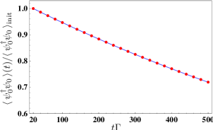
Figure 3: (Color online) Decay of the $k=0$ polariton mode for non-degenerate ground states $|1\rangle$ and $|2\rangle$. The solid line shows the decay according to Eq. (62), the corresponding result from a numerical integration of Maxwell-Bloch equations is indicated by red dots. The parameters are $\Delta\omega=150\Gamma$, $\cos^{2}\theta=2.5\times 10^{-4}$, $\Omega_{0}=90\Gamma$, $\delta=0$ and $\varepsilon$ is fixed by Eq. (37). The initial spin coherence $R_{21}$ (see Appendix D) has a Gaussian shape $R_{21}\propto\exp[-(z-z_{0})^{2}/(2\sigma^{2})]$ with $\sigma=24.3\Gamma c/\Omega_{0}^{2}$, and the control fields are ramped up according to $\Omega_{c}(t)=0.5[1+\tanh(t-10/\Gamma)]\times\Gamma$. The initial value $\langle\psi_{0}^{\dagger}\psi_{0}\rangle_{\text{init}}$ refers to $\langle\psi_{0}^{\dagger}\psi_{0}\rangle$ at $t=20/\Gamma$ where the control fields have attained their maximal value of $\Omega_{c}=\Gamma$.

The term $\mathcal{L}_{1}\varrho_{\text{D}}$ arises due to the coupling between dark-state polaritons and the difference mode $D_{k}$. Since the decay rate of the individual modes increases quadratically with the wave number, $\mathcal{L}_{1}\varrho_{\text{D}}$ does not result in an exponential damping but leads to diffusion Bajcsy et al. (2003); Zimmer et al. (2006). On the contrary, $\mathcal{L}_{2}\varrho_{\text{D}}$ leads to identical decay rates for all modes. This term stems from the coupling between dark-state polaritons $\psi_{k}$ and bright polaritons $\phi_{k}$. Since this loss mechanism has not been discussed in the literature yet, we investigate it in more detail here. First of all, we note that $\mathcal{L}_{2}\varrho_{\text{D}}$ is proportional to $\Delta\omega^{2}$, and $\Delta\omega$ practically coincides with the splitting of the ground states $|1\rangle$ and $|2\rangle$ [see Eq. (9)]. An important consequence of $\mathcal{L}_{2}\varrho_{\text{D}}$ is that in contrast to EIT, dark-state polaritons in the $k=0$ mode decay under the conditions of stationary light provided that the ground states $|1\rangle$ and $|2\rangle$ are non-degenerate. The decay of the mean number of dark-state polaritons in the $k=0$ mode can be calculated from Eq. (56) and is given by

$$\partial_{t}\langle\psi_{0}^{\dagger}\psi_{0}\rangle=-\frac{\Gamma}{\Omega_{0}^{2}}\Delta\omega^{2}\cos^{2}\theta\langle\psi_{0}^{\dagger}\psi_{0}\rangle.$$ (62)

The accuracy of this result can be confirmed numerically if $\langle\psi_{0}^{\dagger}\psi_{0}\rangle$ is evaluated via Maxwell-Bloch equations for classical probe fields (see Appendix D). The result is shown in Fig. 3, where the solid line corresponds to the exponential decay according to Eq. (62). The dotted line represents $\langle\psi_{0}^{\dagger}\psi_{0}\rangle$ obtained from the numerical integration of Maxwell-Bloch equations and is in perfect agreement with the predictions of the master equation (56).

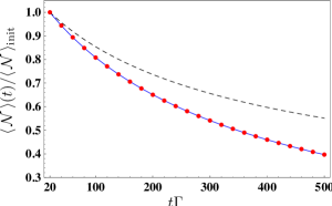
Figure 4: (Color online) The number of dark-state polaritons is shown as a function of time. The results of Eqs. (64) and Eq. (65) are represented by the solid and the dotted line, respectively. The good agreement indicates that the polariton losses are described correctly by the master equation (56). The number of polaritons follows the dashed line if the additional decay term $\mathcal{L}_{2}\varrho_{\text{D}}$ in Eq. (56) is omitted. The parameters are the same as in Fig. 3.

Next we compare the impact of the loss terms $\mathcal{L}_{1}\varrho_{\text{D}}$ and $\mathcal{L}_{2}\varrho_{\text{D}}$. Equations (59) and (60) imply that $\mathcal{L}_{2}\varrho_{\text{D}}$ becomes comparable to $\mathcal{L}_{1}\varrho_{\text{D}}$ if $|\Delta\omega|$ is of the order of $ck_{\text{max}}$. Since $ck_{\text{max}}\approx|\Delta\omega|+c\sigma_{k}$ where $\sigma_{k}$ is the width of the polariton pulse in $k$ space, the two loss terms are comparable if

$$|\Delta\omega|\geq c\sigma_{k}.$$ (63)

On the other hand, the width $\sigma_{k}$ can be estimated to be of the order of $2\pi/L$, where $L$ is the length of the system. The inequality (63) thus implies that the impact of $\mathcal{L}_{2}\varrho_{\text{D}}$ is of the same order of $\mathcal{L}_{1}\varrho_{\text{D}}$ if the wavelength associated with the beat note $\Delta\omega$ of the probe and control fields is comparable or shorter than $L$. For realistic values of $L$ of a few centimeters, the term $\mathcal{L}_{2}\varrho_{\text{D}}$ will have a significant impact if $|\Delta\omega|$ is of the order of a few GHz or larger. Note that polariton losses can be minimized by minimizing $|\Delta\omega|$. This is obvious for $\mathcal{L}_{2}\varrho_{\text{D}}$ since it is proportional to $\Delta\omega^{2}$. However, also the impact of $\mathcal{L}_{1}\varrho_{\text{D}}$ increases with increasing values of $|\Delta\omega|$ since $ck_{\text{max}}\approx|\Delta\omega|+c\sigma_{k}$.

The total losses of dark-state polaritons can be calculated from Eq. (56). We find that the mean number of dark-state polaritons $\langle\mathcal{N}\rangle$ obeys

$$\partial_{t}\langle\mathcal{N}\rangle=-\frac{\Gamma}{\Omega_{0}^{2}}\cos^{2}\theta\left(\Delta\omega^{2}+\frac{1}{\langle\mathcal{N}\rangle}\sum\limits_{k}\omega_{k}^{2}\langle\psi_{k}^{\dagger}\psi_{k}\rangle\right)\langle\mathcal{N}\rangle,$$ (64)

where $\mathcal{N}=\sum_{k}\psi_{k}^{\dagger}\psi_{k}$ is the polariton number operator. The solid line in Fig. 4 shows the losses of polaritons according to Eq. (64) where $\langle\psi_{k}^{\dagger}\psi_{k}\rangle$ was calculated via the numerical integration of Maxwell-Bloch equations, see Appendix D. On the other hand, the number of dark-state polaritons is proportional to the electromagnetic field intensity,

$$\langle\mathcal{N}\rangle\propto\int\limits_{0}^{L}\text{d}z\left(|\mathcal{G}_{+}|^{2}+|\mathcal{G}_{-}|^{2}\right),$$ (65)

where $\mathcal{G}_{+}$ ($\mathcal{G}_{-}$) is the Rabi frequency of the classical probe field propagating in the positive (negative) $z$ direction. In order to test Eq. (64), we evaluate the right-hand side of Eq. (65) as a function of time from a numerical integration of Maxwell-Bloch equations. The result is shown as the dotted line in Fig. 4 and in excellent agreement with the findings of Eq. (64). Finally, the dashed line in Fig. 4 represents the polariton losses if the term $\mathcal{L}_{2}\varrho_{\text{D}}$ were neglected and shows that $\mathcal{L}_{2}\varrho_{\text{D}}$ contributes significantly. Note that the parameters of the first stationary light experiment Bajcsy et al. (2003) indicate a ratio of $|\Delta\omega|/(ck_{\text{max}})\approx 0.75$, which is even larger than the value of $|\Delta\omega/(ck_{\text{max}})\approx 0.25$ chosen in Fig. 4.

We emphasize that the loss term $\mathcal{L}_{2}\varrho_{\text{D}}$ arises only in the presence of two counter-propagating control fields. In this case, the photonic component $A_{k}$ in Eq. (14) of the dark-state polaritons $\psi_{k}$ is comprised of counter-propagating probe field modes that are grouped around the wave numbers $\pm k_{c}$ of the control field rather than the probe field, see Sec. III.2. It follows that the total Hamiltonian $H=H_{0}+H_{\Lambda}+H_{\text{NL}}$ in Sec. II does not possess a true dark state for $\Delta\omega\not=0$. Even the dark-state polaritons $\psi_{k}$ in the $k=0$ mode experience a coupling to bright-state polaritons $\phi_{k}$ and thus decay. This mechanism is at the heart of Eq. (62) that describes the loss of dark-state polaritons in the $k=0$ mode. The situation is different in a standard EIT configuration where only one pair of co-propagating probe and control fields is present, and the loss of dark-state polaritons is described by $\mathcal{L}_{1}\varrho_{\text{D}}$ only.

IV.2 STATIONARY LIGHT WITH TWO-PARTICLE INTERACTION

Next we restate the full master equation (45) in terms of the field operators $\psi(z)$ defined in Eq. (54). In addition to the terms discussed in Sec. IV.1, we have to take into account all contributions proportional to the coupling constant $g_{2}$ in Eq. (45) that account for elastic and inelastic polariton-polariton interactions. We obtain Kiffner and Hartmann (2010)

$$\hbar\dot{\varrho_{\text{D}}}=-iH_{\text{eff}}\varrho_{\text{D}}+i\varrho_{\text{D}}H_{\text{eff}}^{\dagger}+\mathcal{I}\varrho_{\text{D}}+\hbar\mathcal{L}_{1}\varrho_{\text{D}}+\hbar\mathcal{L}_{2}\varrho_{\text{D}},$$ (66)

where $H_{\text{eff}}$ is a non-hermitian Hamiltonian,

$$H_{\text{eff}}=H_{3}+\frac{\tilde{g}}{2}\int_{0}^{L}\text{d}z\psi^{\dagger 2}\psi^{2}\,,$$ (67)

and $H_{3}$, $\mathcal{L}_{1}\varrho_{\text{D}}$ and $\mathcal{L}_{2}\varrho_{\text{D}}$ are defined in Eqs. (57), (59) and (60), respectively. The parameter

$$\tilde{g}=\frac{2\hbar Lg_{2}^{2}\cos^{2}\theta}{\Delta-\cos^{2}\theta\Delta\omega+i\gamma_{42}/2}$$ (68)

is the complex coupling constant, and

$$\mathcal{I}\varrho_{\text{D}}=-\text{Im}(\tilde{g})\int\limits_{0}^{L}\text{d}z\psi^{2}\varrho_{\text{D}}\psi^{\dagger 2}.$$ (69)

The term proportional to $\tilde{g}$ in Eq. (67) and $\mathcal{I}\varrho_{\text{D}}$ in Eq. (69) account for elastic and inelastic two-particle interactions that originate from the coupling of dark-state polaritons to the excited state $|4\rangle$. More precisely, the real part of $\tilde{g}$ gives rise to a hermitian contribution to $H_{\text{eff}}$ that accounts for elastic two-particle collisions. On the other hand, the imaginary part of $\tilde{g}$ together with $\mathcal{I}\varrho_{\text{D}}$ gives rise to a two-particle loss term that can be written in Lindblad form as $\text{Im}(\tilde{g}/2)\mathcal{D}[\psi^{2}]$.

The master equation (66) is equivalent to Eq. (45) and describes a one-dimensional system of bosons with effective mass $m_{\text{eff}}$ that experience elastic and inelastic two-particle interactions. Except for the two loss terms $\mathcal{L}_{1}\varrho_{\text{D}}$ and $\mathcal{L}_{2}\varrho_{\text{D}}$, Eq. (66) can be identified with the dissipative Lieb-Liniger model discussed in the next Section.

IV.3 DISSIPATIVE LIEB-LINIGER MODEL

The original Lieb-Liniger model Lieb and Liniger (1963) established in 1963 describes bosons in one dimension that experience a repulsive contact interaction. In the limit of strong interactions, the bosons can enter the regime of a Tonks-Girardeau gas Girardeau (1960) where they behave with respect to many observables as if they were fermions. Recently, it was shown Dürr et al. (2009) that the original Lieb-Liniger model can be generalized to systems where the bosons experience a contact interaction with complex coupling constant, i.e., they undergo elastic or inelastic two-particle interactions. This dissipative Lieb-Liniger model Dürr et al. (2009) shows that even a purely dissipative interaction effectively results in a repulsion and produces a Tonks-Girardeau gas in the limit of strong interactions.

The master equation (66) can be identified with the dissipative Lieb-Liniger model provided that the loss terms $\mathcal{L}_{1}\varrho_{\text{D}}$ and $\mathcal{L}_{2}\varrho_{\text{D}}$ are negligible. In the following we specify the conditions that justify this approximation and assume that $\Delta\omega^{2}$ is small enough such that the impact of $\mathcal{L}_{2}\varrho_{\text{D}}$ is small as compared to $\mathcal{L}_{1}\varrho_{\text{D}}$, see Section IV.1. On the other hand, the diffusion term $\mathcal{L}_{1}\varrho_{\text{D}}$ is negligible if two conditions are met. First, the dynamics induced by the kinetic energy term proportional to $m_{\text{eff}}$ in Eq. (67) must be fast as compared to the inverse decay rate of polaritons introduced by $\mathcal{L}_{1}\varrho_{\text{D}}$. This can be achieved if we set $|\delta|\gg\Gamma$. Second, losses due to $\mathcal{L}_{1}\varrho_{\text{D}}$ must be negligible which imposes a limit on the maximal evolution time

$$t_{\text{max}}\ll\frac{1}{\Gamma}\frac{1}{\cos^{2}\theta}\frac{2\Omega_{0}^{2}}{c^{2}k_{\text{max}}^{2}}.$$ (70)

Note that $t_{\text{max}}\gg 1/\Gamma$ is much larger than the lifetime of the excited state $|3\rangle$. Under these conditions, the master equation (66) reduces to

$$\hbar\dot{\varrho_{\text{D}}}=-iH_{\text{eff}}\varrho_{\text{D}}+i\varrho_{\text{D}}H_{\text{eff}}^{\dagger}+\mathcal{I}\varrho_{\text{D}}$$ (71)

and can be identified with the generalized Lieb-Liniger model Dürr et al. (2009) for a one-dimensional system of bosons with mass $m_{\text{eff}}$ and complex interaction parameter $\tilde{g}$. All features of the Lieb-Liniger model Lieb and Liniger (1963); Dürr et al. (2009) are characterized by a single, dimensionless parameter

$$G=\frac{m_{\text{eff}}\tilde{g}}{\hbar^{2}N_{\text{ph}}/L},$$ (72)

where $N_{\text{ph}}$ is the number of photons in the pulse. In the strongly correlated regime $|G|\gg 1$, the interaction between the particles creates a Tonks-Girardeau (TG) gas where polaritons behave like impenetrable hard-core particles that never occupy the same position. Depending on the sign of the detuning $\delta$ and $\Delta$, the elastic interaction between the polaritons can be either attractive or repulsive. The dissipative component of the interaction is negligible for $\Delta\gg\gamma_{42}$. In this case, the preparation of a TG gas of polaritons with repulsion can be achieved if $\delta\Delta<0$ Chang et al. (2008). Note that the interaction becomes attractive if $\delta\Delta>0$ which opens up the possibility to enter the super Tonks-Girardeau regime for polaritons Astrakharchik et al. (2005); Batchelor et al. (2005); Haller et al. (2009). Since the coupling constant $\tilde{g}$ in Eq. (68) is maximal for $\Delta=0$, the Lieb-Liniger parameter $|G|$ and hence the induced correlations are maximal for purely dissipative interactions Kiffner and Hartmann (2010).

IV.4 OTHER REALIZATIONS

The master equation for dark-state polaritons in Sec. IV was derived under the assumption that the level scheme of each atom is given by Fig. 2. Here we point out that stationary light and interacting dark-state polaritons can be realized as well with the level scheme in Fig. 5 that was suggested in Zimmer et al. (2008); Fleischhauer et al. (2008). Moreover, a straightforward modification of the formalism described in Sec. III demonstrates that the level scheme of Fig. 5 leads to the same master equation (45) for dark-state polaritons as the configuration in Fig. 2. On the contrary, each system displays characteristic advantages and disadvantages that we discuss now.

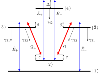
Figure 5: (Color online) Alternative level scheme that gives rise to the master equation for polaritons described in Sec. IV. All symbols are defined in the same way as in Fig. 2.

The major difference between the two configurations is that the level scheme in Fig. 5 creates stationary light via the double-$\Lambda$ system formed by states $|1\rangle$, $|2\rangle$, $|3\rangle$ and $|\tilde{3}\rangle$. Here each probe field interacts only with the co-propagating control field, and thus no fast oscillating spin coherences $X_{k}(m)$ for $m\not=0$ are produced com (a). This feature is a significant advantage of the system shown in Fig. 5, since it implies that the master equation (45) remains valid for ultracold atoms or stationary atoms where the condition (53) cannot be fulfilled.

On the other hand, the implementation of the configuration in Fig. 5 comes along with difficulties that do not occur in the case of the level scheme in Fig. 2. First, we note that the transitions in the $\Lambda$ configuration of Fig. 2 can be selected by polarization, even if the ground states $|1\rangle$ and $|2\rangle$ are degenerate. This is not the case for the level scheme in Fig. 5 where the level splitting between the ground states $|1\rangle$ and $|2\rangle$ must be large enough such that the transitions $|2\rangle\leftrightarrow|3\rangle$, $|1\rangle\leftrightarrow|3\rangle$ and $|2\rangle\leftrightarrow|\tilde{3}\rangle$, $|1\rangle\leftrightarrow|\tilde{3}\rangle$ can be addressed independently. Consequently, the parameter $|\Delta\omega|$ must be significantly larger than the Rabi frequencies $\Omega_{\pm}$ of the control fields which leads to additional losses, see Sec. IV. Second, we point out that the initial polariton pulse in $k$ space is centered around $\Delta\omega/c$ if it is prepared via the slowing and stopping of a probe pulse. The reason for this is that the wave numbers $k$ of stationary-light polaritons have to be grouped around the wavenumbers $\pm k_{c}$ of the control fields, see Sec. III.2. If the kinetic energy of the stationary-light polaritons is different from zero (i.e., $\delta\not=0$) and in the case of the level scheme of Fig. 5, the mandatory choice of $\Delta\omega\not=0$ will lead to a moving polariton pulse even if the control fields have the same intensity.

V SUMMARY

In this paper we introduced a technique for the description of light-matter interactions under conditions of EIT. More specifically, we described a general method for the derivation of a master equation for dark-state polaritons. In contrast to the standard description Fleischhauer and Lukin (2000, 2002) based on a Heisenberg-Langevin approach, our master equation facilitates the treatment of polariton losses. This achievement allows us to model general polariton-polariton interactions that may be conservative, dissipative or a mixture of both. In particular, the master equation approach enables us to study dissipation-induced correlations Syassen et al. (2008); Dürr et al. (2009) that are promising in the quest for highly correlated systems since they can be considerably stronger than their conservative counterparts Kiffner and Hartmann (2010). For the illustration of our technique we use the example of stationary light polaritons that experience a conservative or dissipative interaction. The resulting master equation is discussed in various limiting cases. For stationary-light polaritons we find an additional loss mechanism that was overlooked so far. It is related to the fact that the total Hamiltonian of the system does not possess a true dark state if the ground states are non-degenerate. In particular, polariton losses in level configurations with non-degenerate ground states can be a multiple of those in level schemes with degenerate ground states. Furthermore, we specified conditions that allow us to reduce the full master equation for dark-state polaritons to the dissipative Lieb-Liniger model Dürr et al. (2009). Finally, we discussed the atomic level scheme in Fig. 5 that leads to the same master equation for dark-state polaritons as the one in Fig. 2 and compared the advantages and disadvantages of both configurations.

At the heart of our approach is a mapping of the full system dynamics to a conceptually simple system of coupled bosonic modes. This mapping could be the starting point for future studies of EIT systems beyond a Markovian master equation for dark-state polaritons.

Appendix A REPRESENTATION OF OPERATORS IN $\mathcal{H}_{\text{FE}}$

Here we show how the master equation Eq. (2) can be expressed in terms of bosonic creation and annihilation operators if the system dynamics is restricted to the subspace $\mathcal{H}_{\text{FE}}$. To this end, let $\hat{X}$ be an operator acting on the total state space $\mathcal{H}_{\text{tot}}$. In the following, we describe a procedure that allows one to construct an operator $\hat{X}_{O}$ that comprises of bosonic operators $O_{i}\in\mathcal{O}$ [see Eq. (23)] and that coincides approximately with $\hat{X}$ in the subspace $\mathcal{H}_{\text{FE}}$. The latter condition implies that $\hat{X}_{O}$ and $\hat{X}$ must necessarily obey the same commutation relations with the creation operators $O_{i}^{\dagger}$ ($O_{i}\in\mathcal{O}$) in $\mathcal{H}_{\text{FE}}$,

$$\left[\hat{X},O_{i}^{\dagger}\right]_{\mathcal{H}_{\text{FE}}}=\left[\hat{X}_{O},O_{i}^{\dagger}\right]_{\mathcal{H}_{\text{FE}}}.$$ (73)

Furthermore, we have $\hat{X}_{O}|s\rangle=\hat{X}|s\rangle$ for an arbitrary state $|s\rangle\in\mathcal{H}_{\text{FE}}$. In all situations considered below, the operator $\hat{X}$ annihilates the vacuum state, $\hat{X}|0\rangle=0$. In addition to Eq. (73), we thus require

$$\hat{X}_{O}|0\rangle=0\,.$$ (74)

The two conditions in Eqs. (73) and (74) are sufficient to determine $\hat{X}_{O}$ since they guarantee that the matrix elements of $\hat{X}$ and $\hat{X}_{O}$ are identical in the subspace $\mathcal{H}_{\text{FE}}$. In order to see this, we evaluate the action of $\hat{X}$ applied to the states $|\{n_{1},\ldots,n_{M}\}\rangle$ that span $\mathcal{H}_{\text{FE}}$,

$$\hat{X}|\{n_{1},\ldots,n_{M}\}\rangle=\left[\hat{X},\prod_{i=1}^{M}\frac{1}{\sqrt{n_{i}!}}\big{(}\hat{O}_{i}^{\dagger}\big{)}^{n_{i}}\right]|0\rangle\,.$$ (75)

Here we employed the definition (11) and the relation $\hat{X}|0\rangle=0$. The recursive application of the identity $[A,BC]=[A,B]C+B[A,C]$ allows us to write the commutator on the right-hand side of Eq. (75) as a sum of terms where only the commutator of $\hat{X}$ with one of the creation operators $O_{i}^{\dagger}$ appears. Therefore, Eqs. (73) and (74) guarantee that the matrix elements of $\hat{X}$ and $\hat{X}_{O}$ are identical in the subspace $\mathcal{H}_{\text{FE}}$.

As an example, we discuss the representation of $\sum_{\mu=1}^{N}A_{22}^{(\mu)}$ in terms of the operators $O_{i}\in\mathcal{O}$. The only non-vanishing commutators are

$$\left[\sum\limits_{\mu=1}^{N}A_{22}^{(\mu)},X_{k}^{\dagger}(m)\right]=X_{k}^{\dagger}(m),$$ (76)

and we have $\sum_{\mu=1}^{N}A_{22}^{(\mu)}|0\rangle=0$. According to Eqs. (73), (74) and with the bosonic commutation relations obeyed by the operators $X_{k}(m)$, the representation of $\sum_{\mu=1}^{N}A_{22}^{(\mu)}$ in $\mathcal{H}_{\text{FE}}$ is given by

$$\sum\limits_{\mu=1}^{N}A_{22}^{(\mu)}=\sum\limits_{m}\sum\limits_{k}X_{k}^{\dagger}(m)X_{k}(m).$$ (77)

The representation of the remaining operators that appear in the Hamiltonian $H$ in Eq. (2) can be found in a similar way, the result is

$$\sum\limits_{\mu=1}^{N}A_{33}^{(\mu)}=\sum\limits_{m}\sum\limits_{k}H_{k}^{\dagger}(m)H_{k}(m),$$ (78)

$$\sum\limits_{\mu=1}^{N}A_{44}^{(\mu)}=\sum\limits_{m}\sum\limits_{k}I_{k}^{\dagger}(m)I_{k}(m),$$ (79)

$$\sum\limits_{\mu=1}^{N}S_{32}^{(\mu)}e^{ik_{c}z_{\mu}}=\sum\limits_{m}\sum\limits_{k}X_{k}(m)H_{k}^{\dagger}(m+1),$$ (80)

$$\sum\limits_{\mu=1}^{N}S_{32}^{(\mu)}e^{-ik_{c}z_{\mu}}=\sum\limits_{m}\sum\limits_{k}X_{k}(m)H_{k}^{\dagger}(m-1),$$ (81)

$$\sum\limits_{\mu=1}^{N}S_{42}^{(\mu)}e^{i(k_{c}+k)z_{\mu}}=\sum\limits_{m}\sum\limits_{p}X_{p-k}(m)I_{p}^{\dagger}(m+1),$$ (82)

$$\sum\limits_{\mu=1}^{N}S_{42}^{(\mu)}e^{-i(k_{c}-k)z_{\mu}}=\sum\limits_{m}\sum\limits_{p}X_{p-k}(m)I_{p}^{\dagger}(m-1).$$ (83)

These relations together with the inverse relations of Eqs. (14) and (15) allow us to find the representation of $H_{0}$, $H_{\Lambda}$ and $H_{\text{NL}}$ in $\mathcal{H}_{\text{FE}}$,

$$\tilde{H}_{0}= -\hbar\Delta\omega\sum_{k}\left(A_{k}^{\dagger}A_{k}+D_{k}^{\dagger}D_{k}\right)+2\hbar\sin\varphi\cos\varphi\sum_{k}\omega_{k}\left(A_{k}^{\dagger}D_{k}+A_{k}D_{k}^{\dagger}\right)$$ (84)

$$-\hbar\varepsilon\sum\limits_{m}\sum\limits_{k}X_{k}^{\dagger}(m)X_{k}(m)-\hbar\delta\sum\limits_{m}\sum\limits_{k}H_{k}^{\dagger}(m)H_{k}(m)-\hbar(\Delta+\varepsilon)\sum\limits_{m}\sum\limits_{k}I_{k}^{\dagger}(m)I_{k}(m)$$ (85)

$$-\hbar(\sin^{2}\varphi-\cos^{2}\varphi)\sum_{k}\omega_{k}\left(D_{k}^{\dagger}D_{k}-A_{k}^{\dagger}A_{k}\right),$$

$$\tilde{H}_{\Lambda}= -\hbar\Omega_{0}\sin\theta\sum\limits_{k}\left\{A_{k}\left[H_{k}^{\dagger}(1)\sin\varphi+H_{k}^{\dagger}(-1)\cos\varphi\right]+D_{k}\left[H_{k}^{\dagger}(1)\cos\varphi-H_{k}^{\dagger}(-1)\sin\varphi\right]\right\}$$ (86)

$$-\hbar\Omega_{0}\cos\theta\sum\limits_{m}\sum\limits_{k}X_{k}(m)\left[H_{k}^{\dagger}(m+1)\sin\varphi+H_{k}^{\dagger}(m-1)\cos\varphi\right]+\text{h.c.},$$

$$\tilde{H}_{\text{NL}}= -\hbar g_{2}\sum\limits_{k}A_{k}\sum\limits_{m}\sum\limits_{p}X_{p-k}(m)\left[I_{p}^{\dagger}(m+1)\sin\varphi+I_{p}^{\dagger}(m-1)\cos\varphi\right]$$ (87)

$$-\hbar g_{2}\sum\limits_{k}D_{k}\sum\limits_{m}\sum\limits_{p}X_{p-k}(m)\left[I_{p}^{\dagger}(m+1)\cos\varphi-I_{p}^{\dagger}(m-1)\sin\varphi\right]+\text{h.c.}.$$

For the full representation of the master equation in $\mathcal{H}_{\text{FE}}$ it remains to transform the decay term $\mathcal{L}_{\gamma}\varrho_{\text{D}}$, see Eq. (8). The representation of the terms that describe the decay of the excited states in Eq. (8) can be found via Eqs. (78) and (79). Since the super-operator $\tilde{\mathcal{L}}_{\gamma}\tilde{\varrho}$ must preserve the trace of the density operator, we find

$$\tilde{\mathcal{L}}_{\gamma}\tilde{\varrho}= -\frac{\Gamma}{2}\sum\limits_{m}\sum\limits_{k}\left[H_{k}^{\dagger}(m)H_{k}(m)\tilde{\varrho}+\tilde{\varrho}H_{k}^{\dagger}(m)H_{k}(m)-2H_{k}(m)\tilde{\varrho}H_{k}^{\dagger}(m)\right]$$ (88)

$$-\frac{\gamma_{42}}{2}\sum\limits_{m}\sum\limits_{k}\left[I_{k}^{\dagger}(m)I_{k}(m)\tilde{\varrho}+\tilde{\varrho}I_{k}^{\dagger}(m)I_{k}(m)-2I_{k}(m)\tilde{\varrho}I_{k}^{\dagger}(m)\right],$$

where $\Gamma=\gamma_{31}+\gamma_{32}$ is the full decay rate of the excited state $|3\rangle$.

Appendix B DEFINITIONS

The master equation (35) is obtained from (25) for $\Omega_{+}=\Omega_{-}$ and if we exchange the set of operators $\{A_{k},X_{k}(0),H_{k}(1),H_{k}(-1),I_{k}(1),I_{k}(-1)\}$ by the new set $\{\psi_{k},\phi_{k},P_{k},Q_{k},U_{k},V_{k}\}$ according to

$$\psi_{k}=A_{k}\cos\theta-X_{k}(0)\sin\theta, \phi_{k}=A_{k}\sin\theta+X_{k}(0)\cos\theta,$$ (89)

$$P_{k}=[H_{k}(1)+H_{k}(-1)]/\sqrt{2}, Q_{k}=[H_{k}(1)-H_{k}(-1)]/\sqrt{2},$$ (90)

$$U_{k}=[I_{k}(1)+I_{k}(-1)]/\sqrt{2}, V_{k}=[I_{k}(1)-I_{k}(-1)]/\sqrt{2}.$$ (91)

Since the old and new operators are related by a unitary transformation, the new operators $\{\psi_{k},\phi_{k},P_{k},Q_{k},U_{k},V_{k}\}$ obey bosonic commutation relations. If the inverse relations of Eqs. (89)-(91) are plugged into Eqs. (84), (86)  (87) and (88), we obtain the master equation (35). Furthermore, we employ the condition in Eq. (37) and the definition $\Delta_{\theta}=\Delta-\cot^{2}\theta\Delta\omega$. The bath Hamiltonian in Eq. (38) is comprised of four parts,

$$H_{\text{B}}=H_{\text{B}}^{(0)}+H_{\text{B}}^{(1)}+H_{\text{B}}^{(2)}+H_{\text{B}}^{(3)},\qquad\text{where}$$ (92)

$$H_{\text{B}}^{(0)}= -\hbar\Delta\omega\sum\limits_{k}\left(D_{k}^{\dagger}D_{k}+\phi_{k}^{\dagger}\phi_{k}\right)-\hbar\delta\sum\limits_{k}\left(P_{k}^{\dagger}P_{k}+Q_{k}^{\dagger}Q_{k}\right)-\hbar\Delta_{\theta}\sum\limits_{k}\left(U_{k}^{\dagger}U_{k}+V_{k}^{\dagger}V_{k}\right)$$ (93)

$$+\hbar\sum\limits_{k}\omega_{k}\left(\phi_{k}^{\dagger}D_{k}+D_{k}^{\dagger}\phi_{k}\right)-\hbar\Omega_{0}\sum\limits_{k}\left(P_{k}^{\dagger}\phi_{k}+P_{k}\phi_{k}^{\dagger}+Q_{k}^{\dagger}D_{k}+D_{k}^{\dagger}Q_{k}\right)$$

$$-\hbar\varepsilon\sum\limits_{\genfrac{}{}{0.0pt}{2}{m}{m\not=0}}\sum\limits_{k}X_{k}^{\dagger}(m)X_{k}(m)-\hbar\delta\sum\limits_{\genfrac{}{}{0.0pt}{2}{m}{m\not=0}}\sum\limits_{k}H_{k}^{\dagger}(m)H_{k}(m)-\hbar\Delta_{\theta}\sum\limits_{\genfrac{}{}{0.0pt}{2}{m}{m\not=0}}\sum\limits_{k}I_{k}^{\dagger}(m)I_{k}(m),$$

$$H_{\text{B}}^{(1)}= -\frac{1}{2}\hbar\Omega_{0}\cos\theta\sum\limits_{k}\left[X_{k}(-2)\left(P_{k}^{\dagger}-Q_{k}^{\dagger}\right)+X_{k}(2)\left(P_{k}^{\dagger}+Q_{k}^{\dagger}\right)\right]$$ (94)

$$-\frac{1}{\sqrt{2}}\hbar\Omega_{0}\cos\theta\sum\limits_{k}\Big{[}\sum\limits_{\genfrac{}{}{0.0pt}{2}{m}{m\not=0,-2}}X_{k}(m)H_{k}^{\dagger}(m+1)+\sum\limits_{\genfrac{}{}{0.0pt}{2}{m}{m\not=0,2}}X_{k}(m)H_{k}^{\dagger}(m-1)\Big{]}+\text{h.c.},$$

$$H_{\text{B}}^{(2)}= -\hbar g_{2}\cos\theta\sum\limits_{k}\Big{[}U_{k}^{\dagger}\sum\limits_{p}\phi_{p}\phi_{k-p}+V_{k}^{\dagger}\sum\limits_{p}D_{p}\phi_{k-p}\Big{]}+\text{h.c.},$$ (95)

$$H_{\text{B}}^{(3)}= -\frac{1}{2}\hbar g_{2}\sum\limits_{k}\sum\limits_{p}\left[\left(U_{k}^{\dagger}-V_{k}^{\dagger}\right)X_{k-p}(-2)\left(\phi_{p}+D_{p}\right)+\left(U_{k}^{\dagger}+V_{k}^{\dagger}\right)X_{k-p}(2)\left(\phi_{p}-D_{p}\right)\right]$$ (96)

$$-\frac{1}{\sqrt{2}}\hbar g_{2}\sum\limits_{k}\sum\limits_{p}\Big{[}\sum\limits_{\genfrac{}{}{0.0pt}{2}{m}{m\not=0,-2}}I_{k}^{\dagger}(m+1)X_{k-p}(m)(\phi_{p}+D_{p})+\sum\limits_{\genfrac{}{}{0.0pt}{2}{m}{m\not=0,2}}I_{k}^{\dagger}(m-1)X_{k-p}(m)(\phi_{p}-D_{p})\Big{]}+\text{h.c.}.$$

The dominant contribution to the bath Hamiltonian $H_{\text{B}}$ is represented by $H_{\text{B}}^{(0)}$. The term $H_{\text{B}}^{(1)}$ accounts for the modification of stationary light due to the fast oscillating spin coherences. Furthermore, $H_{\text{B}}^{(2)}$ and $H_{\text{B}}^{(3)}$ arise from the coupling of bath excitations to the transition $|4\rangle\leftrightarrow|2\rangle$. We write the interaction Hamiltonian in Eq. (38) as a sum of three parts

$$V=V^{(0)}+V^{(1)}+V^{(2)},\qquad\text{where}$$ (97)

$$V^{(0)}= -\hbar\cos\theta\Delta\omega\sum\limits_{k}\left(\psi_{k}^{\dagger}\phi_{k}+\psi_{k}\phi_{k}^{\dagger}\right)+\hbar\cos\theta\sum\limits_{k}\omega_{k}\left(\psi_{k}^{\dagger}D_{k}+D_{k}^{\dagger}\psi_{k}\right)$$ (98)

$$+\hbar g_{2}\cos\theta\sum\limits_{k}\left(U_{k}^{\dagger}\sum\limits_{p}\psi_{p}\psi_{k-p}+U_{k}\sum\limits_{p}\psi_{p}^{\dagger}\psi_{k-p}^{\dagger}\right),$$

$$V^{(1)}= \hbar g_{2}\sum\limits_{k}\Big{(}U_{k}^{\dagger}\sum\limits_{p}\phi_{p}\psi_{k-p}+V_{k}^{\dagger}\sum\limits_{p}D_{p}\psi_{k-p}\Big{)}+\text{h.c.},$$ (99)

$$V^{(2)}= -\frac{1}{2}\hbar g_{2}\cos\theta\sum\limits_{k}\sum\limits_{p}\left[\left(U_{k}^{\dagger}-V_{k}^{\dagger}\right)\psi_{p}X_{k-p}(-2)+\left(U_{k}^{\dagger}+V_{k}^{\dagger}\right)\psi_{p}X_{k-p}(2)\right]$$ (100)

$$-\frac{1}{\sqrt{2}}\hbar g_{2}\cos\theta\sum\limits_{k}\sum\limits_{p}\Big{[}\sum\limits_{\genfrac{}{}{0.0pt}{2}{m}{m\not=0,-2}}I_{k}^{\dagger}(m+1)\psi_{p}X_{k-p}(m)+\sum\limits_{\genfrac{}{}{0.0pt}{2}{m}{m\not=0,2}}I_{k}^{\dagger}(m-1)\psi_{p}X_{k-p}(m)\Big{]}+\text{h.c.}.$$ (101)

The term $V^{(0)}$ describes the coupling of one or two dark-state polaritons to one bath excitation. On the other hand, $V^{(1)}$ arises from the coupling of one dark-state polariton and one bath excitation to the transition $|4\rangle\leftrightarrow|2\rangle$. The remaining part $V^{(2)}$ accounts for the coupling of a dark-state polariton and a fast spin coherence to the transition $|4\rangle\leftrightarrow|2\rangle$. Finally, the decay term $\mathcal{L}_{\gamma}^{(\text{B})}\tilde{\varrho}$ in Eq. (38) reads

$$\mathcal{L}_{\gamma}^{(\text{B})}\tilde{\varrho}= -\frac{\Gamma}{2}\sum\limits_{k}\left(P_{k}^{\dagger}P_{k}\tilde{\varrho}+\tilde{\varrho}P_{k}^{\dagger}P_{k}-2P_{k}\tilde{\varrho}P_{k}^{\dagger}\right)-\frac{\Gamma}{2}\sum\limits_{k}\left(Q_{k}^{\dagger}Q_{k}\tilde{\varrho}+\tilde{\varrho}Q_{k}^{\dagger}Q_{k}-2Q_{k}\tilde{\varrho}Q_{k}^{\dagger}\right)$$ (102)

$$-\frac{\Gamma}{2}\sum\limits_{\genfrac{}{}{0.0pt}{2}{m}{m\not=\pm 1}}\sum\limits_{k}\left[H_{k}^{\dagger}(m)H_{k}(m)\tilde{\varrho}+\tilde{\varrho}H_{k}^{\dagger}(m)H_{k}(m)-2H_{k}(m)\tilde{\varrho}H_{k}^{\dagger}(m)\right]$$

$$-\frac{\gamma_{42}}{2}\sum\limits_{k}\left(U_{k}^{\dagger}U_{k}\tilde{\varrho}+\tilde{\varrho}U_{k}^{\dagger}U_{k}-2U_{k}\tilde{\varrho}U_{k}^{\dagger}\right)-\frac{\gamma_{42}}{2}\sum\limits_{k}\left(V_{k}^{\dagger}V_{k}\tilde{\varrho}+\tilde{\varrho}V_{k}^{\dagger}V_{k}-2V_{k}\tilde{\varrho}V_{k}^{\dagger}\right)$$

$$-\frac{\gamma_{42}}{2}\sum\limits_{\genfrac{}{}{0.0pt}{2}{m}{m\not=\pm 1}}\sum\limits_{k}\left[I_{k}^{\dagger}(m)I_{k}(m)\tilde{\varrho}+\tilde{\varrho}I_{k}^{\dagger}(m)I_{k}(m)-2I_{k}(m)\tilde{\varrho}I_{k}^{\dagger}(m)\right].$$

Appendix C BATH CORRELATION FUNCTIONS

Here we outline the calculation of the bath correlation functions

$$\text{Tr}_{\text{B}}\left\{B_{i}e^{\mathcal{L}_{\text{B}}\tau}B_{j}^{\dagger}\varrho_{\text{B}}\right\}$$ (103)

that enter the master equation for dark-state polaritons via Eqs. (40) and (44). In the following, we approximate the Liouvillian $\mathcal{L}_{\text{B}}$ by

$$\mathcal{L}_{\text{B}}^{(0)}\varrho_{\text{D}}=-\frac{i}{\hbar}[H_{\text{B}}^{(0)},\varrho_{\text{D}}]+\mathcal{L}_{\gamma}^{(\text{B})}\varrho_{\text{D}},$$ (104)

which amounts to neglect $H_{\text{B}}^{(1)}$, $H_{\text{B}}^{(2)}$ and $H_{\text{B}}^{(3)}$ in the expression for $H_{\text{B}}$. In a first step, we show how the bath dynamics can be solved exactly with respect to the super-operator in Eq. (104), and then we specify the conditions that allow us to neglect $H_{\text{B}}^{(1)}$, $H_{\text{B}}^{(2)}$ and $H_{\text{B}}^{(3)}$. The simplified bath dynamics according to Eq. (104) justifies to replace $V$ in the commutator $[V,\ldots]$ of Eq. (41) by $V^{(-)}$, see Sec. III.4. Furthermore, we argue that the dominant contribution to Eq. (44) stems from the interaction Hamiltonian $V^{(0)}$, while $V^{(1)}$ and $V^{(2)}$ can be neglected. At the end of this section, we show that $V^{(1)}$ is indeed negligible if the dynamics of the system is restricted to the subspace $\mathcal{H}_{\text{FE}}$. In addition, all correlation functions in Eq. (103) where either $B_{i}$, $B_{j}$ or both stem from $V^{(2)}$ vanish. $V^{(2)}$ may thus only contribute to higher-order terms beyond the Born approximation, but this effect will be small in the slow light limit since $V^{(2)}$ is proportional to $\cos\theta$.

Here we only take into account the bath operators $B_{i}\in\{D_{k},\phi_{k},U_{k}\}$ that appear in the interaction Hamiltonian $V_{0}$ in Eq. (98). In principle, all combinations of these bath operators can enter the correlation functions in Eq. (44). Their evaluation can be accomplished if the correlation functions in Eq. (103) are regarded as mean values of an operator $B_{i}$ with respect to the time-dependent, non-hermitian operator $\hat{X}=e^{\mathcal{L}_{\text{B}}\tau}B_{j}^{\dagger}\varrho_{\text{B}}$,

$$\|B_{i}\|=\text{Tr}_{\text{B}}\left\{B_{i}\hat{X}\right\}\,.$$ (105)

It follows that the equations of motion for these mean values are given by

$$\partial_{t}\|B_{i}\|=-\frac{i}{\hbar}\text{Tr}_{\text{B}}\left([B_{i},H_{\text{B}}^{(0)}]\hat{X}\right)+\text{Tr}_{\text{B}}\left(B_{i}\mathcal{L}_{\gamma}^{(\text{B})}\hat{X}\right)\,.$$ (106)

If we apply this result to the operator $U_{k}$, we find that the time evolution of $\|U_{k}\|$ is determined by a single equation

$$\partial_{t}\|U_{k}\|=\left(i\Delta_{\theta}-\frac{\gamma_{42}}{2}\right)\|U_{k}\|\,.$$ (107)

On the other hand, the mean values of $\|D_{k}\|$ and $\|\phi_{k}\|$ are coupled to $\|P_{k}\|$ and $\|Q_{k}\|$ via the following set of linear equations,

$$\partial_{t}\|\phi_{k}\|=i\Delta\omega\|\phi_{k}\|-i\omega_{k}\|D_{k}\|+i\Omega_{0}\|P_{k}\|\,,$$

$$\partial_{t}\|P_{k}\|=\left(i\delta-\Gamma/2\right)\|P_{k}\|+i\Omega_{0}\|\phi_{k}\|\,,$$

$$\partial_{t}\|D_{k}\|=i\Delta\omega\|D_{k}\|-i\omega_{k}\|\phi_{k}\|+i\Omega_{0}\|Q_{k}\|\,,$$

$$\partial_{t}\|Q_{k}\|=\left(i\delta-\Gamma/2\right)\|Q_{k}\|+i\Omega_{0}\|D_{k}\|\,.$$ (108)

It follows that the only non-vanishing terms in Eq. (44) are given by

$$\mathcal{S}(\varrho_{\text{D}})= \Delta\omega^{2}\cos^{2}\theta\sum\limits_{k,p}\mathcal{I}_{1}\left(\psi_{k}^{\dagger}\psi_{p}\varrho_{\text{D}}-\psi_{p}\varrho_{\text{D}}\psi_{k}^{\dagger}\right)$$ (109)

$$+\cos^{2}\theta\sum\limits_{k,p}\mathcal{I}_{2}\omega_{k}\omega_{p}\left(\psi_{k}^{\dagger}\psi_{p}\varrho_{\text{D}}-\psi_{p}\varrho_{\text{D}}\psi_{k}^{\dagger}\right)$$

$$+g_{2}^{2}\cos^{2}\theta\sum\limits_{k,p}\mathcal{I}_{3}\sum\limits_{k^{\prime},p^{\prime}}$$

$$\times\left(\psi_{k^{\prime}}^{\dagger}\psi_{k-k^{\prime}}^{\dagger}\psi_{p^{\prime}}\psi_{p-p^{\prime}}\varrho_{\text{D}}-\psi_{p^{\prime}}\psi_{p-p^{\prime}}\varrho_{\text{D}}\psi_{k^{\prime}}^{\dagger}\psi_{k-k^{\prime}}^{\dagger}\right)$$

$$-\cos^{2}\theta\Delta\omega\sum\limits_{k,p}\omega_{k}\mathcal{I}_{4}\left(\psi_{k}^{\dagger}\psi_{p}\varrho_{\text{D}}-\psi_{p}\varrho_{\text{D}}\psi_{k}^{\dagger}\right)$$

$$-\cos^{2}\theta\Delta\omega\sum\limits_{k,p}\omega_{p}\mathcal{I}_{5}\left(\psi_{k}^{\dagger}\psi_{p}\varrho_{\text{D}}-\psi_{p}\varrho_{\text{D}}\psi_{k}^{\dagger}\right),$$

where the integrals over the bath correlation functions are defined as

$$\mathcal{I}_{1}(k,p) =\int\limits_{0}^{\infty}d\tau\text{Tr}_{\text{B}}\left[\phi_{k}e^{\mathcal{L}_{\text{B}}\tau}\phi_{p}^{\dagger}\varrho_{\text{B}}\right]\,,$$ (110)

$$\mathcal{I}_{2}(k,p) =\int\limits_{0}^{\infty}d\tau\text{Tr}_{\text{B}}\left[D_{k}e^{\mathcal{L}_{\text{B}}\tau}D_{p}^{\dagger}\varrho_{\text{B}}\right]\,,$$ (111)

$$\mathcal{I}_{3}(k,p) =\int\limits_{0}^{\infty}d\tau\text{Tr}_{\text{B}}\left[U_{k}e^{\mathcal{L}_{\text{B}}\tau}U_{p}^{\dagger}\varrho_{\text{B}}\right]\,,$$ (112)

$$\mathcal{I}_{4}(k,p) =\int\limits_{0}^{t}d\tau\text{Tr}_{\text{B}}\left[D_{k}e^{\mathcal{L}_{\text{B}}\tau}\phi_{p}^{\dagger}\varrho_{\text{B}}\right]\,,$$ (113)

$$\mathcal{I}_{5}(k,p) =\int\limits_{0}^{t}d\tau\text{Tr}_{\text{B}}\left[\phi_{k}e^{\mathcal{L}_{\text{B}}\tau}D_{p}^{\dagger}\varrho_{\text{B}}\right]\,.$$ (114)

We illustrate the evaluation of the integrals in Eqs. (110)-(114) using the example of

$$\mathcal{I}_{1}=\int\limits_{0}^{\infty}d\tau\|\phi_{k}\|\,,$$ (115)

where the mean value $\|\phi_{k}\|$ is taken with respect to $\hat{X}=\phi_{p}^{\dagger}\varrho_{\text{B}}$. The integral in the latter equation can be regarded as the Laplace transform of $\|\phi_{k}\|$ evaluated at $s=0$. In order to determine $\mathcal{I}_{1}$, we write the system of differential equations (108) in matrix form,

$$\partial_{t}\boldsymbol{y}=M\boldsymbol{y}\,,$$ (116)

where $M$ is a $4\times 4$ matrix and

$$\boldsymbol{y}=(\|\phi_{k}\|,\|P_{k}\|,\|D_{k}\|,\|Q_{k}\|).$$ (117)

Since all mean values tend to zero for $t\rightarrow\infty$ due to the presence of the decay term $\mathcal{L}_{\gamma}^{(\text{B})}\varrho_{\text{D}}$, the Laplace transform $\tilde{\boldsymbol{y}}(s)$ of $\boldsymbol{y}(t)$ exists and Eq. (116) yields $s\tilde{\boldsymbol{y}}(s)-\boldsymbol{y}(0)=M\tilde{\boldsymbol{y}}(s)$. In the limit $s\rightarrow 0$, we thus obtain

$$\tilde{\boldsymbol{y}}(0)=-M^{-1}\boldsymbol{y}(0),$$ (118)

where $\boldsymbol{y}(0)$ represents $\boldsymbol{y}$ at time $t=0$. Since the mean values are taken with respect to $\hat{X}=\phi_{p}^{\dagger}\varrho_{\text{B}}$, we have $\boldsymbol{y}(0)=(1,0,0,0)$ and thus $\tilde{\boldsymbol{y}}(0)$ can be determined. Finally, $\mathcal{I}_{1}$ can be identified with $[\tilde{\boldsymbol{y}}(0)]_{1}$, i.e., the first component of $\tilde{\boldsymbol{y}}(0)$ in Eq. (118). The evaluation of the remaining integrals follows the same route and yields

$$\text{Re}[\mathcal{I}_{1}]=\text{Re}[\mathcal{I}_{2}]\approx\frac{\Gamma}{2\Omega_{0}^{2}}\delta(k,p)\,,$$ (119)

$$\text{Im}[\mathcal{I}_{1}]=\text{Im}[\mathcal{I}_{2}]\approx-\frac{\delta}{\Omega_{0}^{2}}\delta(k,p)\,,$$ (120)

$$\text{Re}[\mathcal{I}_{3}]=\frac{\gamma_{42}/2}{\Delta_{\theta}^{2}+\gamma_{42}^{2}/4}\delta(k,p)\,,$$ (121)

$$\text{Im}[\mathcal{I}_{3}]=\frac{\Delta_{\theta}}{\Delta_{\theta}^{2}+\gamma_{42}^{2}/4}\delta(k,p)\,,$$ (122)

$$\mathcal{I}_{4}=\mathcal{I}_{5}\approx 0\,.$$ (123)

These simple expressions for the integrals represent an expansion of more complicated terms that holds if $\Omega_{0}$ is sufficiently large as compared to the detuning $|\delta|$ and the decay rates of the excited states [see Eq. (50)]. In addition, $\Delta\omega$ and $|\omega_{k}|_{\text{max}}$ must be at most of the order of $\Omega_{0}$. If the expressions in Eqs. (119)-(123) are plugged into Eq. (109), we obtain the final result for our master equation (45). The validity of the Markov approximation requires that the decay of the bath functions in Eqs. (110)-(114) is fast as compared to the change of the density operator introduced by these terms. Since the correlation functions decay on a timescale that is of the order of $1/\gamma_{ij}$, the Markov approximation is justified if the conditions in Eqs. (51) and (52) are met.

Next we specify the conditions that allow us to neglect $H_{\text{B}}^{(1)}$, $H_{\text{B}}^{(2)}$ and $H_{\text{B}}^{(3)}$. The Hamiltonian $H_{\text{B}}^{(1)}$ describes the modification of stationary light due to the fast oscillating spin excitations $X_{k}(m)$ ($m\not=0$). These excitations are washed out due to the motion of the atoms, and the corresponding decay rate $\Gamma_{\text{FO}}$ depends on the temperature of the atomic cloud. Note that the decay of the slowly varying spin excitations $X_{k}(0)$ is significantly smaller than $\Gamma_{\text{FO}}$ since the relevant wavenumbers are several orders of magnitude smaller. We emphasize that a Markovian master equation for the dark-state polaritons corresponding to the level scheme in Fig. 2 is only possible if $\Gamma_{\text{FO}}$ is comparable to the decay rate of the excited states. More specifically, the Hamiltonian $H_{\text{B}}^{(1)}$ alters the set of equations (108) and introduces a coupling between $\|P_{k}\|$, $\|Q_{k}\|$ and the fast spin coherences $\|X_{k}(\pm 2)\|$. Due to the decay of $\|X_{k}(\pm 2)\|$, the effective coupling between $\|P_{k}\|$, $\|Q_{k}\|$ and $\|X_{k}(\pm 2)\|$ is given by $(\Omega_{0}\cos\theta)^{2}/\Gamma_{\text{FO}}$ if $\Omega_{0}\cos\theta\ll\Gamma_{\text{FO}}$ com (b). It follows that the effect of $H_{\text{B}}^{(1)}$ is negligible provided that the condition in Eq. (53) holds, which means that the effective coupling between $\|P_{k}\|$, $\|Q_{k}\|$ and $\|X_{k}(\pm 2)\|$ is negligible on the timescale $1/\Gamma$ which represents the lifetime of excitations in modes $\{D_{k},\phi_{k},P_{k},Q_{k}\}$. Note that the decay of fast oscillating coherences and condition (53) is not required in the case of the level scheme discussed in Sec. IV.4.

The Hamiltonian $H_{\text{B}}^{(2)}$ gives rise to a modification of Eq. (107) that determines $\|U_{k}\|$,

$$\partial_{t}\|U_{k}\|=\left(i\Delta_{\theta}-\frac{\gamma_{42}}{2}\right)\|U_{k}\|+ig_{2}\cos\theta\sum\limits_{p}\|\phi_{p}\phi_{k-p}\|\,.$$ (124)

If the probe field modes form a (quasi-)continuum, then the second term in Eq. (124) gives rise to an additional decay channel of excitations in the mode $U_{k}$. We find that the associated decay rate is at most given by

$$\Gamma_{U}=\Gamma_{\text{1D}}\Omega_{0}\cos^{2}\theta/\Gamma,$$ (125)

where $\Gamma_{\text{1D}}=g_{2}^{2}L/c$ is the decay rate of the excited state $|4\rangle$ into the fiber modes. It follows that the influence of $H_{\text{B}}^{(2)}$ is negligible provided that $\Gamma_{U}$ is much smaller than $\gamma_{42}$, which can always be achieved in the slow-light regime.

It remains to discuss the impact of $H_{\text{B}}^{(3)}$ and $V^{(1)}$. These terms are negligible since the physical processes described by them are off-resonant and therefore strongly suppressed. Formally, the latter result can be obtained via a rotating-wave type approximation if the operators $\phi_{k}$ and $D_{k}$ in $H_{\text{B}}^{(3)}$ and $V^{(1)}$ are expressed in terms of new bosonic operators that diagonalize $H_{\text{B}}^{(0)}$. The influence of these operators is found to be small if $g_{2}/\Omega_{0}\propto 1/N\ll 1$, where $N$ is the total number of atoms.

Finally, we note that we have verified the validity of the approximations discussed above by the numerical comparison of our master equation with the results of the full dynamics for a single mode.

Appendix D MAXWELL-BLOCH EQUATIONS

Here we outline the numerical integration of the coupled Maxwell-Bloch equations Scully and Zubairy (1997) for classical probe and control fields that interact with the $\Lambda$ subsystem formed by states $|1\rangle$, $|2\rangle$ and $|3\rangle$. The density operator of a single atom at position $z$ is denoted by $R$, and the coherence $R_{31}=\langle 3|R|1\rangle$ is written as the sum of two counter-propagating terms,

$$R_{31}(z,t)=R_{31}^{(+)}(z,t)e^{ik_{p}z}+R_{31}^{(-)}(z,t)e^{-ik_{p}z}.$$ (126)

We assume that the probe fields are weak such that we can set $R_{11}\approx 1$, and apply the secular approximation where we drop fast oscillating terms $\exp[\pm 2ik_{p}z]$. The Bloch equations of the system are thus given by Zimmer et al. (2006); Kiffner and Dey (2009)

$$\partial_{t}R_{31}^{(\pm)}=i\Omega_{c}e^{\mp i\frac{\Delta\omega}{c}z}R_{21}+(i\delta-\Gamma/2)R_{31}^{(+)}+i\mathcal{G}_{\pm}$$ (127)

$$\partial_{t}R_{21}=i\varepsilon R_{21}+i\Omega_{c}\left(e^{i\frac{\Delta\omega}{c}z}R_{31}^{(+)}+e^{-i\frac{\Delta\omega}{c}z}R_{31}^{(-)}\right),$$ (128)

where $\mathcal{G}_{+}$ ($\mathcal{G}_{-}$) is the Rabi frequency of the classical probe field that propagates in the positive (negative) $z$ direction, and $k_{p}=\omega_{p}/c$ is the wave number corresponding to the central frequency $\omega_{p}$ of the probe field. Note that $\mathcal{G}_{\pm}(z,t)$ are slowly varying functions of position and time. On the other hand, the Rabi frequency $\Omega_{c}$ of the each control field is assumed to be position-independent but varies with time. The Bloch equations have to be solved consistently with Maxwell’s equations that yield Zimmer et al. (2006); Kiffner and Dey (2009)

$$\left(\frac{1}{c}\partial_{t}\pm\partial_{z}\right)\mathcal{G}_{\pm}=i\frac{Ng_{1}^{2}}{c}R_{31}^{(\pm)},$$ (129)

where we employed the slowly varying envelope approximation Scully and Zubairy (1997). The set of equations (128) and (129) allows us to determine $\mathcal{G}_{\pm}$ as well as the atomic variables $R$. Note that equivalent results without the secular approximation can be obtained Zimmer et al. (2008) if the level scheme in Fig. 4 is employed.

In the slow light limit, the expectation value of the polariton pulse in position space is directly proportional to the expectation value of the ground-state coherence,

$$\langle\psi(z)\rangle\propto\langle R_{12}\rangle(z).$$ (130)

It follows that $\langle\psi_{k}\rangle$ can be calculated from $\langle R_{12}\rangle(z)$ via a Fourier transformation with respect to position, and we have $\langle\psi_{k}^{\dagger}\psi_{k}\rangle=|\langle\psi_{k}\rangle|^{2}$ since a classical probe field corresponds to a coherent state.

References

- Nielsen and Chuang (2000) M. A. Nielsen and I. L. Chuang, Quantum Computation and Quantum Information (Cambridge University Press, Cambridge, 2000).
- Bloch et al. (2008) I. Bloch, J. Dalibard, and W. Zwerger, Rev. Mod. Phys. 80, 885 (2008).
- Hartmann et al. (2006) M. J. Hartmann, F. G. S. L. Brandão, and M. B. Plenio, Nat. Phys. 2, 849 (2006).
- Hartmann et al. (2008a) M. J. Hartmann, F. G. S. L. Brandão, and M. B. Plenio, Laser & Photon. Rev. 2, 527 (2008a).
- Rossini and Fazio (2007) D. Rossini and R. Fazio, Phys. Rev. Lett. 99, 186401 (2007).
- Angelakis et al. (2007) D. G. Angelakis, M. F. Santos, and S. Bose, Phys. Rev. A 76, 031805(R) (2007).
- D.Gerace et al. (2006) D.Gerace, H. E. Türeci, A. Imamoǧlu, V. Giovannetti, and R. Fazio, Nat. Phys. 5, 281 (2006).
- haf (a) M. Hafezi and D. E. Chang and V. Gritsev and E. Demler and M. Lukin, arXiv:0907.5206 (2009).
- haf (b) M. Hafezi and D. E. Chang and V. Gritsev and E. Demler and M. Lukin, arXiv:0911.4766 (2009).
- Carusotto et al. (2009) I. Carusotto, D. Gerace, H. E. Tureci, S. De Liberato, C. Ciuti, and A. Imamoǧlu, Phys. Rev. Lett. 103, 033601 (2009).
- Fleischhauer et al. (2008) M. Fleischhauer, J. Otterbach, and R. G. Unanyan, Phys. Rev. Lett. 101, 163601 (2008).
- Chang et al. (2008) D. E. Chang, V. Gritsev, G. Morigi, V. Vuletić, M. D. Lukin, and E. A. Demler, Nat. Phys. 4, 884 (2008).
- Kiffner and Hartmann (2010) M. Kiffner and M. J. Hartmann, Phys. Rev. A 81, 021806(R) (2010).
- Hartmann et al. (2008b) M. J. Hartmann, F. G. S. L. Brandão, and M. B. Plenio, New. J. Phys. 10, 033011 (2008b).
- Hartmann (2010) M. J. Hartmann, Phys. Rev. Lett. 104, 113601 (2010).
- Fleischhauer and Lukin (2000) M. Fleischhauer and M. D. Lukin, Phys. Rev. Lett. 84, 5094 (2000).
- Fleischhauer and Lukin (2002) M. Fleischhauer and M. D. Lukin, Phys. Rev. A 65, 022314 (2002).
- Lukin (2003) M. D. Lukin, Rev. Mod. Phys. 75, 457 (2003).
- Fleischhauer et al. (2005) M. Fleischhauer, A. Imamoǧlu, and J. P. Marangos, Rev. Mod. Phys. 77, 633 (2005).
- Hau et al. (1999) L. V. Hau, S. E. Harris, Z. Dutton, and C. Behroozi, Nature 397, 594 (1999).
- Kash et al. (1999) M. M. Kash, V. A. Sautenkov, A. S. Zibrov, L. Hollberg, G. R. Welch, M. D. Lukin, Y. Rostovtsev, E. S. Fry, and M. O. Scully, Phys. Rev. Lett. 82, 5229 (1999).
- Budker et al. (1999) D. Budker, D. F. Kimball, S. M. Rochester, and V. V. Yashchuk, Phys. Rev. Lett. 83, 1767 (1999).
- Liu et al. (2001a) C. Liu, Z. Dutton, C. H. Behroozi, and L. V. Hau, Nature 409, 490 (2001a).
- Phillips et al. (2001) D. F. Phillips, A. Fleischhauer, A. Mair, R. L. Walsworth, and M. D. Lukin, Phys. Rev. Lett. 86, 783 (2001).
- Dey and Agarwal (2003) T. N. Dey and G. S. Agarwal, Phys. Rev. A 67, 033813 (2003).
- André and Lukin (2002) A. André and M. D. Lukin, Phys. Rev. Lett. 89, 143602 (2002).
- Bajcsy et al. (2003) M. Bajcsy, A. S. Zibrov, and M. D. Lukin, Nature 426, 638 (2003).
- Zimmer et al. (2006) F. E. Zimmer, A. André, M. D. Lukin, and M. Fleischhauer, Opt. Commun. 264, 441 (2006).
- Zimmer et al. (2008) F. E. Zimmer, J. Otterbach, R. G. Unanyan, B. W. Shore, and M. Fleischhauer, Phys. Rev. A 77, 063823 (2008).
- Moiseev and Ham (2005) S. A. Moiseev and B. S. Ham, Phys. Rev. A 71, 053802 (2005).
- Moiseev and Ham (2006) S. A. Moiseev and B. S. Ham, Phys. Rev. A 73, 033812 (2006).
- Lin et al. (2009) Y.-W. Lin, W.-T. Liao, T. Peters, H.-C. Chou, J.-S. Wang, H.-W. Cho, P.-C. Kuan, and I. A. Yu, Phys. Rev. Lett. 102, 213601 (2009).
- Nikoghosyan and Fleischhauer (2009) G. Nikoghosyan and M. Fleischhauer, Phys. Rev. A 80, 013818 (2009).
- Schmidt and Imamoǧlu (1996) H. Schmidt and A. Imamoǧlu, Opt. Lett. 21, 1936 (1996).
- Imamoǧlu et al. (1997) A. Imamoǧlu, H. Schmidt, G. Woods, and M. Deutsch, Phys. Rev. Lett. 79, 1467 (1997).
- Harris and Yamamoto (1998) S. E. Harris and Y. Yamamoto, Phys. Rev. Lett. 81, 3611 (1998).
- Harris and Hau (1998) S. E. Harris and L. V. Hau, Phys. Rev. Lett. 82, 4611 (1999).
- Kang and Zhu (2003) H. Kang and Y. Zhu, Phys. Rev. Lett. 91, 093601 (2003).
- Braje et al. (2004) D. A. Braje, V. Balic, S. Goda, G. Y. Yin, and S. E. Harris, Phys. Rev. Lett. 93, 183601 (2004).
- Hartmann and Plenio (2007) M. J. Hartmann and M. B. Plenio, Phys. Rev. Lett. 99, 103601 (2007).
- André et al. (2005) A. André, M. Bajcsy, A. S. Zibrov, and M. D. Lukin, Phys. Rev. Lett. 94, 063902 (2005).
- Aoki et al. (2006) T. Aoki, B. Dayan, E. Wilcut, W.P.Bowen, A. Parkins, H. Kimble, T. Kippenberg, and K. Vahala, Nature 443, 671 (2006).
- Wallraff et al. (2004) A. Wallraff, D. I. Schuster, A. Blais, L. Frunzio, R.-S. Huang, J. Majer, S. Kumar, S. M. Girvin, and R. J. Schoelkopf, Nature 431, 162 (2004).
- (44) M. Leib and M. J. Hartmann, arXiv:1006.2935 (2010).
- Hennessy et al. (2007) K. Hennessy, A. Badolato, M. Winger, D. Gerace, M. Atature, S. Gulde, S. Falt, E. L. Hu, and A. Imamoǧlu, Nature 445, 896 (2007).
- Trupke et al. (2007) M. Trupke, J. Goldwin, B. Darquié, G. Dutier, S. Eriksson, J. Ashmore, and E. A. Hinds, Phys. Rev. Lett. 99, 063601 (2007).
- Bajcsy et al. (2009) M. Bajcsy, S. Hofferberth, V. Balic, T. Peyronel, M. Hafezi, A. S. Zibrov, V. Vuletic, and M. D. Lukin, Phys. Rev. Lett. 102, 203902 (2009).
- (48) E. Vetsch and D. Reitz and G. Sagué and R. Schmidt and S. T. Dawkins and A. Rauschenbeutel, arXiv:0912.1179 (2009).
- Dürr et al. (2009) S. Dürr, J. J. García-Ripoll, N. Syassen, D. M. Bauer, M. Lettner, J. I. Cirac, and G. Rempe, Phys. Rev. A 79, 023614 (2009).
- Syassen et al. (2008) N. Syassen, D. M. Bauer, M. Lettner, T. Volz, D. Dietze, J. J. García-Ripoll, J. I. Cirac, G. Rempe, and S. Dürr, Science 320, 1329 (2008).
- Breuer and Petruccione (2006) H.-P. Breuer and F. Petruccione, The Theory of Open Quantum Systems (Oxford University Press, Oxford, 2006).
- Liu et al. (2001b) C. Liu, Z. Dutton, C. H. Behroozi, and L. V. Hau, Nature 409, 490 (2001b).
- Lieb and Liniger (1963) E. H. Lieb and W. Liniger, Phys. Rev. 130, 1605 (1963).
- Girardeau (1960) M. Girardeau, J. Math. Phys. 1, 516 (1960).
- Astrakharchik et al. (2005) G. E. Astrakharchik, J. Boronat, J. Casulleras, and S. Giorgini, Phys. Rev. Lett. 95, 190407 (2005).
- Batchelor et al. (2005) M. T. Batchelor, M. Bortz, X. W. Guan, and N. Oelkers, J. Stat. Mech. L, 10001 (2005).
- Haller et al. (2009) E. Haller, M. Gustavsson, M. J. Mark, J. G. Danzl, R. Hart, G. Pupillo, and H.-C. Nägerl, Science 325, 1224 (2009).
- com (a) Note that fast oscillating spin coherences may still be produced via the transition, but this process is off-resonant and thus suppressed (see Appendix C).
- com (b) C. Cohen-Tannoudji, J. Dupont-Roc, G. Grynberg, Atom-Photon Interactions (Wiley, New York, 1992), Sec. III.C.3.
- Scully and Zubairy (1997) M. O. Scully and M. S. Zubairy, Quantum Optics (Cambridge University Press, Cambridge, 1997).
- Kiffner and Dey (2009) M. Kiffner and T. N. Dey, Phys. Rev. A 79, 023829 (2009).