A 43-GHz VLA Survey in the ELAIS N2 Area

Abstract

We describe a survey in the ELAIS N2 region with the VLA at 43.4 GHz, carried out with 1627 independent snapshot observations in D-configuration and covering about 0.5 deg². One certain source is detected, a previously-catalogued flat-spectrum QSO at z=2.2. A few ($<5$) other sources may be present at about the $3\sigma$ detection level, as determined from positions of source-like deflections coinciding with blue stellar objects, or with sources from lower-frequency surveys. Independently we show how all the source-like detections identified in the data can be used with a maximum-likelihood technique to constrain the 43-GHz source counts at a level of $\sim$7 mJy. Previous estimates of the counts at 43 GHz, based on lower-frequency counts and spectral measurements, are consistent with these constraints, although the present results are suggestive of somewhat higher surface densities at the 7 mJy level. They do not provide direct evidence of intrusion of a previously unknown source population, although the several candidate sources need examination before such a population can be ruled out.

1 Introduction

We present a survey to detect extragalactic radio sources at 43 GHz with repeated independent pointings of the D-configuration VLA in snapshot mode. The survey is centered on ELAIS-N2 (RA 16h 36m 48s, Dec +41⁰ 01’ 45”, J2000), and covers about 0.5 deg² down to 7 mJy. The primary objective was to establish the 43-GHz source surface density at mJy levels, an issue of importance in assessing the discrete-source foreground contamination of the CMB signal.

It is only recently that we have gained insight into what populates the radio sky at survey frequencies above 5 GHz. By this frequency some 60 per cent of the sources at Jy levels have ‘flat’ spectra ($\alpha>-0.5$, where flux density $S$ is related to frequency $\nu$ via $S\propto\nu^{\alpha}$) over some region of the radio domain. This is the signature of optically-thick synchrotron emission and compact structure, so-called ‘flat-spectrum’ sources. (Surveys at frequencies above 150 GHz do find inverted-spectrum sources presumably dominated by free-free emission, probably dust emitters related to or part of the sub-mm galaxy population. These do not appear at frequencies as low as 43 GHz – see Viera et al. 2009). ‘Flat-spectrum’ objects do not generally have $\alpha=0$ over a large frequency range; rather their spectra show inversions, points of inflection, and sometimes single peaks (e.g. Gigahertz-Peaked Spectra or GPS sources). The optical counterparts of the great majority of these sources are stellar in appearance and are Flat-Spectrum Radio QSOs (FSRQs) or BL Lac objects.

How rapidly does this trend to such objects and away from conventional steep-spectrum – generally optically-thin spectrum radio galaxies – continue with increasing frequency above 5 GHz? When and at what flux-density level do we find new populations of flat or inverted-spectrum objects?

The pioneering survey of Brandie & Bridle (1974) covered 0.8 sterad at 8 GHz and found 55 sources, of which “more than 2/3” were stellar objects, i.e. QSOs or BL Lac objects. Subsequent deep surveys by Windhorst et al. (1993) enabled definition of an 8.4-GHz source count down to 10 $\mu$Jy. Brandie and Bridle found that at their relatively high flux densities, 70 per cent of the sources have flat or inverted spectra. Some spectrally-extreme sources certainly exist – Edge et al. (1998) found two with spectral peaks at $\geq$ 20 GHz – but the proportion of such objects to be detected in very high frequency surveys remains unknown.

The first ventures at higher frequencies were to search for contaminants to CMB experiments, with the Ryle Telescope survey at 15 GHz leading the way. Taylor et al. (2001) found 66 sources in 63 deg² above 20 mJy. The continuation of this came to be the Cambridge 9C survey (Waldram et al. 2003; Bolton et al. 2004; Waldram et al. 2009). Some 465 sources were catalogued above 25 mJy in 520 deg². Examination of a subset of these sources (Bolton et al. 2004) revealed that (a) at a flux limit of 25 mJy 18 per cent show spectra that peak at 5 GHz or above; and (b) at 60 mJy 27 per cent peak at 5 GHz or above, and increasing the flux limit increases the fraction of rising-spectrum sources. (The statistical dependence of radio spectrum on flux-density level has been discovered relatively regularly since 1970; see e.g. Kellermann & Wall 1987.) Colours and the stellar nature of optical counterparts indicate that between a third and a half of the peaked-spectrum sources are QSOs.

The major contribution to surveys and samples at these higher frequencies has come from AT20G, the large-area 20-GHz survey with the Australia Telescope Compact Array (Ricci et al 2004; Sadler et al. 2006; Massardi et al. 2008). By 2007 the survey had covered $-90$⁰ $<\delta<-15$⁰ cataloguing 4400 sources down to $\sim$50 mJy; another 1500 are expected in the final survey zone $-15$⁰$<\delta<0$⁰. These catalogues will render incorrect the statements made at the start of each of these papers about our poor knowledge of the high-frequency radio sky. Massardi et al. studied the 320 brightest sources from the 2007 version of the catalogue. The major conclusions do not differ dramatically from those from 9C: (a) most sources do not show power-law spectra; (b) the spectral complexity ensures that it is impossible to select a low-frequency sample which will constitute a complete high-frequency sample; (c) spectral steepening is common and correlates with redshift, perhaps due to changing rest frame frequency; (d) 77 per cent of the brightest-source sample are QSOs, 19 per cent are galaxies, and the remainder are blank on the SuperCosmos Sky Survey (SSS; see www-wfau.roe.ac.uk/sss/) scanned versions of the UKSTU plates. The galaxies have a median $B_{J}$ = 17.7, the QSOs 18.6 – these medians lie far above the plate limits.

Further characterization of the source population at high frequencies has come from multi-frequency flux-density measurements of sources detected in the WMAP (Wilkinson Microwave Anisotropy Probe) CMB surveys. WMAP has produced complete samples of the brightest radio sources over the sky to a flux-density limit of about 2 Jy at each of its primary frequencies 23, 33, 43, 61 and 94 GHz (Hinshaw et al. 2007; López-Caniego et al. 2007; Wright et al. 2009). With measurements at 16 and 33 GHz using the VSA and AMI, Davies et al. (2009) and Franzen et al. (2009) found the following for a sample complete to 1.1 Jy at 33 GHz: (1) the proportion of flat-spectrum objects is very high: 93 per cent have spectra with $\alpha^{34}_{14~{}\rm{GHz}}>-0.5$; (2) 44 per cent have $\alpha^{34}_{14~{}\rm{GHz}}>0.0$, i.e. rising spectra; (3) the variable-source bias (a selection effect which mimics an Eddington bias; see Wall et al. 2005; Wall 2007) is in clear evidence from comparing repeated WMAP and AMI 33-GHz flux densities; (3) on timescales of $\sim$1.5yr, 20 per cent of sources varied by more than 20 per cent at 33 GHz with a high degree of correlation between variation at 16 and 33 GHz; and (4) variable sources have a marginally flatter spectrum ($\overline{\alpha}=-0.06\pm 0.05$) than non-variable sources ($\overline{\alpha}=-0.13\pm 0.04$).

Sadler et al. (2008) attempted to characterize the populations to be found at yet higher frequencies. With flux densities measured for 130 sources at 95 GHz and 20 GHz with the ATCA, the resultant distribution of spectral indices together with source counts from AT20G was used to predict the source count at 95 GHz above a level of 100 mJy. This prediction is lower than that from models of luminosity functions and evolution (De Zotti et al. 2005). The authors conclude that this is due to the fact that the majority of sources with flat or rising spectra over the range 5 to 20 GHz show a spectral turnover between 20 and 95 GHz.

It is the purpose of this paper to describe a limited survey at mJy levels at 43.4 GHz with the VLA, and to use this to construct a source count at this frequency. We want to see if there is evidence for emergent new populations that might affect future CMB experiments such as Planck. In addition we wish to track the space density of the different classes of object which emerge as survey frequency is raised, and for this, a source count is an essential complement to radio and optical spectral data. Descriptions of this space density for combined populations of flat-spectrum objects have been obtained (e.g De Zotti et al. 2005; Wall et al. 2005; Ricci et al. 2006), but not for the individual (e.g. GPS) populations.

With regard to a source count at 43 GHz, the WMAP all-sky survey at 43 GHz defined the high-flux-density end of the count as well as it can ever be done. To extend the 43-GHz count to lower flux levels, Waldram et al. (2007) used their 15-GHz 9C survey plus spectral information to predict source counts at this frequency (as well as at several other frequencies). At a somewhat lower frequency, Mason et al. (2009) measured flux densities at 31 GHz for 3165 NVSS sources using the Green Bank 100m and the Owens Valley 40m telescopes. From these measurements they projected an integral source count at 31 GHz in the range 1 to 4 mJy, and found that the surface densities implied account for $21\pm 7$ per cent of the amplitude of the power detected in excess of intrinsic anisotropy by the Cosmic Background Imager (CBI) at $\ell>2000$. We return to these results in § 5 and § 6.

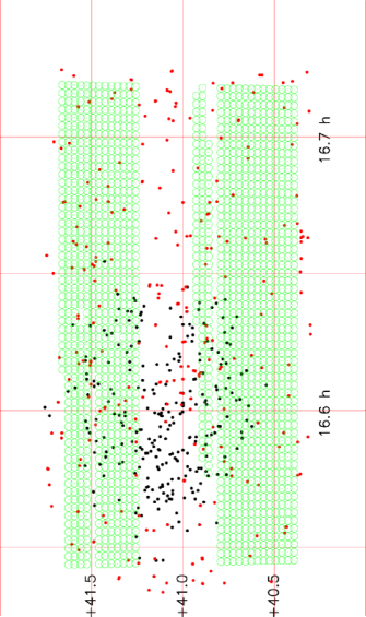
Figure 1: The observing grid (Dec vs. RA, J2000) for our 1627 independent snapshot observations with the VLA at 43 GHz. The green circles represent the approximate size of the synthesized fields; the field-centre separation is twice the FWHM of the primary beam. Red dots mark source positions from the FIRST catalogue (Becker et al. 1995); black dots show source positions from the ELAIS N2 1.4-GHz catalogue (Ciliegi et al. 1999).

Surveying at frequencies as high as 43 GHz is not straightforward, as this pilot study will demonstrate. Hence this paper does not follow the conventional survey, analysis, catalogue, source-count etc. route – the data do not lend themselves to such a procedure. We thus present a road map for orientation.

1. § 2 Survey Design considers why we chose the region ELAIS N2 and how we came to the plan for coverage in terms of independent snapshots of given cycle parameters. The Appendix A1 describes an analysis leading to this design.

2. Observations and Reductions (§ 3) constitutes the conventional part of the paper. We used standard AIPS analysis routines.

3. The 1627 independent snapshot images show many source-like deflections, as decribed in § 3. With our lack of knowledge of the sky at 43 GHz, we try in § 4, Finding Real Sources to use as many avenues as possible to explore the reality of these deflections. To do so, we select a sample of deflections from all snapshot images down to a level of 3 times the rms noise level on each image. It is essential to emphasize at the outset that we never use a 3$\sigma$ sample in a source-counting process, as the effects of Eddington bias are lethal at such levels. However the sample gives us the broadest scope to establish the frequency of real detections, and we try to do this by examining the statistics of the sample, the coincidences of deflections with known sources from radio catalogues at other frequencies, and the coincidences with optical counterparts using the Palomar II Sky Survey and the Sloan Digital Sky Survey.

4. The minimal returns from the exercises of § 4 led us to consider how to use the survey data to estimate the source count at 43 GHz. We do so in § 5 by analyzing the imprint of the primary beam shape on the expected radial distribution of sources in the collective images, and we develop a technique for this that uses each deflection, real or otherwise, in a maximum-likelihood analysis.

5. Finally (§ 6) we compare the results of this analysis with estimates of counts at other mm-wavelength frequencies.

2 Survey design

We chose the ELAIS N2 region as having a wealth of information available from surveys at radio to X-ray wavelengths (see e.g. Rowan-Robinson et al. 2004). Moreover a bright calibrator (3C 345, 1642+398) stands close by, essential for observations at this frequency.

To find the maximum number of sources, given source counts of slopes with which we are familiar in the radio regime, the worst survey strategy is a single deep exposure, which we estimate would have yielded $\leq$ 0.05 sources in the primary beam (1.00 arcmin Full-Width Half-Maximum = FWHM) area, assuming a 24-h integration and an rms of 250 $\mu$Jy in 10 min. At radio wavelengths, wide and shallow always beats narrow and deep; an analysis in Appendix A1 quantifies this and shows that our adoption of the NVSS observing cycle (23 sec integration, 7 sec telescope settle) is near optimal for a series of independent snapshots. We estimated from the Ryle Telescope 15-GHz source count available at the time that observing 2880 fields in 24h should yield about 5 sources at a 4 mJy ($\sim 4\sigma$) survey limit. There is no significant difficulty in analysis of such a number of fields; this is essentially a mapping process and the general emptiness of the sky at 43 GHz implies that almost no deconvolution is required.

We used the technique of ‘referenced pointing’ (see www.vla.nrao.edu/memos/test/189/) to position the primary beam with an accuracy of better than 5 arcsec.

3 Observations and Reductions

The observations were made in late 2001, at which time all VLA antennas had been newly equipped with 43-GHz receiving systems. In order to maximize sensitivity to extended emission and to minimize the effects of the atmosphere on phase stability, we used the the smallest VLA, i.e. the D configuration; and we observed in November, as the necessary phase stability at this frequency is generally available only in winter. We observed in 4 6-hour runs to keep to higher elevations, so as to minimize atmospheric effects.

During the 24 hours of observing allocated to the programme, we made 1627 independent snapshot observations, on the grid shown in Fig. 1. Field centres are separated by 120 arcsec, twice the primary-beam FWHM. The observations were carried out 02, 03, 12 and 23 Nov, 2001, in outstanding weather conditions for the first three sessions, clear or less than 20 per cent cloud. The final 8-hour session was disrupted by rain, snow and cloud, with wind forcing the array to be stowed for much of this period. This resulted in the gap at the central declinations of Fig. 1. About 19.0 useable hours of observations were obtained as judged from the phase stability, and out of 24h this is good fortune at frequencies as high as 43 GHz.

The primary beam FWHM is 1.00 arcmin and the synthesized beam FWHM 2.3 arcsec. The phase calibrator 3C345 (1642+398) was observed approximately every 30 minutes. For flux density calibration, once or twice per session we observed 3C 286 (1331+305), with a flux density of 1.45 Jy at 43.4 GHz. The effects of slight resolution at this frequency were removed via the appropriate VLA model supplied in the NRAO AIPS software package.

We used standard AIPS procedures in the analysis. At each field centre we made a map of $1024\times 1024$ pixels each 0.2 arcsec square, total map extent $3.4\times 3.4$ arcmin. We used a minimal CLEAN (100 cycles, gain=0.1, $\leq$80 components $\geq$1 mJy) on each map; this procedure unfortunately proved necessary in order to use subsequent AIPS routines, which require CLEANed data as input.

In order to examine whether our phase calibration every  30 minutes was adequate, and in particular to look at potential decorrelation, we carried out a simple experiment on the phase calibration data of the observing day 12 Nov 2001. The phase calibrator was observed for one minute at UT times of 17:11, 17:28, 17:47, 18:04, 18:27 and 18:43. Using AIPS and doctoring the input files, we made three measures of the calibrator flux density, assuming it was a programme source and using phase calibrators either side of it for flux calibration. We thus made a measure of the flux of 1642+398 at 17:28 using the 17:11 and 17:47 observations alone as flux calibrators, and so on for meaures of 1642+398 at time of 18:04 and 18:27. The three values of flux density obtained differed from the input value (9.11 Jy at 43.4 GHz) by +1.5%, +0.1% and +2.7%. We concluded that calibration was satisfactory; these differences are insignificant in comparison with the noise and resolution effects measured for the source-like deflections encountered in the survey.

The final 1627 maps have a median rms of 1.4 mJy, close to that estimated for the survey. The lowest noise maps have an rms of 0.9 mJy; 67 per cent have rms noise $\leq 1.5$ mJy and 98 per cent $\leq 2.0$ mJy. Inspection of the maps shows a number of low-level striations well under the rms noise level, and responses, many of which look source-like. The responses happen because the receiver or sky noise is only introduced at points with measurements in the $uv$ plane. For snapshot observations in particular, this means that with noise partially correlated between antennas the images will show apparently coherent structure even in the absence of any real sources. This will be in the form of intersecting ripples of various periods (one per $uv$ point) with amplitude and phase fluctuating between observations. Responses, fictitious sources, are most easily generated where these ripples intersect. If all source-like responses are spurious and due to receiver noise as described, then there is no imprint of the primary beam in the image from each snapshot, a point discussed in detail in § 4.1 and § 5. Most of these responses are very extended to the 2.3-arcsec beam but many look like unresolved sources. We consider this issue in the following section.

In short, the autocorrelation function of the images is not remotely Gaussian, although the rms noise (in good weather conditions) is close to that predicted from telescope and instrumentation parameters.

The total area covered as a function of flux density was calculated by considering each snapshot field separately, the primary beam and the rms flux density, and adding up the areas available to detect flux density for point sources above given signal-to-noise ratio (s/n). The resulting curves of area versus sensitivity are shown in Figure 2.

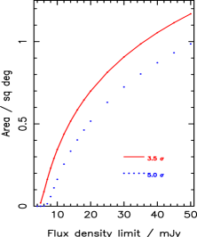
Figure 2: The area surveyed down to a given sensitivity level, where this is taken to be either 3.5 or 5 times the rms noise on each of the 1627 snapshot maps, and the primary beam is taken to be a circular Gaussian with FWHM 60.0 arcsec. It is known that out to a radius of 1 FWHM, this assumption represents the beam well.

4 Finding real sources

We applied the AIPS routine SAD to each map to search for sources, setting a flux limit of 3.0 mJy. We then removed from the subsequent list all objects with peak flux-density to noise ratio below 3.0. This gave us a uniform set of 54225 deflections (an average of 33 per field). Of course a 3$\sigma$ limit is far too low if we were selecting responses for a source list based on s/n alone. Under such circumstances, Eddington bias is extremely damaging and even a 4$\sigma$ limit results in significant contamination of a source list with noise peaks. However, here we are simply selecting a sample to search for possible detections using criteria other than s/n.

The net result of the extensive searches described below is one secure 43-GHz source, the previously catalogued QSO 16382+414 with S${}_{43\,{\rm GHz}}$ = 26 mJy, and several possible 43-GHz sources coinciding with either blue stellar objects or sources previously catalogued at 1.4 GHz.

We reasoned towards establishing real sources detected in the survey via the following steps.

4.1 Source statistics

Fig. 3 shows a diagram for the 54225 ‘sources’ with ratio of integrated to peak emission (‘Size Factor’ or SF) as a function of peak flux density. The diagram demonstrates that attention should be confined to those objects for which this flux ratio is less than 2, and that there may be a set of unresolved detections at $S_{\rm peak}>7$ mJy, $0.5<$ SF $<1.5$ whose reality needs to be examined further.

Responses narrower than the synthesized beam, SF $<$ 0.5, are probably spurious; a number are clearly single-pixel fluctuations. We examined a fair sample of the ‘detections’ both extended and apparently point-like, via visual inspection and profiling of a sample of $3.0\sigma$ detections on the synthesized maps. Most do not look convincing, sitting astride response lines or at the junctions of these lines. There is good reason to confine our attention to the compact ‘objects’. All extended-emission radio sources are known to have synchrotron $\sim$ power-law spectra of spectral index $\alpha<-0.5$, so that sources detected at 43 GHz will almost certainly not show extended emission or be associated with extended radio objects detected at lower frequencies. Moreover many if not most such extended objects would be resolved out by the 2.3-arcsec synthesized beam of the survey. We are looking for compact objects, QSOs or BL Lac objects with flat, inverted and/or variable spectra, probably beamed, and with structures on milliarcsec VLBI scales. However in the interests of objectivity the first of our investigations here retains the entire sample of 54225 responses.

Figure 4 argues strongly against the reality of most of these ‘sources’, even the stronger ones. Here deflection height is plotted against $r^{2}$, the square of the distance from the individual field centres in arcsec. This is effectively area, so that the plot should be uniform if the deflections are random results, e.g. of intersecting response lines. The vertical lines show the value of $r^{2}$ corresponding to the primary-beam half-power point, $r^{2}$ corresponding to twice this, and $r^{2}$ corresponding to half the width of the synthesized square. Deflections corresponding to real sources should be concentrated within $r^{2}_{\rm FWHM}$, and few if any should appear beyond $r^{2}_{\rm 2FWHM}$. The deflections, compact or extended, appear to be depressingly uniform across the full extent of $r^{2}$. We must conclude that the vast majority cannot represent real sources.

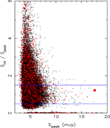
Figure 3: The $3.0\sigma$ ‘detections’ on the 1627 maps, shown in terms of ratio of integrated to peak flux density vs. peak flux density. Red dots are ‘detections’ within a radius of 60 arcsec = 1 FWHM of the field centres; black dots are ‘detections’ at larger distances. Real sources are expected lie within the FWHM distance, and to be unresolved, lying between the horizontal lines at ratios of 0.5 and 1.5. The points along the horizontal axis represent single-pixel responses which are rejected from further consideration by the lower ratio limit. The large red dot represents 16382+414, the known QSO detected in the 43-GHz survey; see § 4.2.

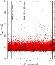
Figure 4: The $3.0\sigma$ ‘detections’ on the 1627 maps, plotted against the square of the distance in arcsec from each field centre. Red dots are detections for which the ratio of integrated to peak flux lies between 0.5 and 1.5, i.e. unresolved to the 2.3-arcsec synthesized beam; black dots are all other deflections. There is no noticeable concentration of the high s/n deflections to the primary beam response denoted by vertical lines corresponding to the FWHM and $2\times$FWHM; the distribution looks uniform with $r^{2}$, indicating that most responses do not represent real sources.

4.2 Coincidences with catalogued sources?

We compared all 54225 ‘source’ positions with those for radio sources in the ELAIS N2 catalogue (Rowan-Robinson et al. 2004) from the 1.4-GHz deep surveys of this region (Ciliegi et al. 1999; Ivison et al. 2002; Biggs & Ivison 2006), and with the sources of the FIRST survey (Becker et al. 1995) There were a total of 538 such sources within our synthesized area (Figure 1). We confined attention to those within 10 arcsec of catalogued sources; the properties of these objects were found not to differ from the others. We then examined carefully all the objects lying within 2 arcsec of the catalogued sources. The total coincidence area corresponding to 2 arcsec radius suggests a possible 5.4 coincidences due to chance. We found a total of 15 such coincidences. We then confined attention to objects with size factors of 1.5 or less; the list of such coincidences totalled six.

(With regard to this SF $<1.5$ upper limit, it could be argued that it should be relaxed to somewhat larger values at lower signal-to-noise. We carried out Monte-Carlo trials, and found that although as expected for point sources there is a distinct increase in observed SF for true point sources as signal-to-noise is lowered to the $3\sigma$ threshold, only some 5 per cent of the trials yielded SF values above 1.5. Thus the above list of 6 possible coincidences above may be short by half-a-source statistically; but on the other hand, relaxing the criterion feeds in a far greater proportion of assuredly spurious ‘detections’.)

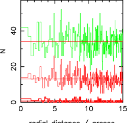
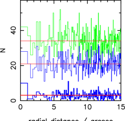
Figure 5: The radial distributions for optical objects from the SSS in equal-area annuli about the field centres for the sample of 16331 source-like deflections. Each annulus has the same area as the central circle of radius 1.06 arcsec. Random association of optical and radio objects should show a flat histogram with Poisson noise superposed. In both left and right panels the upper histogram (green) is for all objects down to the limit of the SSS survey, for source-like deflections within 80 arcsec of the synthesized field centres. Left panel: galaxies, as classified in the SSS object lists, are shown as the middle and lowest distributions, the middle distribution for all galaxies, the lower for blue galaxies with $m_{b}-m_{r1}\leq 1.0$. Right panel: the central histogram is of all objects classified by SSS as stellar, while the lower histogram is for bluish stellar objects with $m_{b}-m_{r1}\leq 1.40$ and $m_{r1}\leq 20.2$).

Of these 6 coincidences within 2 arcsec, we rejected two as possibilities because the FIRST 1.4-GHz contour maps suggest that the catalogued source is a component of a double-structure radio source. An inverted radio spectrum object has never been seen as a lobe of a double radio source and it is thus highly unlikely that the 43-GHz deflection is real. Of the remaining four sources, three lie more than 60 arcsec from their field centres, and none has a candidate optical identification down to the limits of the SDSS (Sloan Digital Sky Survey). The probability of finding real sources beyond one FWHM from the beam centre is minimal, and in each case, supposing the source is real, the beam correction would result in flux densities at 43 GHz of from 120 mJy to $>$1 Jy. Such extreme spectrum objects would have been detected should they exist; and the lack of any optical counterpart above SDSS limits results in a further drastic reduction in probablity that these objects are anything other than artifacts. The closest of these to the field centre, 16392+408, lies 62 arcsec off axis, and correction for the primary beam attenuation would give it a flux density at 43.4 GHz of $\sim$120 mJy. The coincident FIRST source has a flux density of 22.1 mJy at 1.4 GHz. It is entered in Table 1 as a candidate source, albeit an improbable one.

Of the 6, this leaves one final coincidence to consider, and here there is no doubt of the reality of the source at 43.4 GHz; it has a s/n of 9.6. The object is 16382+414, a flat-spectrum QSO known to have a redshift of 2.2, apparently variable as the Ciliegi et al. (1999) and FIRST flux densities (24.3 and 37.3 mJy respectively at 1.4 GHz) differ significantly. The details of this object are in Table 1 (bold typeface). This real source is the strongest compact response within $0.5\times$ FWHM = 30 arcsec of the individual field centres. It may be slightly extended to the 2.3-arcsec sysnthesized beam.

The yield (of $\sim$one coincidence) is small but instructive. The secure coincidence with 16382+414 guarantees that the survey and reduction procedure is capable of finding real sources. It also ensures that the coordinate systems are in coicidence to better than 1 arcsec, so that other coincidences, either with previously catalogued radio sources or with optical identifications, are possible. It does not rule out the possibility that some ‘sources’ close to the $3.0\sigma$ limit in s/n are real, but the coincidence results plus Figures 3 and 4 indicate that the great majority are not.

4.3 Optical identifications?

The AT20G survey (Ricci et al. 2004; Sadler et al. 2006; Massardi et al. 2008) suggests that compact objects over the range of flux densities sampled by the survey (20 - 500 mJy at 20 GHz) are identified predominantly (50 to 80 percent) with blue stellar objects, QSOs or BL Lacs. A small proportion is identified with relatively bright galaxies. A further way then of searching for real sources amongst the 54225 deflections is to look for optical coincidences, primarily stellar counterparts. It is possible to do this in bulk because of the ease with which automated comparisons can be done with both POSSII and UKSTU sky surveys, thanks to the SuperCosmos Sky Survey (SSS).

To carry this out, we reduced the sample of 54225 as follows. We first placed a stringent SF criterion to confine ourselves to compact ‘detections’, using only those ‘sources’with $0.6<{\rm SF}<1.4$. This reduced the sample to 26090. (Again it could be argued that we are throwing away possible real sources because of the increasing spread in SF at lower signal-to-noise; again we argue that we are after a set of unambiguous detections, which if present would lead us to carry out a more rigorous source cataloguing process. We found no encouragement to do this.) We then threw away responses in the field ‘corners’ by setting a generous radius limit of 80 arcsec, (c.f. half-power beamwidth of 60 arcsec); deflections further off centre than this require (poorly known) beam-factor corrections so large as to make them Jy-level sources. The sample is now 16331 in size. We examined all 16331 position on SSS R-band images, easy to automated with the provision of object catalogues in the SSS download which list magnitudes, positions, and object type (galaxy/stellar discrimination) for all objects above the detection limit in each postage-stamp image.

Figure 5 shows a histogram of surface densities of the optical objects in equal-area annuli, 200 annuli out to a distance of 15 arcsec from each deflection position. The beam is small enough (FWHM 2.3 arcsec) so that true identifications should lie in the first area, the central circle of radius 1.06 arcsec. The surface distribution of all optical object types (upper histograms) shows a positive signal in this bin of little significance. If the distribution of objects classed in SSS as galaxies is considered (left panel) there is nothing of note – apparently no coincidences (although statistically a few identifications, say $\leq 5$ cannot be ruled out). The right panel tells a different story for stellar objects, which we might expect to be QSO or BL Lac identifications – the distribution for all ‘stars’ shows an excess in the central bin at a level of $2.8\sigma$. We examined the distribution of SSS $m_{b}-m_{r1}$ colours vs $m_{b}$ for the sample of FSRQ of Jackson et al. (2002) and this shows that FSRQ are confined to a region of the colour – magnitude plane with $(m_{b}-m_{r1})<1.4$, $m_{r1}>20.2$. (We used the SSS magnitude system, in which our $m_{b}=B_{j}$, and our $r_{1}=ESO-R/POSS-IE$.) Applying this cut to the stellar objects (and in addition requiring that the objects lie within 60 arcsec of the field centre) yields the lower distribution in Figure 5, right panel. The excess in the central circle now runs at $4\sigma$; there are 10 objects and the mean value is 3. The implication is that a few ($\leq 7$) of the the blue stellar objects may be real identifications and that this number of deflections out of the 16331 may be real sources. The QSO 16382+414 is amongst these coincidences, rediscovered yet again by this automated identification technique, and as well, one of the 10 objects proved to be a galaxy when examined with the higher resolution of the SDSS.

Using SDSS photometric data, we plotted the remaining 8 stellar objects in the central annulus (10, minus the QSO 16382+414, minus the galaxy) in Figure 6 as the large black filled circles. The known QSO is plotted as the large blue filled circle. In the same plot we also placed the photometric colour data (black dots) for the 27 of the 28 objects falling within the inner circle of 1.06 arcsec radius (central distribution in right panel of Figure 5), again omitting the galaxy; the 9 objects (8 stellar, one QSO) already plotted are of course a subset of these 28 objects. These objects, particularly the brighter ones, generally follow the black-body locus for hot stars. As a control sample we plotted the SDSS $(u-g)$ vs. $(g-i)$ colours for a sub-sample of FSRQ from the Jackson et al. (2002) catalogue, namely those from the full sample which fell within the SDSS area, a total of 26. These generally cluster at values of $(u-g)$ below the stellar sequence, and the known QSO in the sample of 27 stellar objects falls in with these other FSRQ. The few FSRQ of the Jackson et al. (2002) sample with redshifts greater than 2.5 (crosses) streak away to high values of $u-g$ as is well known (see Weinstein et al. 2004); the absorption shortward of Lyman-$\alpha$ gives relatively larger values of $u$). There is a small region near $(u-g)=1.0$, $(g-i)=0.4$ which appears common to the stellar sequence and to FSRQ with $z\sim 2.5$. Some 6 of the stellar objects coincident with 43-GHz deflections lie close to this region, and might be considered as possible identifications; this number would certainly account for the bulk of the statistical excess. Three of these are in the original sample of 8 likely candidates, while of the other three, two have distances from the filed centres of just over 60 arcsec and the third is fainter than the $m_{r1}=20.2$ limit.

There are, however, indications that most of these objects are not identifications and the deflections are consequently not real sources.

1. Stacking the FIRST FITS images of these 6 objects, or the 8 objects of the most probable identifications, or indeed the 26 stellar objects within the 1.06 arcsec radius, yields total absence of any central response. Mean flux densities at 1.4 GHz must lie below levels of $\sim 0.1$ mJy, leading to putative spectral indices of $\alpha_{1.4}^{43}>1.5$.

2. If the deflections were real sources, then they should cluster within the FWHM of the primary beam, i.e. within 30 arcsec of their field centres, and certainly within a radius of 2FWHM (as in Figure 7, left panel). In fact the radial distribution of the 26 objects relative to their field centres is as follows: within 20 arcsec – 2, between 20 and 40 arcsec – 4, between 40 and 60 arcsec – 10; between 60 and 80 arcsec – 10. The corresponding numbers for random distribution, i.e. according to annular area, are 2, 5, 8 and 11. The distribution thus appears random; there is no indication that these ‘sources’ were selected by beam response. This is equally true for the sub-sample of 8 likely identifications, and the sub-sample of 6 objects with colours close to the FSRQ locus.

3. Finally, all the redshifts would need to be clustered in a small range of z, i.e. $2.5\pm 0.2$. This is unlikely; the range is not at the peak or centroid of the redshift distribution for FSRQ (Jackson et al. 2002).

   Despite the low probability that these 6 ‘sources’ are real, they have been listed in Table 1.

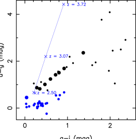
Figure 6: Colour – colour diagram using SDSS photometry for 27 of the 28 objects which are stellar and within 1.06 arcsec of deflection positions. (SDSS shows one of the 28 ‘stellar’ objects from the UKST SSS to be a galaxy.) Of these objects 26/27 are shown as black filled circles; the 8 larger of these are the objects selected from the SSS catalogues as having $m_{b}-m_{r1}\leq 1.4$ and $m_{r1}>20.2$. The known QSO identification in the set of 27 stellar objects (16382+414) is shown as the large blue filled circle. Smaller blue filled circles represent the SDSS photometric data for 26 FSRQ from the sample of Jackson et al. (2002) which lie in the area covered by SDSS. These cluster at values of $u-g$ significantly below the star relation, with four exceptions: the four higher-redshift ($z>2.5$) QSOs marked as crosses shoot to high values of $u-g$ because of the increasingly large $u$ magnitudes due to absorption below the Lyman-$\alpha$ line (Weinstein et al. 2004).

We have to conclude that the majority and possibly all of these candidate identifications (exept for the known QSO) are chance coincidences, with the high response in the central bin of Figure 5 (right panel) a statistical anomaly. It could still be that in addition to the known QSO, one to three of 6 sources listed as stellar in Table 1 may be real. Direct observations, either confirmatory radio observations or optical spectra of the putative counterparts, are needed in this respect. Finding charts are readily available using the SDSS navigate tool http://cas.sdss.org/astrodr7/en/tools/chart/navi.asp.

Table 1: Source list: coincidences with stellar counterparts and catalogued sources

Source	RA	Dec	dist1	$S_{p}(43)^{2}$	$S_{\rm corr}$(43)3	$S$(1.4)4	$\alpha^{5}$	$g^{6}$	$u-g^{6}$	$g-i^{6}$	type7
16338+404	16:33:49.92	40:25:21.9	51.5	4.2$\pm$1.4	32.5	$<$0.1	$>$0.9	18.17	1.01	0.47	stellar
16345+406	16:34:32.18	40:41:47.6	59.5	4.2$\pm$1.3	64.2	$<$0.1	$>$1.5	17.61	0.87	0.28	stellar
16345+415	16:34:34.06	41:30:55.8	39.3	4.3$\pm$1.4	14.0	$<$0.1	$>$1.2	18.77	0.82	0.35	stellar
16349+405	16:34:58.73	40:32:34.3	59.7	5.1$\pm$1.7	79.4	$<$0.1	$>$1.9	21.75	1.11	0.38	stellar
16361+405	16:36:06.44	40:31:24.0	53.2	4.8$\pm$1.6	42.4	$<$0.1	$>$1.8	22.04	0.76	0.53	stellar
16377+416	16:37:47.27	41:38:32.4	61.3	4.2$\pm$1.4	75.9	$<$0.1	$>$1.9	19.57	1.05	0.21	stellar
16382+414	16:38:17.32	41:27:29.5	22.4	17.6$\pm$1.8	25.9	37.3	-0.11	19.93	0.45	0.06	QSO, z=2.2
16392+408	16:39:12.05	40:52:35.8	61.9	6.2$\pm$1.8	118.5	22.1	+0.49	-	-	-	FIRST coinc

1Arcsec distance of deflection from primary-beam axis.

2mJy peak deflection flux density at 43.4 GHz.

3mJy 43.4-GHz flux density corrected for primary beam attenuation.

4mJy 1.4-GHz flux density from FIRST survey: catalogue or stacked images.

5Spectral index 1.4 - 43.4 GHz, $S\propto\nu^{\alpha}$.

6Magnitudes, from SDSS photometry.

7stellar – coincidence with blue stellar object to within 1.06 arcsec; QSO – catalogued quasar; FIRST coinc – coincidence with

catalogue source, FIRST survey.

5 A statistical estimate of the 43-GHz source count

There is a way to use the deflection statistics alone (randoms and reals) to estimate the source count. This is based on the primary beam response, which should leave a significant imprint on source distribution if even a small proportion of the sources are real, so small a proportion as not to be detectable in individual fields. The effect is dependent on source-count slope, enhanced when the source count is steep.

Consider an integral count of power-law form (and over the short flux range sampled, this is a perfectly adequate description), $N(>S)=KS^{-\gamma}$, and a round beam of Gaussian shape

$$f(r)={\rm exp}[-4{\rm ln}2r^{2}/\Delta^{2}],$$ (1)

where $\Delta$ is the FWHM of this Gaussian (i.e. the variance for the Gaussian is $\sigma^{2}=\Delta^{2}/8{\rm ln}2$). If we can detect a source of $S_{0}$ Jy at the centre of the beam, then the source density here is $N(r=0)=KS_{0}^{-\gamma}$; but if it is away from the centre, the source density must fall off as

$$N(r)=K(S_{0}/{\rm exp}[-4{\rm ln}2r^{2}/\Delta^{2}])^{-\gamma}$$ (2)

If $\gamma=1$ then the source detection level is $\propto$ (1/beam factor); but if $\gamma$ exceeds $1$, taking say the Euclidean value of $1.5$, then the falloff in source density is more rapid than the beam shape implies. Fig. 7 shows how this can be used to estimate $K$. Note that no values of flux density need to be measured (except to set the survey limits). The result depends on a radial counting of source numbers alone. This is an illustrative approach; we now describe a greatly improved likelihood technique.

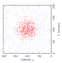
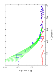
Figure 7: A simulation to show how primary beam response can be used not only to distinguish the proportion of true detections, but also to measure source count parameters. The simulated field (to the scale of the current maps) is shown at the left. It has 1000 randomly placed ‘deflections’ or unreal responses (blue dots), and the primary beam is aimed at a radio population with a power-law source count of $N=KS^{-\gamma}$, where $\gamma=1.5$. We supplied 10000 sources above 1 Jy in the total field of 204.8² arcsec². We set the detection limit at the centre as 1.0 Jy; the beam adopted is Gaussian with FWHM = 60 arcsec. Selecting randomly from the source count gives the set of red dots, falling off rapidly away from the centre as equation 2 indicates. The right diagram shows the resulting radial distribution in histogram form (blue; the histogram of random background deflections alone is red). The radii were chosen so that equal areas are encompassed by all annuli, i.e. $r_{j}=\sqrt{(}C/\pi+r_{j-1}^{2})$. The models shown (green curves), calculated from equation 2 with the 1000 uniformaly-random deflections added, have $K$ running from 0.18 (lower) to 0.28 (upper); there is a clear selection at $K=0.23\pm 0.02$ from the minimum chi-squared test. The value of $K$ we anticipate is $10000/204.8^{2}=0.238$ sources per unit area at a flux density of 1 Jy.

To set this up as a Maximum Likelihood problem, suppose first that there are no fake sources, no noise-simulated source-like deflections, and the distribution of flux densities is given by an integral source count law of the form $N(>S)=KS^{-\gamma}$. We choose annuli, radial elements, small enough that their occupancy is either no deflection+sources, or one at maximum. The $\cal L$(ikelihood) function for the $i^{\rm th}$ object is the probability of observing one object in its $r_{i}$ element times the probability of observing zero objects in all other $r_{j}$ elements accessible to it. The Poisson model is the obvious one for the likelihood:

$$f(x:\mu)=\frac{{\rm e}^{-\mu}\mu^{x}}{x!},$$ (3)

where $\mu$ is the expected number. If $x=1$, the function is $\mu{\rm e}^{-\mu}$ and if $x=0$ it is ${\rm e}^{-\mu}$.

The expected number $\mu$ as a function of radial distance $r$ igiven by

$$\mu=\lambda(r)2\pi rdr,\ \ \mbox{with}\ \ \lambda=KS^{-\gamma}dS,$$ (4)

and

$$S=f(r),\ \mbox{where}\ f(r)=(S_{0}/exp[-4{\rm ln}2r^{2}/\Delta^{2}])^{-\gamma}.$$ (5)

To avoid arithmetic, we divide the area radially into one central circle and $N-1$ annuli about this, each of area $2\pi rdr=a_{i}$, and we design all the radius elements and the central circle to have the same area $a_{i}=a$ (see caption to Fig. 7). We get $\mu(r)=Kf(r)a$, so that for a total of $n$ sources ($N>n$),

$${\cal L}=\prod_{i}^{N}\lambda(r_{i})a\,{\rm e}^{-\lambda(r_{i})a}\,\prod_{j\neq i}^{N}{\rm e}^{-\lambda(r_{j})a}\!,$$ (6)

where $i$ denotes the element of the $r$ plane in which sources are present and $j$ denotes all others. From this, if $s=-2\,\ln\cal{L}$, then

$$s=-2\sum_{i=1}^{n}\,\ln f(r)_{i}-2N\mbox{ln}(Ka)+2Ka\sum_{i}^{N}f(r)_{i}.$$ (7)

As a check at this point, if we set the derivative of $s$ with respect to $K$ to zero, we get a maximum-likelihood estimate for $K$:

$$K_{0}=\frac{n}{a\sum_{i}^{N}f(r)}=\frac{n}{a\sum_{i}^{N}[S_{0}/exp(-4{\rm ln}2r^{2}/\Delta^{2}]^{-\gamma}}.$$ (8)

Moreovoer if $\Delta=\infty$, i.e. an infinitely broad beam, and we set $Na=A$, the total area surveyed, this reduces to $N=K_{0}\,S_{0}^{-\gamma}\,A$, i.e. the number of sources observed is the source-count per unit area times the area surveyed.

We now add a random uniform background of fake ‘sources’, at a density of $C$ sources per unit area. (Note that there is no assumption of an intensity distribution for these; this likelihood technique depends solely on surface density.) We get the value of $\lambda=KS^{-\gamma}dS+C$, so that $\mu=a(KS^{-\gamma}dS+C)$. With the same analysis as above, we find

$$s = -2\sum_{i}^{n}{\rm ln}(Kf(r)_{i}+C)-2(n{\rm ln}(a)+aCN)$$ (9)

$$+2Ka\sum_{i}^{N}f(r)_{i}.$$

There is now no simple differentiation to find a best estimate for $K_{0}$. Of course, setting $C=0$ recovers the results of equations 7 and 8.

The only point we now need to address is how to do this for 1627 fields combined, the problem being that each field has a different value of $S_{0}$, the detection limit, because each field has a different value of rms noise. The path towards this is straightforward, as shown in Fig. 8. This simulation models the real-life situation by taking five simulations each using the same source count and beam parameters, and choosing five different values for detection levels $S_{0}$, at 1.0, 2.0, 3.0, 4.0 and 5.0 Jy. Of course higher values of $S_{0}$ yield far fewer detections of sources. With the same number of randoms in each field, the likelihood function thus broadens rapidly with increasing $S_{0}$. Likelihoods are multiplicative, so that only addition (and normalization) of the likelihood functions computed for all fields is required. The anticipated value of $K$ is retrieved as shown.

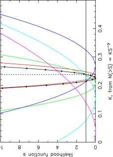
Figure 8: This simulation adopts the original simulation parameters, but now selects 5 fields with the same initial source count. The random uniform-background samples added to all five fields have the same surface density, but the five have different cutoff-sensitivity ($S_{0}$) values of 1.0, 2.0, 3.0, 4.0 and 5.0 Jy. Randomly-selecting from the original source count via the 60-arcsec beam results in samples of 595, 212, 111, 80 and 66 sources respectively, the number decreasing as the survey sensitivity is decreased. The results of the likelihood calculation are shown by the curves of likelihood function $s$, red for 1.0 Jy, green for 2.0, blue for 3.0, turquoise for 4.0 and magenta for 5.0. The function broadens rapidly as we lose sources with reduced sensitivity – see text. The black curve is the sum; the black line at $\Delta s=1.0$ indicates the approximate $\pm 1\sigma$ value so that the $\pm 1.0\sigma$ range of K for each of the 5 realizations (and for the summed black curve) is given by the range of $K$ between the intersections with this line. The derived value of $K$ from the summed (black) curve is is $0.23$ cf the true value of 0.238.

To perform the experiment on the results from the survey, we again reduced the total number of sources by limiting the total list of $>3.0\sigma$ detections to those which could be point-like. We adopted the slightly more stringent limits of $0.6<{\rm SF}<1.4$, yielding a total of 26090 ‘sources’. Plotting these in a histogram analogous to Figure 7 showed no indication of an increased surface density at the smaller radii, a clear indication that the likelihood calculation will yield only an upper limit to $K$. Because individual fields have very small numbers of objects (mean = 26090/1627 or $\sim 16$) on which to perform the likelihood calculations, we ordered the fields according to their rms values and added them together in 74 batches of 22. We then used the mean value of the rms=$\sigma$ for each batch of 22 to calculate a single value of $S_{0}=3.5\sigma$ for each group of 22 fields. We adopted a 60 arcsec beam and a value of $\gamma=1.15$ from the estimate of Waldram et al. (2007). We calculated the likelihood function for each of the 74 batches for a range of values of $K$, and summed the results. The final curve of $s$ vs $K$ is shown in Figure 9.

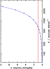
Figure 9: The run of likelihood function $s$ vs $K$, the source-count normalization, summed for the 74 batches of 22 fields each at the points shown. There is no minimum; the imprint of the beam in the data is too weak to be detected, so that the likelihood function provides only an upper limit to the source-count normalization $K$. The intersection of horizontal line at $s=1$ indicates the value of $K~{}(=652.5$) corresponding to a 1$\sigma$ (68 per cent) upper limit.

When converted to probabilities, this curve allows the construction of an integral source count probability region at 43 GHz (Figure 10) in the following way. Because the likelihood function curve (Fig. 9) has no minimum, i.e. the imprint of the beam function is not seen against the background of (almost completely) spurious ‘sources’, the likelihood calculation only provides an upper limit to $K$. Translating the likelhood function into probabilities yields the upper-bound probability contours in Fig. 10. As for the lower-limit probability contours, we know that the survey found a minimum of one source (16382+414). Knowing the total area covered (Figure 2), from Poisson statistics we can compute a lower-limit set of probability contours for surface density. The range over which our estimate of the source count pertains can be set at the high flux-density end with recourse to the source count estimate itself, taking 100 per cent as the probability of finding one source at the flux density of 16382+414 and adopting the (integral) slope value of -1.15. At the low-intensity end, we formed the distribution of values of $\sigma$ for all 1627 fields and assumed a detection threshold of $3.5\sigma$ to calculate a histogram of detection-level probability.

Also shown in Fig. 10 is the 43-GHz count estimate of Waldram et al. (2007), the counts from the WMAP 43-GHz source list (Wright et al. 2009), and the parametric forms of counts at 20 GHz and 95 GHz, as presented by Sadler et al. (2008). We also include the results from Mason et al. (2009) at 31 GHz, an integral source count estimate in the range 1 to 4 mJy of $N(>S)=(16.7\pm 1.7)(S/1\,{\rm{mJy}})^{-0.80\pm 0.07}$ deg^-2. It must be emphasized that of the data in this diagram, only our 43-GHz point and contours plus the WMAP source count represent direct observations at 43 GHz. The other direct observational result in the diagram is the representation of the 20-GHz souce count from the AT20G survey. All other data are inferred or projected from 31 GHz, 43 GHz or 95 GHz. There is no scaling of any result in the diagram.

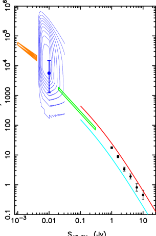
Figure 10: An integral source count at 43 GHz. The blue contours outline a region of probability derived from the VLA 43 GHz survey as described in the text; they are at $p=0.1,0.2\ldots 0.9$. The single blue point at 10 mJy is from the one certain source detected in the survey. The black points at the high flux densities are from the WMAP all-sky survey (Wright et al. 2009). The green region describes the prediction at 43 GHz by Waldram et al. (2007) based on spectra and the 9C survey at 15 GHz. The red curve is the parametric representation of the AT20G counts at 20 GHz, and the turquoise curve shows the parametric form of the count estimated at 95 GHz (Sadler et al. 2008). The orange region describes the 31-GHz count estimate by Mason et al. (2009) from GBT measurements at this frequency of a sample of sources from the NVSS 1.4-GHz catalogue. No scaling has been applied to these or the 20-GHz and 95-GHz results from Sadler et al. (2008). The only direct measurements at 43 GHz are from the present set (blue contours and point) and the WMAP all-sky survey (black points).

6 Discussion and Conclusions

1. This 43-GHz survey (VLA D-array) reaches approximately 7 mJy over an area of 0.5 deg², with a primary beam of 1.0 arcmin FWHM and a circular synthesized beam of 2.3 arcsec FWHM. Done in snapshot mode to follow the ‘wide-shallow’ dictum, it found many apparent sources, most of which on inspection proved to be at the junction of response lines. Most can be eliminated on this basis, and on the basis that they are extended to the 2.3 arcsec synthesized beam. The radial distribution likewise makes it evident that the overwhelming majority of the deflections are not real sources.

2. However the survey does detect real sources, the flat-spectrum QSO 16382+414 for certain, and some additional not-very-probable candidates (Table 1) for which further observations are required. One of these is coincident in position with previously-catalogued sources at 1.4 GHz; there is no candidate identification above the limits of the SDSS. Of the 6 other ‘sources’ in the table, all are coincident with blue stellar objects close to the region occupied by $z\sim 2.5$ FSRQ. These putative 6 sources all must have extreme inverted spectra because stacking suggests that the average flux density at 1.4 GHz must be below 0.1 mJy.

3. We have developed a likelihood method to estimate source counts in a synthesis survey which has thrown up a combination of real and random sources. The method examines the radial distribution in each synthesized field, and because the real sources should decrease with radial distance from the field centre in a predictable manner, in principle both the source-count normalization and the source count power-law index can be determined. With this process, neither detailed cataloguing of the sources nor a priori decisions about which deflections are real are necessary. We have applied this method to the present data, but the dominance of random deflections (by a ratio of perhaps 10000:1) is such that only an upper limit to the surface density of real sources can be derived. No information on the slope of the count is available from the present data; we have adopted a slope estimate for the appropriate flux-density range from Waldram et al. (2007), although the resulting upper-limit contours are relatively insensitive to this.

4. The present results are consistent with extrapolating the count estimate of Waldram et al. (2007), and with the 31-GHz count estimate of Mason et al. (2009), but suggestive of a somewhat higher source surface density than found in either investigation. Such a surface density enhancement might account for the excess signal at $\ell>2000$ found by CBI. We note that the De Zotti et al. (2005) count models, calculated at high frequencies from detailed synthesis of populations from lower-frequency surveys, lie significantly above the count estimates of Waldram et al. (2007).

5. In terms of individual sources, the 43-GHz survey yield is small and provides no direct evidence that any new types of inverted-spectrum sources appear at mJy levels. The lower bound of our error box in Fig. 10 is strongly dependent on the certain detection of a single source; if any of our candidate sources of Table 1 should prove to be real, then a count enhanced above the Waldram et al. (2007) estimate becomes probable. Any such sources will have extremely inverted spectra, as we and Mason et al. (2009) have noted.

6. The observations indicate that there are considerable challenges involved in a snapshot synthesis survey at a frequency as high as 43 GHz.

Acknowledgements We thank Chris Willott for helpful discussions about field choice. We are very grateful to Barry Clark for his efforts in scheduling the VLA to accommodate a late improvement in our observing proposal. Jim Condon proferred useful advice. Eric Greisen gave much help and advice with running AIPS and checking systems remotely. Melanie Gendre helped with running some of the AIPS procedures. Ron Ekers offered many constructive comments on an early draft. Chris Blake gave useful advice on SDSS data. We thank the referee for helpful comments. JVW would particularly like to thank Katherine Blundell for help with computational issues and and with running AIPS over the past several years. JVW acknowledges support during the course of this work through Canada NSERC Discovery Grants.

The National Radio Astronomy Observatory is a facility of the National Science Foundation operated under cooperative agreement by Associated Universities, Inc.

This research has made use of data obtained from the SuperCOSMOS Sky Surveys (SSS), prepared and hosted by the Wide Field Astronomy Unit, Institute for Astronomy, University of Edinburgh, which is funded by the UK Science and Technology Facilities Council. The SSS Web Site is www-wfau.roe.ac.uk/sss/.

The research also made use of data from the SDSS survey. Funding for the SDSS and SDSS-II has been provided by the Alfred P. Sloan Foundation, the Participating Institutions, the National Science Foundation, the U.S. Department of Energy, the National Aeronautics and Space Administration, the Japanese Monbukagakusho, the Max Planck Society, and the Higher Education Funding Council for England. The SDSS Web Site is www.sdss.org/.

Appendix A Observing strategy

Given an integral source-count of the form $N=KS^{-\gamma}$, integration time $t$ per pointing, and a telescope settle time $t_{s}$, there is an optimum observing strategy to detect the maximum number of sources.

It is easy to show that in the radio regime the maximum number of pointings is optimal; wide and shallow easily beats deep and narrow. In a given time T we can make $T/(t+t_{s})$ pointings. Consider the case for long integrations in which $t_{s}$ is negligible. Then the number of pointings is T/t, and if the equivalent beam area is $A_{o}$ then the area covered is $A=A_{o}T/t$. The flux density limit becomes $S=S_{o}/\sqrt{t}$, where $S_{o}$ is the flux density reached in unit time. The total number of sources found is $N=AKS^{-\gamma}=T/t(S_{o}/\sqrt{t})^{-\gamma}$, or $N\propto Tt^{(\gamma/2-1)}$. Thus until $\gamma>2$, until the source count is steeper than that even at highest radio flux densities, the number of sources is maximized with minimum integration times and maximum number of pointings. In fact at the flux densities in question $\gamma\sim 1$.

Given then that short exposures are required, what is optimum exposure time, in that $t_{s}$ must now come into play? There must be an optimum as if we let $t\rightarrow 0$, $t_{s}$ in itself imposes a maximum number of pointings for zero integration time. So let $t=xt_{s}$. The limiting flux density reached is $S=S_{o}/\sqrt{t}$; the area covered in given observing time $T$ (in which $T/t(1+x)$ pointings are possible) is $A_{o}T/t_{s}(1+x)$. The total number of sources detected will be

$$N(x)=\frac{TAKS_{o}^{-\gamma}}{t_{s}^{1.5\gamma}}\frac{x^{\gamma/2}}{1+x}$$ (10)

maximized at

$$x_{\rm max}=\frac{\gamma}{2-\gamma}$$ (11)

Figure 11: The function of equation 1; the source yield as a function of the ratio $x=t/t_{s}$ where $t$ is integration time per snapshot and $t_{s}$ is the telescope settle time. For an integral source count of the form $N=KS^{-\gamma}$, the dashed curve represents $\gamma=0.9$, the solid curve $\gamma=1.0$ and the dotted curve $\gamma=1.1$.

For $\gamma=1$ the result is particularly simple : $x_{\rm max}=1$, integration time and settle time should be equal. Fig 11 shows the function of equation 1. At $x\geq x_{\rm max}$ the function falls very slowly indeed. This insensitivity to $x$ suggests that a further factor could be considered - how much data do we not need? For $x=3$ we achieve only half the pointings as for $x=1$, and yet the loss of sources is just 15 per cent. The NVSS used a 30s cycle; 23s integration with 7s settle, $x=3.3$, representing a good compromise.

The final factor to consider is whether to overlap the beams to make the survey complete to a limiting flux density or to have them entirely independent in a coarse grid. The argument of the opening paragraph pertains - the answer is to use completely independent beams to yield maximum area at minimum sensitivity. The issue can be quantified, quoting the analysis communicated to us by Jim Condon. The NVSS spacing is overlapped just enough to provide nearly uniform sensitivity to ensure completeness down to a fixed limit (e.g., 2.5 mJy/beam) over areas $>>$ beam solid angle. To maximize the number of detections in a representative sample without achieving completeness, the optimum spacing is anything large enough that successive snapshots have no overlap (i.e. $>2$ FWHM). Then, instead of a survey with uniform sensitivity, the yield is a survey covering a small area with high sensitivity and larger areas with lower sensitivity. The NVSS spacing gives the same sensitivity as the on-axis sensitivity of a single snapshot over an effective area of 1/2 the beam solid angle, or $\pi\theta^{2}/(8{\rm ln}2)$ for a Gaussian beam with FWHM $\theta$ (Condon et al. 1998). A single isolated snapshot has sensitivity directly proportional to the primary power pattern. Since the source counts are roughly power-law with a differential slope of $2.0$ (integral slope of $1.0$), the number of detectable sources in the isolated snapshot will be proportional to the whole beam solid angle $=\pi\theta^{2}/(4{\rm ln}2)$. Thus the yield per unit time with non-overlapping snapshots is twice that with snapshots overlapped as for the NVSS gridding.

Accordingly we adopted the NVSS 30s cycle, 7s settle and 23s integration, and coarse gridding. (A shorter settle time for the VLA would have been an advantage to us.)

References

- [\citeauthoryearBecker, White & HelfandBecker et al.1995] Becker R. H., White R. L., Helfand D. J., 1995, Astrophys. J., 450, 559
- [\citeauthoryearBiggs & IvisonBiggs & Ivison2006] Biggs A. D., Ivison R. J., 2006, Mon. Not. R. astr. Soc., 371, 963
- [\citeauthoryearBolton, Cotter, Pooley, Riley, Waldram, Chandler, Mason, Pearson & ReadheadBolton et al.2004] Bolton R. C., Cotter G., Pooley G. G., Riley J. M., Waldram E. M., Chandler C. J., Mason B. S., Pearson T. J., Readhead A. C. S., 2004, Mon. Not. R. astr. Soc., 354, 485
- [\citeauthoryearBrandie & BridleBrandie & Bridle1974] Brandie G. W., Bridle A. H., 1974, Astron. J., 79, 903
- [\citeauthoryearCiliegi, McMahon, Miley, Gruppioni, Rowan-Robinson, Cesarsky, Danese, Franceschini, Genzel, Lawrence, Lemke, Oliver, Puget & Rocca-VolmerangeCiliegi et al.1999] Ciliegi P., McMahon R. G., Miley G., Gruppioni C., Rowan-Robinson M., Cesarsky C., Danese L., Franceschini A., Genzel R., Lawrence A., Lemke D., Oliver S., Puget J.-L., Rocca-Volmerange B., 1999, Mon. Not. R. astr. Soc., 302, 222
- [\citeauthoryearCondon, Cotton, Greisen, Yin, Perley, Taylor & BroderickCondon et al.1998] Condon J. J., Cotton W. D., Greisen E. W., Yin Q. F., Perley R. A., Taylor G. B., Broderick J. J., 1998, Astron. J., 115, 1693
- [\citeauthoryearDavies, Franzen, Davies, Davis, Feroz, Genova-Santos, Grainge & et al.Davies et al.2009] Davies M. L., Franzen T. M. O., Davies R. D., Davis R. J., Feroz F., Genova-Santos R., Grainge K. J. B., et al. 2009, ArXiv:0907.3707
- [\citeauthoryearDe Zotti, Ricci, Mesa, Silva, d Toffolatti & González-Nuevode Zotti et al.2005] De Zotti G., Ricci R., Mesa D., Silva L., d Toffolatti L., González-Nuevo J., 2005, Astron. Astrophys., 431, 893
- [\citeauthoryearEdge, Pooley, Jones, Grainge & SaundersEdge et al.1998] Edge A. C., Pooley G., Jones M., Grainge K., Saunders R., 1998, in Zensus J. A., Taylor G. B., Wrobel J. M., eds, IAU Colloq. 164: Radio Emission from Galactic and Extragalactic Compact Sources Vol. 144 of Astronomical Society of the Pacific Conference Series, GPS Sources with High Peak Frequencies. p. 187
- [\citeauthoryearFranzen, Davies, Davies, Davis, Feroz, Genova-Santos, Grainge & et al.Franzen et al.2009] Franzen T. M. O., Davies M. L., Davies R. D., Davis R. J., Feroz F., Genova-Santos R., Grainge K. J. B., et al. 2009, ArXiv:0907.3843
- [\citeauthoryearHinshaw, Nolta, Bennett, Bean, Doré, Greason, Halpern & et al.Hinshaw et al.2007] Hinshaw G., Nolta M. R., Bennett C. L., Bean R., Doré O., Greason M. R., Halpern M., et al. 2007, Astophys. J. Suppl., 170, 288
- [\citeauthoryearIvison, Greve, Smail, Dunlop, Roche, Scott, Page, Stevens, Almaini, Blain, Willott, Fox, Gilbank, Serjeant & HughesIvison et al.2002] Ivison R. J., Greve T. R., Smail I., Dunlop J. S., Roche N. D., Scott S. E., Page M. J., Stevens J. A., Almaini O., Blain A. W., Willott C. J., Fox M. J., Gilbank D. G., Serjeant S., Hughes D. H., 2002, Mon. Not. R. astr. Soc., 337, 1
- [\citeauthoryearJackson, Wall, Shaver, Kellermann, Hook & HawkinsJackson et al.2002] Jackson C. A., Wall J. V., Shaver P. A., Kellermann K. I., Hook I. M., Hawkins M. R. S., 2002, Astron. Astrophys., 386, 97
- [\citeauthoryearKellermann & WallKellermann & Wall1987] Kellermann K. I., Wall J. V., 1987, in Hewitt A., Burbidge G., Fang L. Z., eds, Observational Cosmology Vol. 124 of IAU Symposium, Radio source counts and their interpretation. p. 545
- [\citeauthoryearLópez-Caniego, González-Nuevo, Herranz, Massardi, Sanz, De Zotti, Toffolatti & ArgüesoLópez-Caniego et al.2007] López-Caniego M., González-Nuevo J., Herranz D., Massardi M., Sanz J. L., De Zotti G., Toffolatti L., Argüeso F., 2007, Astophys. J. Suppl., 170, 108
- [\citeauthoryearMason, Weintraub, Sievers, Bond, Myers, Pearson, Readhead & ShepherdMason et al.2009] Mason B. S., Weintraub L. C., Sievers J. L., Bond J. R., Myers S. T., Pearson T. J., Readhead A. C. S., Shepherd M. C., 2009, ArXiv:0901.4330
- [\citeauthoryearMassardi, Ekers, Murphy, Ricci, Sadler, Burke, de Zotti, Edwards, Hancock, Jackson, Kesteven, Mahony, Phillips, Staveley-Smith, Subrahmanyan, Walker & WilsonMassardi et al.2008] Massardi M., Ekers R. D., Murphy T., Ricci R., Sadler E. M., Burke S., De Zotti G., Edwards P. G., Hancock P. J., Jackson C. A., Kesteven M. J., Mahony E., Phillips C. J., Staveley-Smith L., Subrahmanyan R., Walker M. A., Wilson W. E., 2008, Mon. Not. R. astr. Soc., 384, 775
- [\citeauthoryearRicci, Prandoni, Gruppioni & SaultRicci et al.2006] Ricci R., Prandoni I., Gruppioni C., Sault R. J., 2006, Astron. Astrophys., 445, 465
- [\citeauthoryearRicci, Sadler, Ekers, Staveley-Smith, Wilson, Kesteven, Subrahmanyan, Walker, Jackson & De ZottiRicci et al.2004] Ricci R., Sadler E. M., Ekers R. D., Staveley-Smith L., Wilson W. E., Kesteven M. J., Subrahmanyan R., Walker M. A., Jackson C. A., De Zotti G., 2004, Mon. Not. R. astr. Soc., 354, 305
- [\citeauthoryearRowan-Robinson, Lari & Perez-FournonRowan-Robinson et al.2004] Rowan-Robinson M., Lari C., Perez-Fournon I., 2004, Mon. Not. R. astr. Soc., 351, 1290
- [\citeauthoryearRowan-Robinson, Lari, Perez-Fournon, Gonzalez-Solares, Franca, Vaccari, Oliver, Gruppioni, Ciliegi & HeraudeauRowan-Robinson et al.2004] Rowan-Robinson M., Lari C., Perez-Fournon I., Gonzalez-Solares E. A., Franca F. L., Vaccari M., Oliver S., Gruppioni C., Ciliegi P., Heraudeau P., 2004, VizieR Online Data Catalog, 735, 11290
- [\citeauthoryearSadler, Ricci, Ekers, Ekers, Hancock, Jackson, Kesteven, Murphy, Phillips, Reinfrank, Staveley-Smith, Subrahmanyan, Walker, Wilson & De ZottiSadler et al.2006] Sadler E. M., Ricci R., Ekers R. D., Ekers J. A., Hancock P. J., Jackson C. A., Kesteven M. J., Murphy T., Phillips C., Reinfrank R. F., Staveley-Smith L., Subrahmanyan R., Walker M. A., Wilson W. E., De Zotti G., 2006, Mon. Not. R. astr. Soc., 371, 898
- [\citeauthoryearSadler, Ricci, Ekers, Sault, Jackson & De ZottiSadler et al.2008] Sadler E. M., Ricci R., Ekers R. D., Sault R. J., Jackson C. A., De Zotti G., 2008, Mon. Not. R. astr. Soc., 385, 1656
- [\citeauthoryearTaylor, Grainge, Jones, Pooley, Saunders & WaldramTaylor et al.2001] Taylor A. C., Grainge K., Jones M. E., Pooley G. G., Saunders R. D. E., Waldram E. M., 2001, Mon. Not. R. astr. Soc., 327, L1
- [\citeauthoryearVieira, Crawford, Switzer, Ade, Aird, Ashby, Benson, Bleem, Brodwin, Carlstrom, Chang, Cho, Crites, de Haan, Dobbs, Everett, George & GladdersVieira et al.2009] Vieira J. D., Crawford T. M., Switzer E. R., Ade P. A. R., Aird K. A., Ashby M. L. N., Benson B. A., Bleem L. E., Brodwin M., Carlstrom J. E., Chang C. L., Cho H., Crites A. T., de Haan T., Dobbs M. A., Everett W., George E. M., Gladders M., 2009, ArXiv 0912.2338
- [\citeauthoryearWaldram, Bolton, Pooley & RileyWaldram et al.2007] Waldram E. M., Bolton R. C., Pooley G. G., Riley J. M., 2007, Mon. Not. R. astr. Soc., 379, 1442
- [\citeauthoryearWaldram, Pooley, Davies, Grainge & ScottWaldram et al.2009] Waldram E. M., Pooley G. G., Davies M. L., Grainge K. J. B., Scott P. F., 2009, ArXiv:0908.0066
- [\citeauthoryearWaldram, Pooley, Grainge, Jones, Saunders, Scott & TaylorWaldram et al.2003] Waldram E. M., Pooley G. G., Grainge K. J. B., Jones M. E., Saunders R. D. E., Scott P. F., Taylor A. C., 2003, Mon. Not. R. astr. Soc., 342, 915
- [\citeauthoryearWallWall2007] Wall J. V., 2007, in G. J. Babu & E. D. Feigelson ed., Statistical Challenges in Modern Astronomy IV Vol. 371 of Astronomical Society of the Pacific Conference Series, Steep Functions in Astronomy: The RQSO z-Cutoff Debate. p. 441
- [\citeauthoryearWall, Jackson, Shaver, Hook & KellermannWall et al.2005] Wall J. V., Jackson C. A., Shaver P. A., Hook I. M., Kellermann K. I., 2005, Astron. Astrophys., 434, 133
- [\citeauthoryearWeinstein, Richards, Schneider, Younger, Strauss, Hall, Budavári, Gunn, York & BrinkmannWeinstein et al.2004] Weinstein M. A., Richards G. T., Schneider D. P., Younger J. D., Strauss M. A., Hall P. B., Budavári T., Gunn J. E., York D. G., Brinkmann J., 2004, Astophys. J. Suppl., 155, 243
- [\citeauthoryearWindhorst, Fomalont, Partridge & LowenthalWindhorst et al.1993] Windhorst R. A., Fomalont E. B., Partridge R. B., Lowenthal J. D., 1993, Astrophys. J., 405, 498
- [\citeauthoryearWright, Chen, Odegard, Bennett, Hill, Hinshaw, Jarosik & et al.Wright et al.2009] Wright E. L., Chen X., Odegard N., Bennett C. L., Hill R. S., Hinshaw G., Jarosik N., et al. 2009, Astophys. J. Suppl., 180, 283