SCATTERING OF PULSAR RADIO EMISSION BY THE INTERSTELLAR PLASMA

Abstract

We present simulations of scattering phenomena which are important in pulsar observations, but which are analytically intractable. The simulation code, which has also been used for solar wind and atmospheric scattering problems, is available from the authors. These simulations reveal an unexpectedly important role of dispersion in combination with refraction. We demonstrate the effect of analyzing observations which are shorter than the refractive scale. We examine time-of-arrival fluctuations in detail: showing their correlation with intensity and dispersion measure; providing a heuristic model from which one can estimate their contribution to pulsar timing observations; and showing that much of the effect can be corrected making use of measured intensity and dispersion. Finally, we analyze observations of the millisecond pulsar J0437$-$4715, made with the Parkes radio telescope, that show timing fluctuations which are correlated with intensity. We demonstrate that these timing fluctuations can be corrected, but we find that they are much larger than would be expected from scattering in a homogeneous turbulent plasma with isotropic density fluctuations. We do not have an explanation for these timing fluctuations.

1. Introduction

Observations of radio pulsars have shown the effects of the interstellar plasma since pulsars were discovered. The first and most obvious effect is dispersion due to the column density of free electrons between the pulsar and the observer. However the effects of scattering due to fluctuations in the electron density were soon recognized as they are very strong in pulsars (Rickett, 1969; Rankin et al., 1970; Cordes, 1986). It is now known that scattering by fluctuations in electron density due to Kolmogorov turbulence are diffractive in nature but the diffractive process is strongly modulated by large scale refraction. As a result there are two spatial scales of the intensity fluctuations, a small scale now called the “diffractive scale” $s_{\text{dif}}$ and a larger one called the “refractive scale” $s_{\text{ref}}$ (Prokhorov et al., 1975). The early observations showed only the diffractive scale. The refractive scale was discovered by Sieber (1982) and explained by Rickett et al. (1984). Furthermore the column density changes slowly and this is also observable (Rawley et al., 1988; Ramachandran et al., 2006; You et al., 2007). These fluctuations in “dispersion measure” (the pulsar observer’s term for column density) have their origin in the same interstellar turbulence and they merge with the diffractive and refractive effects. Observations and theory of interstellar scattering have been reviewed by Rickett (1990) and Narayan (1992).

Scattering is an inherently spatial effect, but it is observed as time variation in, for example, the pulse intensity. The temporal variation is simply caused by spatial variation convected past the observer by the relative motion of the pulsar, the Earth, and the ionized interstellar medium (IISM). Thus we relate an observed time scale $\tau$ to the corresponding spatial scale S using an effective velocity $S=V_{\text{eff}}\tau$ (Cordes and Rickett, 1998). As there are two spatial scales $s_{\text{dif}}$ and $s_{\text{ref}}$, there are two temporal scales $\tau_{\text{dif}}$ and $\tau_{\text{ref}}$. In practice $\tau_{\text{dif}}$ is usually minutes to hours so the diffractive component is well sampled in a typical observation. However $\tau_{\text{ref}}$ is usually days to months, so refractive variations are seldom seen in a single observation period. This is why they were not discovered for nearly two decades. Consequently observations are usually analyzed neglecting the refractive variation, but the derived parameters of the diffractive effects are seen to vary with observing epoch (Gupta et al., 1994; Gupta et al., 1999). The question then arises, “Is this variation part of a continuous variation due to homogeneous turbulence in the IISM, or must we invoke an inhomogeneity in the electron density as was used by Fiedler et al. (1987) to explain extreme scattering events (ESE)?”

2. Simulation of Scattering

Scattering theory only provides asymptotic solutions for the moments of the electric field in general and these are not sufficient for comparison with most observations, nor are they adequate to predict the effect of analyzing observations on a time scale which is shorter than the refractive time. Simulations have long been used to study the diffractive and refractive scales (Coles & Filice 1984; Coles et al. 1995a), but they have not, until this work, been extended to include the still larger scales of dispersion measure variations, to study the effects of analyzing relatively short observations or to study time-of-arrival variations. The code used in this work, which is based on that used in the studies referenced above, is publicly available and may be obtained from the authors (contact bcoles@ucsd.edu).

The scattering process can be simulated by decomposing the medium into a series of thin screens. Turbulence in these screens can be generated numerically and the incident wave propagated from screen to screen numerically. The propagation between screens can be formally written as a Fresnel diffraction integral, which is a two-dimensional convolution. For numerical work it is attractive to implement this convolution in the Fourier tranform domain. The electric field is transformed into an angular spectrum, the angular spectrum is propagated to the next screen by multiplying each component by the appropriate propagation constant, and finally the angular spectrum is inverse transformed to provide the electric field incident on the next screen.

These calculations can be repeated at different observing frequencies with the same screen (choosing either plasma dispersion or non-dispersive frequency scaling), thus building up a data-cube E(x, y, f) in the observing plane. With frequency information one can recover pulse shapes and simulate dynamic spectra.

In practice it appears that scattering observed in many pulsars is dominated by a compact region and thus can be modeled by a single thin screen. In this case there can be no velocity shear in the medium and the effective velocity is well defined. Here we consider only the canonical case of a plane wave incident on a single thin screen. The important case of a spherical wave incident on a thin screen can be derived from these results with the appropriate scaling, as given by Rickett et al. (2000) in their Appendix A.

The details of the simulations used in this paper are thoroughly discussed by Coles et al. (1995a) and the interested reader is referred to this exposition. For our purposes here it is necessary to realize that the scattering region is represented by a finite grid. The Fourier transform, implemented discretely, requires that the grid be periodic. Thus we must make sure that the period or “window” $(L_{x}\times L_{y})$ is sufficiently large to adequately represent the largest scale of the process $s_{\text{ref}}$, yet sufficiently finely sampled (dx, dy) to catch the smallest scale of the process $s_{\text{dif}}$. As the scattering strength increases $s_{\text{dif}}$ and $s_{\text{ref}}$ separate further. Their geometric mean remains the “Fresnel scale” $r_{\text{f}}$. Thus $r_{\text{f}}=\sqrt{z/k}$ provides an appropriate normalizing scale. Here $k=2\pi/\lambda$ is the wavenumber and $z$ is the distance from the scattering screen to the observer. To first order the window should be adjusted so $r_{\text{f}}$ is the geometric mean of dx and the smaller of $L_{x}$ and $L_{y}$. This separation of scales means that the number of samples required for the grid increases like the fourth power of the strength of scattering and this sets a rather firm bound on the strongest scattering that it is feasible to simulate. The nature of this limit, expressed in terms of the number of samples required to calculate the field with a given accuracy, is discussed by Coles et al. (1995a). Fortunately in very strong scattering one can often use asymptotic expressions.

In this paper we will examine several specific questions of interest. First, we will consider how the parameters that one would estimate for diffractive scintillation from relatively short observations, will vary over much longer time scales. Second, we will consider the phenomenon of “tilted structure” in dynamic spectra and the related asymmetrical parabolic arcs, which have been attributed to dispersive refraction (Ewing et al., 1970; Shishov, 1974; Hewish et al., 1985; Cordes et al., 2006). We will confirm that this is caused by a combination of dispersion and refraction - it is not apparent in a simulation with non-dispersive refraction. Third, we will show how the time-of-arrival (TOA) varies due to scattering. We will show the correlations between TOA variation, intensity and dispersion measure. We will demonstrate, using both simulations and observations of the pulsar J0437$-$4715 made at Parkes, that much of the observed TOA variation can be corrected if measurements of intensity and dispersion measure are available. We provide heuristic formulae, derived from the simulations, from which the TOA variations for a given pulsar can be estimated. We will not, in this paper, discuss the effects of inhomogeneous or anisotropic turbulence although our simulation code is well-suited to such studies and they may be important for many pulsars.

3. Scattering Theory

Scattering in the IISM is well-modeled as small-angle forward-scattering by irregularities in refractive index which are very large compared with the wavelength. In this case one can write parabolic partial differential equations for the moments of the electric field under the assumption that the scattering medium is delta correlated in the propagation direction (z). This is sometimes called the Markov assumption. This theory has been known for some time (Tatarski 1967; Gochelashvily & Shishov; 1971; Prokhorov et al. 1975), but solutions to the equations have been limited. The second moments of the electric field are relatively well-behaved, so we have a good expression for the brightness distribution and a reasonable expression for the impulse response. However the fourth moments, which describe the intensity statistics, are more difficult. They can be solved in weak scintillation using the Born approximation, and an asymptotic solution is available in strong scintillation. In moderately strong scintillation one can develop asymptotic series approximations but this is difficult and the results are hard to scale. One can use numerical simulations, or numerical solutions to the moment equations in this region. Goodman and Narayan (2006) have used the latter approach and gave a set of empirical approximation formulae valid in this transition region. Observations often reveal phenomena which are not easily expressed as moments of the electric field. It is difficult to describe their statistics analytically, even in weak scintillation. It is in these cases that simulations are presently indispensable.

Here we will summarize the widely-used equations for quantities, such as the spatial scales of the field, which are necessary to interpret observations. Most of the widely used results are for asymptotically strong scintillation and one of the objectives of this work is to see where these equations begin to break down in moderately strong scintillation. We will limit our discussion to isotropic power-law spectra of refractive index for which the exponent is close to the Kolmogorov value (-11/3). We will consider only the case of a plane wave incident on a thin screen of homogeneous spatial fluctuations which do not change with time. This is a canonical case which can be mapped into the case of a spherical wave incident on the screen, and more complex problems can be assembled using multiple screens either with a plane wave or a spherical wave incident.

The screen is a thin region in which the refractive index differs from its mean value by $\delta n$. This screen changes the phase of an incident plane wave by $\phi(r)=k\ \delta n(r)\ \delta z$. Here $k=2\pi/\lambda$ is the spatial wave frequency and $\delta z$ is the screen thickness. In a plasma $\delta n\propto\lambda^{2}$ so $\phi(r)\propto\lambda$. In a non-dispersive medium $\delta n$ is independent of $\lambda$ so $\phi(r)\propto 1/\lambda$. The phase variations are best described, for our purposes, by a structure function

$$D(s)\ =\ <\!(\phi(r)-\phi(r+s))^{2}\!>.$$ (1)

The structure function exists if the random process $\phi(r)$ has stationary differences. This is a weaker condition than the wide-sense stationarity which is necessary for the existence of a covariance function. It is particularly useful for processes with power law spectra, where the spectral exponent $\beta$ is flatter than -4. In such cases the structure function is also power law $D(s)=\ (s/s_{0})^{\alpha}$, with $\alpha=-(\beta+2)$. Thus the structure function applies to Kolmogorov turbulence in the inertial sub-range ($\beta=-11/3$) and it is also attractive for propagation calculations because it arises naturally in the partial differential equations for the moments of the electric field. The structure function exists even if the outer scale has not been defined and the variance diverges.

We normalize the electric field so the mean intensity is unity. The transverse spatial correlation of the electric field at the output of the screen for a monochromatic plane wave incident on the screen can be written in any strength of scintillation as

$$\Gamma_{E}(s)\ =\ <\!E(r)E^{*}(r+s)\!>\ =\ \exp(-0.5\ D(s)).$$ (2)

This result is independent of the distance from the screen. In the power law case, with $0<\alpha\leq 2$, we have $\Gamma_{E}(s)\ =\ \exp(-0.5\ (s/s_{0})^{\alpha})$, so the $e^{-1/2}$ scale of the field is $s_{0}$ the spatial separation at which the rms phase difference is one radian. In the language of interferometry $\Gamma_{E}(s)$ is the visibility. The brightness distribution $B(k\theta)$ is just the spatial Fourier transform F{$\Gamma_{E}(s)$}. Of course $B(\theta)$ is also independent of distance from the screen (z). Both $\Gamma_{E}(s)$ and $B(\theta)$ are quasi-Gaussian so the $e^{-1/2}$ width of $B(\theta)$ is $\theta_{0}\approx 1/ks_{0}$. In fact both functions have long tails which are often important, but their $e^{-1/2}$ widths are quite close to the Gaussian approximation. The impulse response $I(t)$ can be derived from $B(\theta)$ as $I(t)dt=2\pi\theta B(\theta)d\theta$, where $t=\theta^{2}z/2c$ (for a plane wave incident). This yields $I(t)=(2\pi c/z)B(\theta=\sqrt{2tc/z})$. In the case of a quadratic structure function, thus a Gaussian $B(\theta)$, one obtains $I(t)=I_{0}\exp(-t/t_{0})$ where $t_{0}=\theta_{0}^{2}z/c$. The $e^{-1}$ width of I(t) is close to $t_{0}$ for Kolmogorov spectra. This is also valid in any strength of scintillation, requiring only that the screen be thin.

The intensity covariance $\Gamma_{\cal I}(s)=\ <\!\!\delta{\cal I}(r)\delta{\cal I}(r+s)\!\!>$, where $\delta{\cal I}={\cal I}-<\!{\cal I}\!>$, can be calculated in weak scintillation where a closed form expression for its Fourier transform can be derived using the Born approximation. The Born approximation is valid where the intensity variance is less than unity. We use the Born variance $m_{b}^{2}$ as a measure of the strength of scintillation. When it is less than unity the scintillation is weak and it is a good approximation to the actual variance. When $m_{b}^{2}$ is large the scintillation is not weak and it is not a good approximation to the actual variance, but it remains a very useful measure of the amount by which the scintillation exceeds the weak condition, i.e. the strength of scintillation. The intensity spectrum in weak scattering can be written in closed form and integrated to obtain

$$m_{b}^{2}=2^{\alpha}\Gamma(1+\alpha/2)\cos(\alpha\pi/2)D(r_{\text{f}}).$$ (3)

For the Kolmogorov exponent $m_{b}^{2}=0.773D(r_{\text{f}})$. The intensity spectrum can also be used to show that the spatial scale of intensity in weak scattering is $r_{\text{f}}$. As the strength of scintillation increases, refraction becomes important and the intensity fluctuations show structure at two scales: a diffractive scale $s_{\text{dif}}$, and a refractive scale $s_{\text{ref}}$. In the limit of very strong scattering the electric field fluctuations become a zero-mean complex Gaussian random process, so the covariance of intensity becomes $\Gamma_{\cal I}(s)=|\Gamma_{E}(s)|^{2}$. Thus the $e^{-1}$ scale of intensity $s_{\text{dif}}$ is the $e^{-1/2}$ scale of the electric field $s_{0}$. This is the diffractive limit. In the regime of moderately strong scintillation the intensity can be modeled as unit variance diffractive fluctuations modulated by refractive fluctuations as shown below (Rickett et al. 1984; Coles et al. 1987).

$${\cal I}(t) = (1+\delta{\cal I}_{D}(t))(1+\delta{\cal I}_{R}(t))$$ (4)

$$= 1+\delta{\cal I}_{D}+\delta{\cal I}_{R}+\delta{\cal I}_{D}\delta{\cal I}_{R}.$$

The product term has the spatial scale of the more rapidly varying component $\delta{\cal I}_{D}$. The refractive term has a larger $e^{-1}$ scale approximately the size of the scattering disc, $s_{\text{ref}}=\theta_{0}z=r_{\text{f}}^{2}/s_{0}$. The diffractive term has unit variance, and we define the variance of the refractive term as $m_{\text{ref}}^{2}$. The total variance $m^{2}=1+2m_{\text{ref}}^{2}$ and the total variance at the diffractive scale is $1+m_{\text{ref}}^{2}.$ An asymptotic expression for the total variance in strong scintillation has been derived (Prokhorov et al. 1975), $m^{2}=1+(2^{(\alpha+1)}/\pi\alpha)\sin(\pi\alpha/2)\Gamma(1+\alpha/2)^{2}\Gamma(4/\alpha-1)D(r_{\text{f}})^{(-(2/\alpha)(2-\alpha))}$. For the Kolmogorov exponent $m^{2}=1+0.476D(r_{\text{f}})^{-0.4}$.

In strong scattering the diffractive fluctuations are quite frequency dependent. One could estimate the covariance $\Gamma_{\cal I}(\Delta\text{f})=<\delta{\cal I}(\text{f}_{0})\delta{\cal I}(\text{f}_{0}+\Delta\text{f})>$, which is equal to $|\Gamma_{E}(\Delta\text{f})|^{2}$ in the Gaussian limit, because an expression for $\Gamma_{E}(\Delta\text{f})$ is available. However large low frequency fluctuations in phase decorrelate $\Gamma_{E}(\Delta\text{f})$ and these must be removed. The theory of this is also discussed by Codona et al. (1986) but most observers use only the asymptotic result that $\Gamma_{\cal I}(\Delta\text{f})$ is the Fourier transform of the autocorrelation of $I(t)$. Using the quadratic structure function model this would give $\Gamma_{\cal I}(\Delta\text{f})=1/(1+(2\pi\Delta\text{f}\ t_{0})^{2})$, so the half power width of $\Gamma_{\cal I}$ is $\delta\nu=1/(2\pi t_{0})$. From these definitions one can derive a number of useful relations and scaling factors for Kolmogorov spectra, e.g. $s_{\text{ref}}/s_{\text{dif}}=(r_{\text{f}}/s_{0})^{2}=\text{f}_{0}/\delta\nu$, $m_{b}^{2}\propto\lambda^{2.83}$, $s_{0}\propto\lambda^{-1.2}$, $s_{\text{ref}}\propto\lambda^{2.2}$, and $t_{0}\propto\lambda^{4.4}$.

4. Simulated Measurement of Diffractive Scale $s_{\text{dif}}$ and Bandwidth $\delta\nu$

A typical pulsar observation is reduced to a dynamic spectrum of integrated pulse power vs frequency and time. The observed time interval is usually longer than the diffractive time, but shorter than the refractive time. When one computes the two dimensional autocorrelation of the dynamic spectrum from such an observation, one obtains a biased estimate because the refractive intensity variations are not adequately sampled. A practical question is, “how does the undersampled refractive scintillation affect the estimate of the diffractive scintillation?”

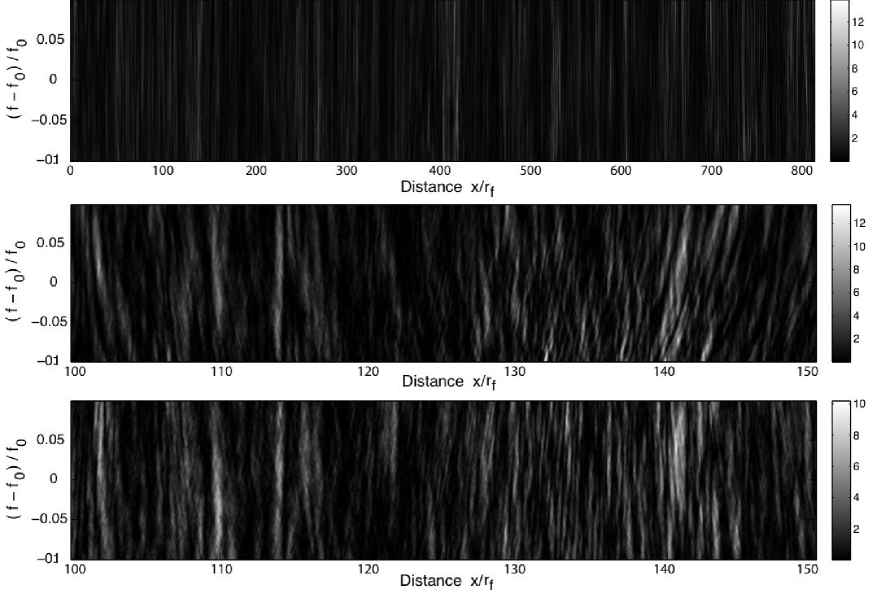
Figure 1.— Dynamic spectra for $m_{b}^{2}=10$: (a) the top panel is the full dispersive simulation; (b) the middle panel is an expanded section of the top panel; (c) the bottom panel is the same as (b) except the simulation is run without dispersion. In each case the abscissa is scaled with respect to the Fresnel scale $r_{\text{f}}$, (about $3.2\times 10^{5}$ km for a typical pulsar). If converted to a time axis using a velocity of 100 km/s, the full window corresponds to about a month of observation.

We have addressed this problem using simulated dynamic spectra which are much longer than a typical observation. A 16384 x 2048 (x,y) window was simulated and the center slice $y=y_{0}$ of length 16384 was extracted. Then the simulation was repeated at 128 different frequencies, building up a dynamic spectrum of 16384 x 128 (x,f) from the central slices of each window. An example is shown in Figure 1a. In this particular simulation $m_{b}^{2}=10$ and the abscissa has been scaled by $r_{\text{f}}$ = 20 samples. The spatial scales derived from the measured covariance functions of electric field and intensity are $s_{0}=0.20\ r_{\text{f}}$, $s_{\text{dif}}=0.22\ r_{\text{f}}$ and $s_{\text{ref}}=5.5\ r_{\text{f}}$ (estimation of spatial scales will be discussed in detail in the following section). The theoretical scales are $0.215\ r_{\text{f}}$, $0.215\ r_{\text{f}}$ and $4.65\ r_{\text{f}}$ respectively. Thus $s_{\text{dif}}/dx=4.4$ so the smaller scales are well-sampled, and $L_{y}/s_{\text{ref}}=19$ so the largest scales fit easily in the window. For a typical pulsar at a distance of 200 pc with a scattering screen at 100 pc observed at 1.4 GHz the Fresnel scale $r_{\text{f}}=3.2\times 10^{5}$ km. The drift time for $r_{\text{f}}$ at 100 km/s would be about 1 hr, so the simulated window of 16384 samples corresponds to about a month of continuous observations. The same sampling was used for $0<m_{b}^{2}\leq 30$ but for $m_{b}^{2}>30$ we used 32768 x 4096 x 256.

The expanded window plotted in Figure 1(b) shows both the diffractive and refractive structures more clearly. The expanded view also shows that the structure is often tilted or even curved. This phenomenon, which will be discussed later, is primarily due to dispersion. This is demonstrated by the bottom panel, Figure 1(c), which shows the dynamic spectrum of the same phase screen without dispersion.

Observers estimate the temporal and frequency scales of the observations by calculating the autocovariance of the dynamic spectrum. Of course this averages the temporal scale over the frequency range in the dynamic spectrum, but the temporal scale varies almost linearly with frequency and the fractional bandwidth is usually less than 25% so this is not a significant bias. We computed the two dimensional autocovariance of the entire dynamic spectrum shown in Figure 1 (a). Cuts through this autocovariance are shown as solid lines on Figure 2. In the left panel $\Gamma_{\cal I}(s)$ is shown with a logarithmic abscissa so that one may see both the spatial scales clearly. The frequency correlation $\Gamma_{\cal I}(\Delta\text{f})$ is shown in the right panel. The fractional bandwidth $\delta\nu/\text{f}_{0}$ = 0.027, considerably smaller than the $(s_{0}/r_{\text{f}})^{2}=0.046$ expected theoretically. The diffractive scale is well-estimated because there are $(L_{x}/s_{\text{dif}})*(B/\delta\nu)=1.7\times 10^{4}$ degrees of freedom in the dynamic spectrum (here $B$ is the width of the dynamic spectrum in frequency). However the refractive scale is broadband and much larger, so there are only $(L_{x}/s_{\text{ref}})*1=136$ degrees of freedom in the dynamic spectrum, and the refractive component is much less stable. To improve our estimate of the refractive process we have computed the autocovariance of the entire 16384 x 2048 window at the center frequency $\text{f}_{0}$. This provides $(L_{x}/s_{\text{dif}})*(L_{y}/s_{\text{dif}})=2330$ degrees of freedom and a much better estimate of the refractive component.

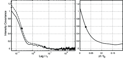
Figure 2.— Estimates of $\Gamma_{\cal I}(s)$ (left panel) and $\Gamma_{\cal I}(\Delta\text{f})$ (right panel) from the dynamic spectrum displayed in Figure 1(a) are shown as solid lines. In the left panel an estimate of $\Gamma_{\cal I}(s)$ calculated from the entire simulation plane at $\text{f}_{0}$ is also shown as a dashed line. It provides a more stable estimate of $\Gamma_{\cal I}(s)$ than does the dynamic spectrum alone, because there are more refractive scales in the entire simulation plane. The widths $s_{\text{dif}}$ and $\delta\nu/\text{f}_{0}$ are marked as solid circles. The abscissa in this panel is displayed with log scaling so both diffractive and refractive scales can be observed clearly. The zero points, which are not on the log abscissa, are marked as diamonds on the left axis.

We have broken the full dynamic spectrum into 128 blocks, each of length approximately $s_{\text{ref}}$, which corresponds to about 6.4 hrs of observation, and estimated the autocovariance in time and in frequency for each block. In each block there are 215 degrees of freedom in the diffractive process. From these we derived the spatial (temporal) and frequency scales for each block, by fitting a theoretical model to the appropriate autocovariance of each block. The results are shown in Figure 3. The error bars shown on Figure 3 are $\pm 2\sigma$ as determined from the least squares fitting process.

The theoretical model for the spatial correlation is $\Gamma_{\cal I}(s)=\exp(-(s/s_{\text{dif}})^{5/3})$, which is the known asymptotic form in strong scattering. The asymptotic forms for $\Gamma_{\cal I}(\Delta\text{f})$ are similar in shape but do not have a simple closed form (Coles et al., 1995b). We found that an exponential $\Gamma_{\cal I}(\Delta\text{f})=\exp(-|\ln(2)\Delta\text{f}/\delta\nu|)$ gave a reasonable match to the theory and also to the overall average, so we used this model in the block fits. A gaussian model would give a significantly different fit.

The spatial scale is shown in the upper panel of Figure 3. The overall $s_{\text{dif}}$ normalized to $s_{0}$ is 1.02, the weighted mean of the 128 blocks, normalized the same way, is 0.89. The unweighted rms of the 128 blocks is 47% but the standard deviation computed from the error bars estimated by the fitting process is only 9%, i.e. these error bars underestimate the actual error by a factor of five. The frequency scale $\delta\nu$ normalized to $\text{f}_{0}$ is shown in the lower panel of Figure 3. The overall $\delta\nu/\text{f}_{0}$ is 0.027, whereas the weighted mean of the 128 blocks is 0.017 so the mean of the blocks is only 63% of the overall average. The unweighted rms of the blocks is 84% of the weighted mean but the standard deviation computed from the error bars is only 6%. Again the error bars seriously underestimate the actual variation of the block estimates.

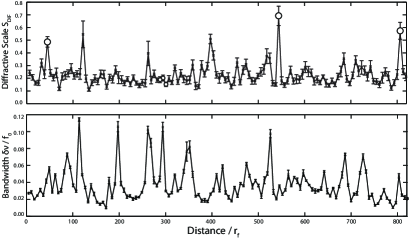
Figure 3.— Upper panel, apparent diffractive scale $s_{\text{dif}}$ measured on blocks of length $s_{\text{ref}}$. Lower panel, apparent diffractive bandwidth $\delta\nu$ measured on the same blocks. The points marked with open circles are discussed below as examples of “good” and “bad” fits.

Since the analysis shown in Figure 3 is typical of that used by observers, it is disappointing to find that the error bars determined by a least squares fit are so unreliable in both time (space) scale and bandwidth. Observers have noted this effect and Cordes (1986) has suggested that the error bars should be computed with the number of degrees of freedom reduced by a factor of 25 to 100. In the simulation shown reducing the number of degrees of freedom from 215 to 2 would indeed match the estimated error to the observed rms variation. However the variations do not have a Gaussian distribution, as demonstrated by the obvious “spikes”. So there is a finite possibility of a much larger error.

The spikes in time scale and bandwidth are not correlated. The cause of the spikes is not obvious on an inspection of the block correlations. In Figure 4 we show six examples of the time scale fits. The top three panels are from the spikes at blocks 7, 85, and 126 which are marked with large open circles in Figure 3. The lower three panels are normal fits at samples 46, 47 and 48 which are marked with small open circles in Figure 3. Although the top three panels represent huge errors, this is not apparent in the fit. Since this is a very important issue for observers, we have reanalyzed the data in blocks of half and twice the refractive scale. The results are provided in Table 1. As expected, the reported errors decrease with longer block lengths. However the rms is rather stable. This suggests that the rms is not caused by statistical errors in the fit, but by the refractive fluctuations. The downwards bias of the mean becomes worse with shorter blocks. Perhaps more important, the frequency of spikes is roughly independent of block length.

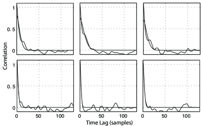
Figure 4.— Least squares fit to correlation functions from six blocks. The top three panels are from spikes at blocks 7, 85, and 126. The lower three panels are from more typical blocks 46, 47 and 48. The noisy lines are the estimated covariances and the smooth lines are the best fit theoretical models.

It is well known that least squares fits to correlation functions violate the normal assumptions that the errors (i.e. the deviations of the observations from the model) are independent and have equal variance. So we re-estimated the spatial scale by doing a least squares fit to the Fourier transform of the correlation function. The advantage of this is that the errors in the Fourier transform are independent and their variance is known, so it can be corrected in a weighted fit. We used exactly the same correlation model, but fit its Fourier transform to the Fourier transform of the correlation. The resulting spatial (time) scale is shown in Figure 5.

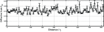
Figure 5.— Diffractive spatial (temporal) scale obtained by a weighted least squares fit in the frequency domain.

One can see by eye that the spikes have completely disappeared, the rms is considerably smaller, but the mean is also lower. These parameters are also given in Table 1. The weighted mean has decreased to 72% of the true value. The rms has decreased by a factor of three, but the error bars are still far below the rms.

Table 1Diffractive Scale (normalized by $s_{0}$)

fit:	block	wtd mean	rms	error bar
cov	$2s_{\text{ref}}$	0.99	43%	7%
	$s_{\text{ref}}$	0.89	47%	9%
	$s_{\text{ref}}/2$	0.78	53%	12%
spec	$s_{\text{ref}}$	0.72	18%	3%

The same fits shown in Figure 4 are displayed in the frequency domain in Figure 6. One can see that there is a low frequency excess in the top panels, which gave rise to spikes when fit in the time domain, but these do not significantly distort the fit in the frequency domain because the optimal weighting favors the higher frequencies. Thus fitting the power spectrum is strongly recommended. It provides a much better estimator of the spatial (temporal) scale, although users will have to correct for a downwards bias of the order of 30% and the error bars will not be more reliable. Fitting in the spectral domain would be particularly valuable when one is analyzing the effect of orbital motion on scintillation of a binary pulsar, or when one is attempting to measure the annual modulation in time scale due to the Earth’s velocity. It is clear that in all cases observers should be extremely cautious about the errors estimated from data blocks whose length is less than the refractive scale.

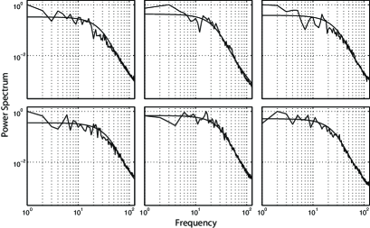
Figure 6.— Weighted least squares fit to the block power spectra. The noisy lines are the power spectra and the smooth lines are the best fit theoretical model. The blocks are the same as those shown in Figure 4.

We have not attempted to fit the frequency scale $\delta\nu$ in the Fourier domain, but we expect that it would also be better fit in this way. The theoretical model for $\Gamma_{\cal I}(\Delta\text{f})$ is demonstrably inadequate because the value of $\delta\nu$ measured from the simulation shown is only 59% of that expected theoretically. The theory applicable to moderately strong scattering has been worked out (Codona et al., 1986), but it has not been applied to interstellar scintillation. This should be done, but is beyond the scope of this paper. Observers have also noted this effect and Gupta et al. (1994) have given a heuristic model which explains the reduction in $\delta\nu$ in terms of refractive modulation of the diffractive scintillation, combined with the plasma dispersion. This model agrees approximately with the simulations. The bias changes slowly with increasing strength of scattering as will be shown later.

We do not understand why the fluctuations in spatial scale are not correlated with those in bandwidth. This effect has been considered by Gupta et al, (1994) who suggested that refractive variations that tilt the spatial structure should change the bandwidth but not the scale. This is clearly not true of our simulations, both the bandwidth and the spatial scale are highly variable. These variations have also been observed in an extensive monitoring of ISS from a set of 18 pulsars by Bhat et al. (1999). They estimated the frequency and time scales fitting the covariance functions as we have done, but with a Gaussian model. We believe that the variability is due to the fact that some 20% of the variance is caused by refractive effects which are ignored, but which significantly modulate the diffractive effects. The various heuristic models employed by observers are useful, but this problem would benefit from further theoretical work based on Codona et al. (1986) and further simulations. In particular it would be very useful to extrapolate our results to stronger scintillation where the bias should decrease.

5. Secondary Spectra

It has been noticed for decades (Ewing et al. 1970; Roberts & Ables 1982), that dynamic spectra often show “criss-cross” structures. These structures, which are easily visible in Figure 1(b), are responsible for the “parabolic arcs” discovered by Stinebring et al. (2001) and discussed by Cordes et al. (2006), which are seen in the “secondary spectrum.” The secondary spectrum, which is the two-dimensional power spectrum of the dynamic spectrum and has been called the delay-Doppler spectrum, is shown in Figure 7. Here the delay axis has been scaled to ns assuming the center frequency is 1.4 GHz. This scaling will be continued throughout. The Doppler axis is scaled by $r_{\text{f}}/V_{\text{eff}}$. With the values used earlier the Doppler range would be $\pm 3$ mHz. An arc is visible in Figure 7, but it is quite symmetric and not sharply defined. Most observed arcs are more clearly defined and they are often quite asymmetric. It is known that the arcs would be sharper in weaker scintillation or if the scattering were anisotropic (Cordes et al. 2006) and this is a strong argument that interstellar turbulence is often anisotropic. However it has not been understood exactly why observations often show asymmetric arcs. It has been assumed that this is due, in some way, to refraction, but it has been unclear whether this requires a discrete refracting structure, or whether the refraction that occurs naturally due to the low frequency part of the turbulent spectrum is sufficient. To test this question we have broken the full dynamic spectrum into smaller blocks, typical of the observation duration (as was done in calculating the time and frequency scales in Figure 3). The results, which are shown in Figure 8, show exactly the characteristics of the observations. The arcs are sometimes quite asymmetric and the orientation of the asymmetry reverses on a time scale considerably longer than the refractive time scale. Evidently this resolves the question of whether such asymmetric secondary spectra are due to discrete deterministic structures or to refractive components of a turbulent spectrum - they can be caused by a continuous turbulent spectrum, but the scales involved are larger than the refractive scale.

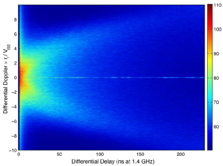
Figure 7.— The delay-Doppler spectrum computed from the dynamic spectrum shown in Figure 1 (a). The brightness scale is dB = 10log₁₀(power).

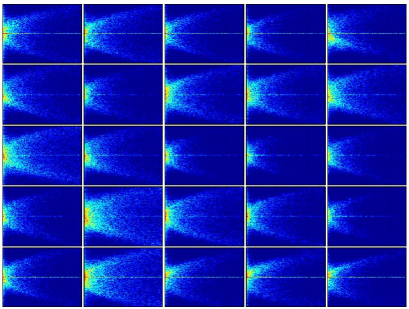
Figure 8.— Delay-Doppler distributions computed from 25 blocks of the dynamic spectrum shown in Figure 1(a). Time increases from the top left, first to the right, then down, ending at bottom right. Each panel has the same axes as Figure 7.

When the same phase screen is simulated without dispersion the dynamic spectrum, which is plotted in Figure 1(c), shows criss-cross structures but very little tilt. The average secondary spectrum is very similar to that shown in Figure 7, but the secondary spectra of shorter blocks, which are shown in Figure 9, do not show the time varying asymmetry characteristic of the dispersive simulation shown in Figure 8. Thus there can be no doubt that the phenomenon of tilted bands in dynamic spectra is not caused solely by refraction, but by dispersion and refraction. With this insight it is relatively simple to describe the phenomenon analytically. The physical difference can be explained intuitively. Large scale refraction will tilt an entire angular spectrum regardless of dispersion. However it will tilt to the minimum phase delay position (due to Fermat’s Principle). The secondary spectrum is caused by interference of scattered waves with different group delay and different Doppler shift. In a non-dispersive problem the group delay is equal to the phase delay so a refractive shift of the entire angular spectrum has no effect on the secondary spectrum. When the medium is dispersive the phase delay is the negative of the group delay, so the position of minimum phase delay is not the position of minimum group delay. Indeed it is a local maximum of group delay. In this case a refractive tilt has a dramatic effect on the parabolic arc. A rough analysis is given below.

Figure 9.— Delay-Doppler distributions computed from 25 blocks of the non-dispersive dynamic spectrum shown in Figure 1(c).

We assume (without loss of generality) a thin screen half way between a pulsar and the observer. The arcs are caused by the interference of a wave scattered at an angle $\delta\theta$ in the direction of the velocity and an unscattered wave. The two waves interfere with differential Doppler shifts $\delta f_{d}=2V\delta\theta/\lambda$ and differential delays $\delta\tau_{d}=z\delta\theta^{2}/c$ where z is the distance from the screen to the observer. It is useful to normalize the parameters with respect to the rms scattering angle $\theta_{0}$, i.e. $f_{d0}=2V\theta_{0}/\lambda$ and $\tau_{d0}=z\theta_{0}^{2}/c$. Then $\delta\tau_{d}/\tau_{d0}=(\delta f_{d}/f_{d0})^{2}$ defines the parabolic arc in normalized form.

Now we consider the effect of a phase gradient $\nabla\phi_{*}$ in the screen. It will tilt the angular spectrum seen by the observer by an angle $\theta_{*}=\nabla\phi_{*}/2k$. If the gradient is perpendicular to the velocity then it will have no effect on the arc. Thus we consider only the gradient in the direction of the velocity. The group delay is given by $\tau_{g}(\theta)=z\theta^{2}/c\mp z\theta\nabla\phi_{*}/\omega$ in nondispersive (top sign) and dispersive (bottom sign) cases. The differential Doppler between an unscattered wave arriving at angle $\theta_{*}$ and a scattered wave arriving at angle $\theta_{*}+\delta\theta$ is unchanged by the phase gradient. The differential delay is more complex. In the non-dispersive case we have $\delta\tau_{d}=z\delta\theta^{2}/c$, i.e. the arcs are unaffected by a phase gradient, at least to first order. However in the dispersive case we have $\delta\tau_{d}=z(\delta\theta^{2}+4\theta_{*}\delta\theta)/c$. Putting this in normalized form we have $\delta\tau_{d}/\tau_{d0}=(\delta f_{d}/f_{d0}+2\theta_{*}/\theta_{0})^{2}-(2\theta_{*}/\theta_{0})^{2}$. The apex of the arc is shifted in Doppler by $(2\theta_{*}/\theta_{0})f_{d0}$ and in delay by $(2\theta_{*}/\theta_{0})^{2}\tau_{d0}$. Thus, if the phase gradient shifts the entire angular spectrum by an amount comparable with the rms scattering angle $\theta_{0}$, then the shift in the apex of the parabola should be detectable in a dispersive medium. This analysis shows why tilted arcs are observed in dispersive cases and not in non-dispersive cases. It also agrees with earlier rough analyses of the slope of tilted structures in the dynamic spectrum (Shishov 1974; Hewish 1980; Gupta et al. 1994). However, it is difficult to use these expressions quantitatively to estimate the electron density gradients in the IISM because the arcs are not always very distinct (as in the case simulated). To do this one would need to model the entire secondary spectrum including the effects of gradients both parallel and perpendicular to the velocity.

6. TIME OF ARRIVAL FLUCTUATIONS

6.1. Pulse Shape

The simulated electric field $E(x,y,f)$ allows one to calculate the pulse $I(x,y,t)=|F_{\text{f}}\{E(x,y,f)\}|^{2}$ at each pixel. Here $F_{\text{f}}$ is the Fourier transform operating on coordinate f. Thus the simulation provides a direct calculation of the pulse shape, including the arrival time variations. In the simulation the mean electron density over the simulation window is zero, but at any given position there is “dispersion delay” and it fluctuates with position. In addition the pulse shape changes on both the diffractive and refractive scales. This is shown in Figure 10. Here the pulse power is shown on a $\log_{10}$ scale over a 40 dB dynamic range. The phase screen delay at $f_{0}$ is overplotted on Figure 10 as a white line. The screen delay is taken as the group delay of the phase screen, which is the negative of the phase delay for a plasma. In the top panel one can see that the peak of the pulse power tracks the slow variation due to dispersion measure. In the bottom panel one can see the much finer scale variation due to diffractive and refractive scattering.

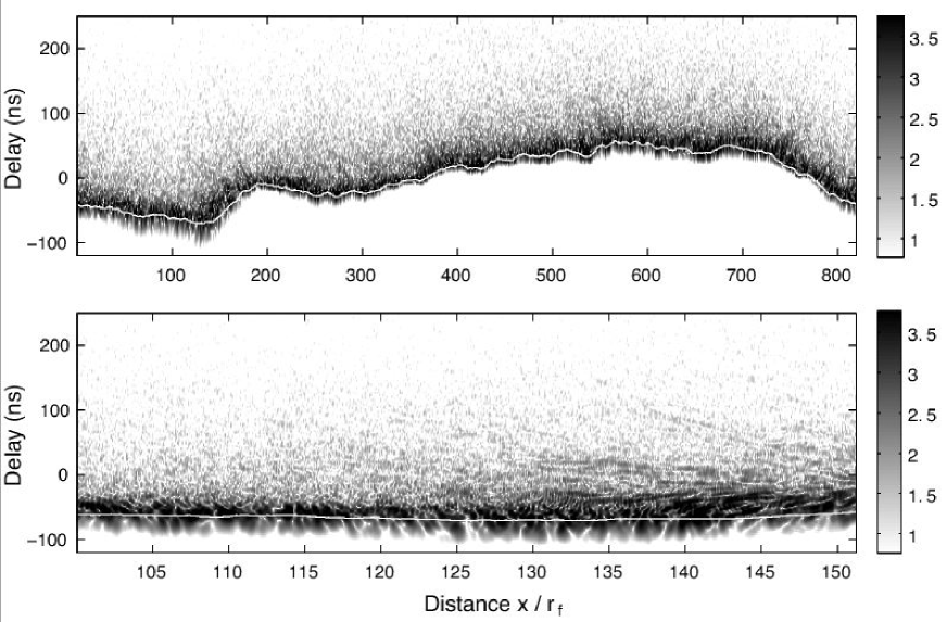
Figure 10.— Pulse shape vs position. The intensity is log10(power). The lower panel is an expanded section of the upper one. The white line is the group delay through the screen at the same transverse location as the intensity “measurement”.

The average pulse shape would be dominated by the dispersion measure variations. However the scattered pulses can be aligned with respect to the dispersion delay in the screen itself. With this alignment all the delay variations are due to propagation from the screen to the observer. The average pulse-shape, which is the expected quasi-exponential, is shown in Figure 11. Note that this figure has a log ordinate, so an exponential pulse would drop linearly with delay. In order to display the leading edge of the pulse with low sidelobes we used a Blackman window in the Fourier transform for this display. One can see that the pulse tail does not drop nearly as fast as the exponential, which would be characteristic of a Gaussian angular spectrum. This is because the actual angular spectrum falls more slowly than a Gaussian at large angles. It is easily shown that at high angles $B(\theta)\propto\theta^{-(\alpha+2)}$, so $I(t)\propto t^{-(\alpha+2)/2}$. The asymptotic diffractive theory is overplotted as a dashed line. The theoretical curve was scaled up by a factor of 1.5 to allow for rounding of the peak by the Blackman window. It is clear that the long term average, when corrected for dispersion measure fluctuations, agrees very well with the simple diffractive theory.

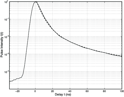
Figure 11.— Average pulse shape I(t), corrected for dispersion measure variations in the screen. The finite rise time is due to the bandwidth limit and the spectral window. The Blackman window is used because it provides very low sidelobes but it is considerably broader than a rectangular window. The dashed line is from the simple diffractive theory. It has been shifted up by a factor of 1.5 to allow for rounding of the peak by the Blackman window.

The diffractive effect is not to spread each pulse into a quasi-exponential, rather to break the pulse into subpulses. This is shown in a very expanded view in Figure 12. It is only the superposition of all the pulses that is a continuous quasi-exponential. The width of the fragments of each pulse appears to be the resolution of the Fourier transform i.e. the inverse of the bandwidth. One never observes such breakup of the pulse shape in pulsars because the intrinsic pulse width is always much larger than the inverse of the bandwidth. It might be observable in giant pulses with coherent de-dispersion (e.g. Hankins et al., 2003).

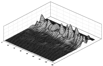
Figure 12.— Expanded view of the pulse shape. Pulse delay runs downwards to the left. The total delay shown (80 ns) is comparable with the range shown on Figure 11. Observing time runs downwards to the right. Pulse power is vertical. The period displayed is the drift time for 8 $r_{\text{f}}$ or about 1.2 refractive time scales.

6.2. Pulse Centroid

Diffractive scattering also causes the centroid of the pulse to shift, and this effect is observable. Indeed it may be an important source of timing noise in some pulsars (Foster & Cordes 1990). The centroid is shown in the top panel of Figure 13 with the phase screen delay marked as a black line. One can see that the centroid of the pulse does not follow the screen delay as well in regions of high gradient in screen delay. This difference is much weaker in the non-dispersive case, which is shown in the lower panel. Here, of course, the screen delay plotted is the phase delay and it has the opposite sign of the group delay in the upper panel. Clearly a steep gradient in either case leads to increased refraction but the effect of this refraction on the delay is much greater in the dispersive case.

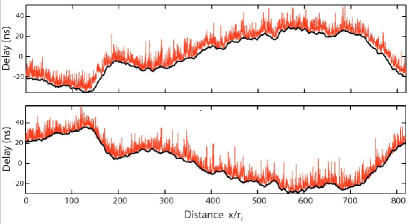
Figure 13.— Pulse centroid vs position. Top panel dispersive, bottom panel non-dispersive. The black line is the mean delay of the screen simulated at the observer’s position.

It has been known for some time that scattering causes fluctuation in pulse arrival times, and that this fluctuation is anticorrelated with pulse power. This has been discussed theoretically (Blandford & Narayan 1985) and observed (Lestrade et al. 1998). Theory and observations were discussed in terms of a refractive mechanism applied to observations which were averaged over many diffractive time scales. The anti-correlation also exists at diffractive scales, as can be seen in Figure 14 panels a and b. Here the first 50 $r_{\text{f}}$ of the simulation shown in Figure 13 have been expanded to show the diffractive structure. The centroid corrected for the screen delay $T_{c}$ is shown in the top panel. In the middle panel we show the total pulse flux density $P_{T}$. The anti-correlation is evident both at $s_{\text{dif}}=0.22r_{\text{f}}$ and at $s_{\text{ref}}=5.5r_{\text{f}}$. The correlation is significantly higher between $T_{c}$ and $1/\sqrt{P_{T}}$ as apparent in Figure 14c. Here the raw cross correlation is 73%, and it rises to 83% if both series are low pass filtered to remove all scales larger than the refractive scale.

The anti-correlation between TOA and flux at the diffractive scale has not been discussed theoretically, but one can see the mechanism involved by examining the shape of successive pulses on the diffractive time scale as shown in Figure 12. Evidently the pulse shape changes significantly on the diffractive time scale, so the instantaneous angular spectrum must also vary significantly on that time scale. When the angular spectrum broadens the pulse broadens, and the flux drops correspondingly. However the pulse broadening is one-sided, it always increases the delay, so the delay of the centroid increases when the flux drops and we see this as an anti-correlation.

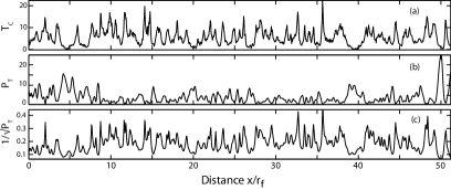
Figure 14.— The centroid corrected for dispersion measure $T_{c}$ (top panel). Total pulse power $P_{T}$ (middle panel). $1/\sqrt{P_{T}}$ (bottom panel). The cross correlation of the top and bottom figures is 73%. It rises to 83% when scales larger than 28 $r_{\text{f}}$ are filtered out. Here the first 50 $r_{\text{f}}$ of the 800 $r_{\text{f}}$ in the simulation have been expanded so the diffractive fluctuations can be seen clearly.

One can see an interesting structure centered near $x=40r_{\text{f}}$, which very much resembles a structure observed by Cognard et al. [1993] who called it an extreme scattering event and attributed it to a discrete cloud of plasma. Our simulation shows that such events can occur naturally in Kolmogorov turbulence and this is confirmed by recent simulations very similar to ours [Hamidouche and Lestrade, 2007].

The $T_{c}$ fluctuations show a larger scale component (in addition to diffractive and refractive components) which is not correlated with $1/\sqrt{P_{T}}$. It does show a strong correlation with the magnitude of the gradient of the screen phase. This component is refractive but of larger scale than the refractive intensity fluctuations. Here the phase is essentially linear over the scattering disc, so we use a plane wave approximation. A phase gradient $\nabla_{x}\phi$ will cause an angular shift $\Delta\theta_{x}=\nabla_{x}\phi/k$. This will displace the pattern by $z\Delta\theta_{x}=z\nabla_{x}\phi/k$ and thus cause a phase difference between the observed phase and the phase in the screen of $\Delta\phi=z\Delta\theta_{x}\nabla_{x}\phi=(r_{\text{f}}\nabla_{x}\phi)^{2}$. This causes a TOA error of $\Delta\phi/\omega=(r_{\text{f}}\nabla_{x}\phi)^{2}/\omega$. There is also an incremental free space delay of half this TOA error, i.e. $0.5*\Delta\theta_{x}^{2}z/c=0.5*(r_{\text{f}}\nabla_{x}\phi)^{2}/\omega$. For a non-dispersive medium the free space delay partially cancels the refractive component (an expression of Fermat’s principle) and the cross correlation between $T_{c}$ and $(r_{\text{f}}\nabla\phi)^{2}/\omega$ would be negative. For dispersive medium the free space delay adds to the refractive component and the cross correlation is positive and larger. This crude analysis shows why a correlation between $T_{c}$ and $(r_{\text{f}}\nabla\phi)^{2}/\omega$ should be expected and, because the $\nabla_{y}$ is ignored, why this correlation should not reach 100%. We will refer to this larger scale as the dispersive scale because it is stronger and positive in a dispersive simulation. The correlation can be seen clearly in Figure 15, where both $T_{c}$ and $\nabla\phi$ have been lowpass filtered to remove all the diffractive and refractive fluctuations. In this example the correlation coefficient for the dispersive case is 70% and for the non-dispersive case it is -37%.

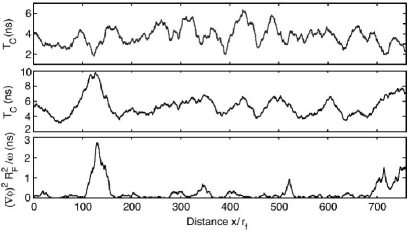
Figure 15.— A comparison of the corrected centroid from Figure 14, smoothed over 28 $r_{\text{f}}$ to eliminate both refractive and diffractive fluctuations, with $(r_{\text{f}}\nabla_{x}\phi)^{2}/\omega$ where $\nabla_{x}\phi$ has the same smoothing. (a) top panel the scattering medium is non dispersive; (b) middle panel the medium has the plasma dispersion; (c) the term $(r_{\text{f}}\nabla_{x}\phi)^{2}/\omega$. The cross correlation of the middle and bottom panels is 70%. The cross correlation of the top and bottom panels is -37%.

6.3. Correction of TOA Variation

Since the TOA variations are highly correlated with intensity one can use the measured intensity to remove the correlated components of the TOA variation. We have done this in two steps. First we have reduced the correlation with $1/\sqrt{P_{T}}$ to zero by subtracting a constant times $1/\sqrt{P_{T}}$ from $T_{c}$, creating $T_{cc}$. This reduced the variance in $T_{c}$ by more than a factor of two. We then reduced the correlation with $(r_{\text{f}}\nabla\phi)^{2}/\omega$ to zero in the same way, creating a $T_{ccc}$. This reduced the variance by another 20%. The three stages $T_{c}$, $T_{cc}$, and $T_{ccc}$ are shown in Figure 16 from top to bottom. Of course in practice our estimates of $1/\sqrt{P_{T}}$ and $|d(DM)/dx|$ will have error so the correction process will add some white noise, but in practice these errors are quite small compared with the white noise in $T_{c}$ so the added white noise is negligible.

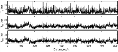
Figure 16.— The pulse centroid corrected for: (top panel) dispersion measure fluctuations; (middle panel) intensity scintillation; (bottom panel) gradient of dispersion measure. The scales are the same in the three panels. One can see the effect of removing correlated components clearly.

7. Correction of TOA Fluctuations in Practice

We have tested the correction process using observations of J0437$-$4715, a powerful nearby pulsar, at 685 MHz, using the Parkes radio telescope with the CPSR2 coherent de-disperser backend. The observations are similar to those described by Verbiest et al. (2008). These observations were made during a period of particularly heavy sampling between April 22, 2006 and June 11, 2007. There were observations on 62 days with an average of 140 minutes per day. The total IF bandwidth is 64 MHz. Pulse arrival times were estimated on, roughly, 5 minute subintegrations, and the signal to noise ratio (SN) was also estimated. The Verbiest et al. (2008) timing model was used. The only timing parameter fitted was the pulse phase. Observations made simultaneously at 3 GHz were used to estimate the dispersion. The integrated pulse power was not flux calibrated but it is believed that the 50 cm receiver noise is quite stable so the signal to noise ratio is proportional to the pulse flux. As this source is nearby the dispersion is relatively small, even at 685 MHz, but it is not negligible. The autocovariance of $1/\sqrt{SN}$ is shown in the left panel of Figure 17. It shows a quasi-exponential covariance with a time scale of about 20 min (which is the diffractive scale) and very little white noise (which would appear as a delta function at the origin). The autocovariance of the timing residuals corrected for dispersion is shown in the right panel of Figure 17. This covariance shows a clear white noise component and an exponential component with a time scale of about 30 min. This is not significantly different from the diffractive scale and is undoubtedly associated with the diffractive intensity variations. The white noise carries about the same variance as the 30 min variations.

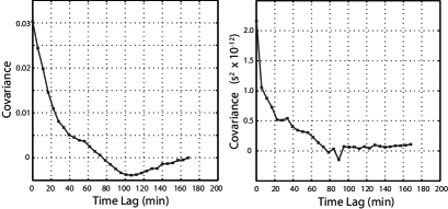
Figure 17.— Autocovariances of $1/\sqrt{SN}$ (left panel) and TOA residuals (right panel) for pulsar J0437$-$4715 at 685 MHz.

It should be noted that the rms white noise in these observations, about 1 $\mu$s, is much larger than the white noise in the normal observations of the Parkes Pulsar Timing Array (PPTA) for several reasons. The basic PPTA timing is done at 1400 MHz where the effects of the ISM are much smaller, with a much broader bandwidth and a much longer integration time, so the receiver noise is much lower.

The cross correlation of the residuals with $1/\sqrt{SN}$ is shown in Figure 18 before and after the scattering correction. One can see that in advance of the scattering correction the correlation (shown dotted) was about 50%. If one corrects for the white noise component in the residuals the correlation of the diffractive component is about 70% as in the simulations. After the scattering correction the correlation (shown solid) is zero as expected. The scattering correction reduces the total variance of the residuals by about 25%. However one can see that the cross correlation persists as a negative component away from the origin. This could perhaps be removed using a more sophisticated removal. Rather than subtracting a constant times $1/\sqrt{SN}$ one could subtract the reference after being filtered with an FIR filter, as would be done in an adaptive echo canceller.

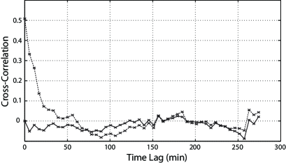
Figure 18.— Cross correlation of TOA residuals with $1/\sqrt{SN}$ for pulsar J0437$-$4715 at 685 MHz. The trace shown dotted is before correction of the residuals for scattering and the trace shown solid is after this correction.

It has been noted [Verbiest et al, 2009] that the errors in the residuals of J0437$-$4715 do not behave like white noise. In particular when residuals sampled at 5 minute intervals are averaged the error on the average does not shrink like the square root of the number of residuals averaged. This is clearly because half the variance is carried in the diffractive component which has a correlation time considerably longer than 5 minutes.

In this pulsar we are able to observe and correct diffractive fluctuations in the TOAs. The refractive fluctuations were negligible but it seems likely that they too could have been corrected the same way. We attempted to analyze the refractive scattering contribution of the pulsar J1939$+$ 2134, as was done by Lestrade et al. [1998] however the pulsar is not sampled adequately in the normal PPTA observations to resolve the 2.5 day time scale of the refractive scintillation.

8. A HEURISTIC MODEL OF TOA VARIATION

It would be very useful to be able to predict the TOA variations discussed above for a given pulsar at a given frequency. Since we lack an analytical theory, we have created a heuristic model with which we can scale the results of simulations to match the observing parameters. First we ran simulations over the range of strengths of scattering ($m_{b}^{2}$) accessible to our computing platforms: 3, 5, 10, 20, 30, 60, and 100. Then we compared the behavior of the parameters for which we have theoretical scaling models, with the simulations. This comparison validates both the simulations and the scaling models.

The fundamental spatial scales are: the $e^{-0.5}$ scale of the electric field ($s_{0}$); the diffractive $e^{-1}$ scale of intensity ($s_{\text{dif}}$); and the refractive $e^{-1}$ scale of intensity ($s_{\text{ref}}$). The scales of intensity were measured at their half power points, i.e. $\Gamma=(3m^{2}-1)/4$ and $(m^{2}-1)/4$, and then corrected to the $e^{-1}$ values using the theoretical curve shape. The scale of the field is measured from the autocovariance of the field at $e^{-0.5}$. The results are plotted vs $m_{b}^{2}$ in Figure 19 as symbols with error bars. The error bars are derived from multiple simulations. For a given $m_{b}^{2}$ we can use equation (3) to find $s_{0}$. This expression, which is valid in any strength of scattering, is plotted as a solid line and agrees well with the simulations. The strong scattering approximation for diffractive scale $s_{\text{dif}}=s_{0}$ agrees less well but improves in stronger scattering. The strong scattering approximation for refractive scale $s_{\text{ref}}=r_{\text{f}}^{2}/s_{0}$, which is also plotted as a solid line, has weak agreement with the simulations. A heuristic expression for $s_{\text{ref}}$ derived from numerical solutions to the moment equations (Goodman and Narayan, 2006), which is plotted as dashed line, agrees much better. It is reassuring that the numerical solution agrees with the simulations for $s_{\text{ref}}$.

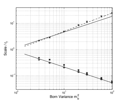
Figure 19.— Spatial scales from the simulations. The scales $s_{\text{dif}}$ (star), $s_{\text{ref}}$ (cross) and $s_{0}$ (circle) are normalized to $r_{\text{f}}$. The error bars are derived from multiple simulations. The theoretical expressions drawn as solid lines fit $s_{0}$ quite well, $s_{\text{dif}}$ less well, and $s_{\text{ref}}$ weakly. An empirical expression for $s_{\text{ref}}$ (Goodman and Narayan, 2006) shown as a dashed line, fits well.

The intensity variance is a fundamental parameter, but theoretical expressions are difficult to derive. We have plotted $m^{2}-1$ as symbols with error bars in Figure 20. An asymptotic expression for large $m_{b}^{2}$ is plotted as a dashed line (Prokhorov et al. 1975). An empirical expression derived from numerical calculations is plotted as a solid line (Goodman and Narayan, 2006). One can see that the asymptotic expression converges very slowly, whereas the empirical expression is quite good throughout the simulated range. Observers should be cautious using the asymptotic expression because it evidently does not become accurate until $m_{b}^{2}>100$ and for such strong scattering the inner scale is likely to become important (increasing the variance). Thus one should use the asymptotic approximation only when one is prepared to make a correction for the inner scale.

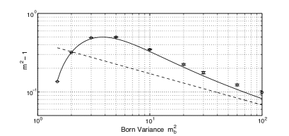
Figure 20.— Intensity variance $m^{2}-1$ from the simulations. The error bars are derived from multiple simulations. The empirical expression (Goodman and Narayan, 2006) drawn as a solid line fits quite well. The asymptotic expression (Prokhorov et al., 1975) drawn as a dashed line converges very slowly.

The fundamental time scale is the pulse width. A theoretical expression can be derived using $s_{0}$ to obtain $\theta_{0}=1/ks_{0}$ and then $t_{0}=\theta_{0}^{2}z/c$. The measured pulse width ($t_{0obs}$) is obtained from the measured bandwidth $\delta\nu$ by $t_{0obs}=1/2\pi\delta\nu$. The theoretical pulse width $t_{0}$ and the measured TOA variations, normalized to the measured pulse width $t_{0obs}$, are displayed in Figure 21. The ratio $t_{0}/t_{0obs}$ is shown as square boxes. This ratio should be unity of course, but the dashed line through the data, which is given by $t_{0}/t_{0obs}=0.43(m_{b}^{2})^{0.11}$, is clearly a good approximation. We note that at $m_{b}^{2}=10$ the observed pulse width is twice the theoretical width. This was discussed in section 4 where we noted that the observed $\delta\nu$ is only half that theoretically predicted. This discrepancy decreases very slowly with increasing $m_{b}^{2}$ and probably becomes asymptotic to unity for $m_{b}^{2}>>100$. If this expression is used then $t_{0obs}$ scales with $\lambda$ according to $t_{0obs}\propto\lambda^{4.09}$. The wavelength dependence of $t_{0obs}$ has long been a puzzle, as it has been found to vary more like $\lambda^{4}$, as is expected for a quadratic structure function, than the $\lambda^{4.4}$ which is predicted for a Kolmogorov spectrum. Our simulations show that this is simply a result of using the strong scattering formula outside its range of validity. The simulations establish that $t_{0obs}$ can scale like $\lambda^{4.1}$ for an isotropic Kolmogorov turbulence spectrum. Observations of this scaling behavior do not necessarily imply a steeper than Kolmogorov spectrum.

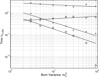
Figure 21.— The theoretical pulse width and the rms centroid variation for each simulation normalized to the observed pulse width $t_{0obs}$. The ratio $t_{0}/t_{0obs}$ is marked with square boxes. The diffractive, refractive, and dispersive contributions to the centroid variation are marked with ‘x’, ’+’ and open circles respectively. The solid lines are empirical models with no theoretical justification.

Estimates of the pulse arrival time are made by integrating over the duration of an observation $T_{obs}$ (typically an hour for a PPTA observation), and also over the observational bandwidth $B$ (typically 256 MHz for a 20 cm PPTA observation). The diffractive intensity fluctuations typically have a $\tau_{\text{dif}}<1$ h, and a $\delta\nu<256$ MHz. So one would expect some smoothing of the diffractive TOA fluctuations. Accordingly we have estimated the diffractive TOA variance with various bandwidths and we find that the rms diffractive TOA variation scales as $(\delta\nu/B)^{1/2}$ as expected. We also find that the rms diffractive TOA variation scales as $(\tau_{\text{dif}}/T_{obs})^{1/2}$. So in reporting the results of the simulations we scale the diffractive TOA variations to $B=\delta\nu$ and $T_{obs}=\tau_{\text{dif}}$. These values can then be scaled using the actual observing time and bandwidth. The resulting values of $T_{\text{dif}}/\tau_{0obs}$ are shown on Figure 21 as ‘x’ symbols. They are fit quite well with an empirical model $T_{\text{dif}}=3.0t_{0obs}(m_{b}^{2})^{-0.087}$.

The refractive time scale is generally much greater than the observing time, and the refractive fluctuations are correlated over the entire frequency band. Thus there is no significant smoothing of the refraction-induced TOA variations. Similarly the dispersive component of the TOA variations is not smoothed by the observational parameters. These components $T_{\text{ref}}$ and $T_{\text{dis}}$ are shown on Figure 21 with ‘+’ symbols and circles respectively. We do not have any theoretical basis for these parameters, but we expect them to be of the order of the pulse width because the pulse broadening is due to the superposition of these centroid variations. We extract empirical models from these data for $T_{\text{ref}}=1.62t_{0obs}(m_{b}^{2})^{-0.62}$; and $T_{\text{dis}}=0.87t_{0obs}(m_{b}^{2})^{-0.66}$. These curves are plotted over the simulated points as solid lines. The dispersive simulation for $m_{b}^{2}$ = 100 seems to be out of character with the rest of the data. This is probably because the simulated screen was not long enough to separate the refractive and dispersive components cleanly. As this screen was already 1 GB in size, we couldn’t increase it easily.

9. Comparison with PPTA Observations

We have used the observed diffractive scintillation parameters of the pulsars in the PPTA to estimate the TOA fluctuations due to scattering. For all the pulsars measurements of $\tau_{\text{dif}}$ and $\delta\nu$ are available at some frequency $f_{obs}$, although they are sometimes quite noisy and apparently variable. These parameters are seldom measured at 1400 MHz, which is the primary frequency at which TOAs are measured with the PPTA, so we scale them all to 1400 MHz first. We use the Kolmogorov scaling for $\tau_{\text{dif}}\propto\text{f}^{1.2}$, but we scale $\delta\nu\propto\text{f}^{4.0}$ as discussed in the previous section. From these we can calculate $m_{b}^{2}=0.773(\text{f}/\delta\nu)^{5/6}$ and $t_{0obs}=1/2\pi\delta\nu$. We then find $T_{\text{dif}}$, $T_{\text{ref}}$, and $T_{\text{dis}}$ at 1400 MHz using the empirical models discussed in the previous section. Finally we use $\tau_{\text{dif}}$ and $\delta\nu$ to estimate the number of independent diffractive scintles in the observation NS = ($T_{\text{obs}}/\tau_{\text{dif}}$)(B/$\delta\nu$). The diffractive contribution to the observed TOA is $T_{\text{dc}}=T_{\text{dif}}/\sqrt{NS}$. The total predicted rms of the TOA is obtained by adding the three components in quadrature. The results are shown in Table 2.

Table 2Predicted centroid variation for PPTA pulsars. The columns to the left of the vertical line are the observations on which the predicted centroid variations to the right of the line are based. The values of $\delta\nu$ and $\tau_{\text{dif}}$ used are the geometric mean of the observation range. The predicted variation has been calculated at 1400 MHz for the first 20 rows, and at 685 MHz for the last row.

source	$f_{obs}$	$\delta\nu$	$\tau_{\text{dif}}$	$m_{b}^{2}$	$t_{0obs}$	$T_{dc}$	$T_{ref}$	$T_{dis}$	$T_{rms}$
	MHz	MHz	min		ns	ns	ns	ns	ns
J0437-4715	660	17.0	7.80	1.94	0.46	0.74	0.46	0.23	0.90
J0613-0200	1369	1.74	23.2	188	83.5	5.60	4.88	2.01	7.69
J0711-6830	685	2.32	25.9	11.7	3.93	2.95	1.28	0.59	3.27
J0711-6830	1369	48.1	67.6	11.8	3.03	2.75	0.98	0.45	2.96
J1022+1001	685	16.0	98.7	2.34	0.57	2.79	0.51	0.25	2.84
J1024-0719	685	15.0	45.2	2.46	0.61	1.93	0.52	0.25	2.02
J1045-4509	3100	3.10	5.14	2324	1234	4.25	15.1	5.63	16.7
J1600-3053	3100	3.62	9.59	2041	1056	5.47	14.0	5.25	16.0
J1603-7202	685	1.68	15.2	15.3	5.44	2.55	1.50	0.68	3.04
J1603-7202	1369	5.69	17.5	70.0	25.6	3.12	2.75	1.18	4.32
J1643-1224	3100	1.33	5.59	4691	2867	6.07	22.8	8.23	25.0
J1713+0747	685	4.45	30.7	6.78	2.05	2.51	0.94	0.44	2.72
J1730-2304	685	2.55	16.1	10.8	3.58	2.25	1.23	0.57	2.62
J1730-2304	1369	11.2	30.3	39.9	13.0	3.18	1.99	0.87	3.85
J1732-5049	1369	3.34	26.5	109.	43.6	4.68	3.56	1.50	6.07
J1744-1144	685	12.8	46.9	2.81	0.71	2.09	0.56	0.27	2.18
J1824-2452	3100	0.81	3.23	7093	4709	5.57	28.9	10.3	31.2
J1857+0943	685	4.42	16.9	6.83	2.07	1.87	0.94	0.44	2.14
J1857+0943	1369	8.22	33.0	51.5	17.7	3.73	2.31	1.00	4.50
J1909-3744	685	7.48	33.2	4.40	1.22	2.15	0.73	0.35	2.30
J1939+2134	1369	2.20	6.40	154.	66.0	2.69	4.36	1.80	5.43
J2124-3358	436	6.90	44.0	0.90	0.22	1.74	0.35	0.18	1.78
J2129-5718	685	2.77	21.6	10.1	3.30	2.52	1.18	0.55	2.84
J2129-5718	1369	76.5	52.6	8.03	1.90	2.04	0.78	0.37	2.21
J2145-0750	685	11.3	47.1	3.12	0.81	2.19	0.60	0.29	2.29
J0437-4715	660	17.0	7.80	14.7	8.07	2.98	2.29	1.04	2.62

The predicted scattering noise at 1400 MHz is less than 50 ns rms for all of the pulsars in the regular PPTA observations. If this prediction is accurate then scattering is not a significant source of timing noise at the PPTA. However we know of two observations of timing noise which is correlated with intensity variations. The first we have already discussed, the timing noise in J0437$-$4715 at 685 MHz is correlated at the diffractive time scale. The observed rms is 1000 ns and the predicted rms is only 2.6 ns. In this case the expected pulse width is only 8.07 ns, so it is difficult to understand how scintillation could cause an rms 100 times larger than the pulse width. The second case of such correlation has been observed in the pulsar J1939$+$2134 at the refractive time scale at 1.4 GHz (Lestrade et al 1998). Here the rms TOA residuals were of the order of 300 ns and the autocorrelation was of the order of 25% at the first time lag. This is consistent with about 150 ns of timing noise correlated with flux. However we only predict 5.4 ns of timing noise, which would not have been observable. The predicted pulse width is only 66 ns, so it is surprising to see such a large observed variation. In these observations the diffractive scale could not be observed, so the correlated rms could be even higher.

The simulations reported here are for a thin scattering layer of homogeneous isotropic turbulence with a Kolmogorov spectrum. The two pulsars in question are well approximated by a thin layer of Kolmogorov turbulence (Ramachandran et al. 2006; You et al. 2007), but the turbulence may not be isotropic or homogeneous. Indeed it has been suggested that J1939$+$2134 underwent an extreme scattering event (Cognard et al. 1993; Lestrade et al. 1998). It is becoming more evident that many pulsars show the effects of anisotropic scattering and it has been shown that anisotropy can have a pronounced effect on pulse broadening (Rickett et al. 2009), but we do not have an estimate of the anisotropy of the scattering for either J0437$-$4715 or J1939$+$2134. It has recently been shown that the scattering in a different pulsar B0834$+$06 is caused by highly inhomogeneous turbulence (Brisken et al. 2009) and this may also be implied by the earlier observations of Hill et al. (2005). It is easy to imagine that inhomogeneous turbulence would greatly enhance refractive scattering but it is much less obvious what it might do to diffractive effects. The simulation can be extended to study the effects of anisotropy and inhomogeneity and we are undertaking such an extension.

It is also possible that there is an unrecognized mechanism which causes timing fluctuations which are correlated with signal to noise ratio. If so, it should be correctable in the same way, but it is very important to understand the mechanism.

10. Conclusions

Simulations have been shown to be a very useful tool in understanding observations of scattering in the interstellar plasma. The simulation engine has been regularized to the point where it can be used by others and it is available from the authors. Here we show a number of examples where simulations have allowed us to understand long standing peculiarities in the observations. We also show that the simulated timing noise due to homogeneous isotropic turbulence is considerably smaller than two cases of observed timing noise which is correlated with intensity fluctuations. This opens a number of interesting questions about the effects of the assumptions of homogeneous isotropic turbulence, and about the observations themselves.

References

- Blandford & Narayan (1985) Blandford, R.D. and Narayan, R. 1985, MNRAS213, 591.
- Bhat et al. (1999) Bhat, N.D.R., Rao, A.P. & Gupta, Y. 1999, ApJS, 121, 483.
- Brisken et al. (2009) Brisken, W., Macquart, J.-P., Gao, J.J., Rickett, B.J., Coles, W.A., Deller, A., and Tingay, S. 2009, ApJ, accepted, arXiv:0910.5654 [astro-ph].
- Codona et al. (1986) Codona, J. L., Creamer, D. B., Flatte, S. M., Frehlich, R. G., & Henyey, F. S. 1986, Radio Sci., 21, 805.
- Cognard et al. (1993) Cognard,I., Bourgois, G., Lestrade, J.F.,Biraud, F., Aubry, D. Darchy, B., Drouhin, J.P. 1993, Nature, 336, 320.
- Coles & Filice (1984) Coles, W. A., and Filice, J.P. 1984, Nature 312, 251.
- Coles et al. (1987) Coles, Wm. A., Frehlich, R. G., Rickett, B.J. & Codona, J.L. 1987, ApJ, 315, 666.
- (8) Coles, Wm. A., Filice, J. P., Frehlich, R. G., & Yadlowsky, M. 1995, Appl. Opt., 34, 2089.
- (9) Coles, W. A.; Grall, R. R.; Klinglesmith, M. T.; Bourgois, Gabriel, 1995, JGR, 17069
- Cordes (1986) Cordes, J. M. 1986, ApJ, 311, 183
- Cordes, Pidwerbetsky, & Lovelace (1986) Cordes, J. M., Pidwerbetsky, A., & Lovelace, R. V. E. 1986, ApJ, 310, 737
- Cordes (1990) Cordes J. M., Wolszczan, A., Dewey, R. J., Blaskiewisicz, M., Stinebring, D.R., 1990, ApJ, 349, 245.
- Cordes & Rickett (1998) Cordes, J. M. & Rickett, B. J. 1998, ApJ, 507, 846
- Cordes et al. (2006) Cordes, J. M., Rickett, B. J., Stinebring, D. R. & Coles, W. A. 2006, ApJ, 637, 346-365.
- Ewing (1970) Ewing, M. S., Batchelor, R. A., Friefeld, R. D., Price, R. M., Staelin, D. H. 1970. Ap. J. 162 : L169-172.
- Fiedler et al. (1987) Fiedler, R. L., Dennison, B., Johnston, K. J., & Hewish, A. 1987, Nature, 326, 675
- Foster and Cordes (1990) Foster, R. S. and Cordes, J. M. 1990, ApJ, 364,123.
- Gochelashvily and Shishov (1971) Gochelashvily, K.A. and Shishov, V.I. 1971, Optical Acta, 18, 313.
- Goodman and Narayan (2006) Goodman, J. and Narayan, R. 2006, ApJ, 636, 510-527.
- Gupta et al. (1994) Gupta, Y., Rickett, B.J., and Lyne, A.G. 1994, MNRAS, 269, 1035.
- Hamidouche and Lestrade (2007) Hamidouche, M. and Lestrade, J.-F. 2007, A&A, 468, 193
- Hankins et al. (2003) Hankins, T. H., Kern, J. S., Weatherall J. C. & Eilek, J.A. 2003, Nature, 422, 141
- Hewish (1980) Hewish, A. 1980, MNRAS, 192, 799.
- Hewish et al. (1985) Hewish, A.; Wolszczan, A.; Graham, D. A. 1985, MNRAS, 213, 167.
- Hill et al. (2005) Hill, A.S., Stinebring, D.R., Asplund, C.T., Berwick, D.E., Everett, W.B., & Hinkel, N.R. 2005, ApJ, 619, L171-174.
- Lestrade et al. (1998) Lestrade, J.-F., Rickett, B. J., & Cognard, I. 1998, A&A334, 1068.
- Narayan (1992) Narayan, R. 1992, Phil. Trans. R. Soc. London A, 341, 151
- Prokhorov et al. (1975) Prokhorov, A.M., Bunkin, F.V., Gochelashvily, K.S., and Shishov, V.I. 1975, Proc.I.E.E.E., 63, 790.
- Ramachandran et al. (2006) Ramachandran, R., Demorest, P., Backer, D.C., Cognard, I., and Lommen, A. 2006, ApJ, 645, 303.
- Rankin et al. (1970) Rankin, J. M.; Comella, J. M.; Craft, H. D., Jr.; Richards, D. W.; Campbell, D. B.; Counselman, C. C., III, 1970, ApJ, 162, 707
- Rawley et al. (1988) Rawley, L. A.; Taylor, J. H.; Davis, M. M., 1988, ApJ, 326, 947
- Rickett (1969) Rickett, B.J., 1969, Nature, 221, 158
- Rickett et al. (1987) Rickett, B.J., Coles, W. A., and Bourgois, G. 1984, A&A, 134, 390.
- Rickett,Coles & Markkanen, (2000) Rickett, B. J.; Coles, Wm. A.; Markkanen, J., 2000, ApJ, 533, 304
- Rickett et al. (2009) Rickett, B. J., Johnston, S., Tomlinson, T., and Reynolds, J. 2009, MNRAS. 395, 1391-1402.
- Rickett (1990) Rickett, B. J. 1990, ARA&A, 28, 561
- Roberts and Ables (1982) Roberts, J. A., Ables, J. G. 1982. MNRAS. 201 : 1119-1138.
- Shishov (1974) Shishov, V. I. 1974. Soviet Astron. 17 : 598-602.
- Stinebring et al. (2001) Stinebring, D. R., McLaughlin, M. A., Cordes, J. M., Becker, K. M., Goodman, J. E. E., Kramer, M. A., Sheckard, J. L., & Smith, C. T. 2001, ApJ, 549, L97.
- Tatarskii, (1967) Tatarski, V.I. 1967, “Propagation of waves in a turbulent atmosphere”, Moscow, Nauka, in Russian.
- Verbiest et al. (2008) Verbiest, J.P.W., Bailes, M., van Straten, W., Hobbs, G.B., Edwards, R.T., Manchester, R.N., Bhat, N.D.R., Sarkissian, J.M., Jacoby, B.A. and Kulkarni, S.R. 2008, ApJ, 679, 675-680.
- Verbiest et al. (2009) Verbiest, J. P. W., Bailes, M., Coles, W. A., Hobbs, G. B., van Straten, W., Champion, D. J., Jenet, F. A., Manchester, R. N., Bhat, N. D. R., Sarkissian, J. M., Yardley, D., Burke-Spolaor, S., Hotan, A. W. and You, X. P., 2009, MNRAS, 400, 951.
- You et al. (2007) You, XP; Hobbs, G.; Coles, WA; Manchester, RN; Edwards, R.; Bailes, M.; Sarkissian, J.; Verbiest, JPW; van Straten, W.; Hotan, A.; Ord, S.; Jenet, F.; Bhat, NDR; Teoh, A. 2007, MNRAS, 378, 493.