Madelung Representation and Exactly Solvable Schrödinger-Burgers Equations with Variable Parameters

Abstract

We construct a Madelung fluid model with specific time variable parameters as dissipative quantum fluid and linearize it in terms of Schrödinger equation with time dependent parameters. It allows us to find exact solutions of the nonlinear Madelung system in terms of solutions of the Schrödinger equation and the corresponding classical linear ODE with variable frequency and damping. For the complex velocity field the Madelung system takes the form of a nonlinear complex Schrödinger-Burgers equation, for which we obtain exact solutions using complex Cole-Hopf transformation. In particular, we discuss and give exact results for nonlinear Madelung systems related with Caldirola-Kanai type dissipative harmonic oscillator.

1 Introduction

In the recent years the Madelung fluid description of quantum mechanics has been applied to some fields where the quantum formalism is a useful tool for describing the evolution of classical (quantum-like) systems and studying the dispersionless or semiclassical limit of nonlinear partial differential equations of Schrödinger type, [1]. The Madelung fluid representation, proposed first by [2], being a complex quantity, represents a solution of the Schrödinger equation, in terms of modulus and phase. Substituted to the Schrödinger equation it allows to obtain a pair of nonlinear hydrodynamic type equations. Thus, the Madelung fluid equations are nonlinear system of PDEs, while the Schrödinger equation is the linear one. Then, the Madelung transform is a complex linearization transform, similar to the Cole-Hopf transformation, linearizing the nonlinear Burgers equation in terms of the linear heat equation, see [4] and [5]. Nonlinear models admitting such type of direct linearization are called by F. Calogero as C-integrable models.

In this work, we construct a Madelung fluid model with time variable parameters as dissipative quantum fluid and linearize it in terms of Schrödinger equation with time dependent parameters. It allows us to find exact solution of the nonlinear Madelung system in terms of solutions to the Schrödinger equation and the corresponding classical linear ODE with variable frequency and damping. Moreover, the Madelung system written for the complex velocity field takes the form of a nonlinear complex Schrödinger-Burgers equation, which exact solutions we obtain using complex Cole-Hopf transformation. As known, in the usual Cole-Hopf transformation zeros of the linear heat equation lead to poles in the corresponding Burgers equation. Similarly, in our case, by the complex Cole-Hopf transformation zeros of the Schrödinger equation transform to pole singularities in the complex Schrödinger-Burgers equation. Thus, using exact solutions of the linear problem, one can find also the dynamics of the poles in the corresponding nonlinear problem. As an exactly solvable model, we describe a dissipative nonlinear complex Schrödinger-Burgers equation of Caldirola-Kanai type, [11], [12]. Exact solutions of the nonlinear models are found and the motion of zeros and poles is discussed explicitly. Some illustrative plots are constructed.

2 The Schrödinger Equation and its Madelung Representation

2.1 Solution of the Schrödinger Equation

Consider the one-dimensional Schrödinger equation for harmonic oscillator with time-dependent parameters

$$i\hbar\frac{\partial\Psi}{\partial t}=-\frac{\hbar^{2}}{2\mu(t)}\frac{\partial^{2}\Psi}{\partial q^{2}}+\frac{\mu(t)\omega^{2}(t)}{2}q^{2}\Psi,$$ (1)

and initial condition

$$\Psi(q,t_{0})=\psi(q),\,\,\,\,\,\,-\infty<q<\infty.$$ (2)

Using the Evolution operator method, [8], it was proved that, see [7], if $x(t)$ is the solution of the classical equation of motion

$$\ddot{x}+\frac{\dot{\mu}(t)}{\mu(t)}\dot{x}+\omega^{2}(t)x=0,\,\,\,x(t_{0})=x_{0}\neq 0,\,\,\,\dot{x}(t_{0})=0,$$ (3)

then the solution of the IVP (1)-(2) is found as $\Psi(q,t)=\widehat{U}(t,t_{0})\psi(q),$ where the evolution operator is

$$\widehat{U}=\exp\left(\frac{i}{2}fq^{2}\right)\,\exp\left(h(q\frac{\partial}{\partial q}+\frac{1}{2})\right)\,\exp\left(-\frac{i}{2}g\frac{\partial^{2}}{\partial q^{2}}\right)$$

and the auxiliary functions are

$$f(t)=\frac{\mu(t)}{\hbar}\frac{\dot{x}(t)}{x(t)};\,\,\,g(t)=-\hbar x^{2}(t_{0})\int^{t}\frac{d\xi}{\mu(\xi)x^{2}(\xi)},\,\,\,\,g(t_{0})=0;\,\,\,h(t)=\ln\frac{|x(t_{0})|}{|x(t)|}.$$

In particular, if the initial function is the normalized eigenstate corresponding to eignenvalue $E_{k}=\hbar^{2}\Omega_{0}(k+1/2)$ of the Hamiltonian for the standard harmonic oscillator, that is

$$\varphi_{k}(q)=N_{k}e^{-\frac{\Omega_{0}}{2}q^{2}}H_{k}(\sqrt{\Omega_{0}}q),\,\,\,\,\,k=0,1,2,...,$$ (4)

then, the time-evolved state for the Schrödinger equation (1) is

$$\Psi_{k}(q,t) = \hat{U}(t,t_{0})\varphi_{k}(q)$$ (5)

$$= N_{k}\sqrt{R(t)}\times\exp\left(i\left(k+\frac{1}{2}\right)\arctan(\Omega_{0}g(t))\right)$$

$$\times\exp\left(i\left(\frac{\mu(t)\dot{x}(t)}{2\hbar x(t)}-\frac{\Omega_{0}^{2}}{2}g(t)R^{2}(t)\right)q^{2}\right)$$

$$\times\exp\left(-\frac{\Omega_{0}}{2}R^{2}(t)q^{2}\right)\times H_{k}\left(\sqrt{\Omega_{0}}R(t)q\right).$$

where

$$R(t)=\left(\frac{x_{0}^{2}}{x^{2}(t)+(\Omega_{0}x(t)g(t))^{2}}\right)^{\frac{1}{2}}.$$ (6)

The corresponding probability density is then

$$\rho_{k}(q,t)=\frac{1}{2^{k}k!\sqrt{\pi}}\times\sqrt{\Omega_{0}}R(t)\times\exp\left(-\left(\sqrt{\Omega_{0}}R(t)q\right)^{2}\right)\times H_{k}^{2}\left(\sqrt{\Omega_{0}}R(t)q\right).$$

2.2 Madelung representation

As known, Madelung representation of the complex-valued wave function

$$\Psi(q,t)=\sqrt{\rho}\exp\left(\frac{i}{\hbar}S\right)=\exp\left(\frac{1}{2}\ln\rho+\frac{i}{\hbar}S\right),$$ (7)

where $\rho=\rho(q,t)$ is the probability density and $S=S(q,t)$ is the action, both being real-valued functions, decomposes the Schrödinger equation (1) into a system of nonlinear coupled partial differential equations,

$$\frac{\partial S}{\partial t}+\frac{1}{2\mu(t)}\left(\frac{\partial S}{\partial q}\right)^{2}+\frac{\mu(t)\omega^{2}(t)}{2}q^{2}=\frac{\hbar^{2}}{2\mu(t)}\left[\frac{1}{\sqrt{\rho}}\frac{\partial^{2}\sqrt{\rho}}{\partial q^{2}}\right]$$

$$\frac{\partial\rho}{\partial t}+\frac{\partial}{\partial q}\left[\rho\frac{1}{\mu(t)}\frac{\partial S}{\partial q}\right]=0.$$ (8)

The first equation may be viewed as a generalization of the usual Hamilton-Jacobi equation. The term with explicit $\hbar$ dependence is the quantum potential encoding the quantum aspects of the theory. When $\hbar\rightarrow 0,$ the equation becomes Hamilton-Jacobi equation for a non-relativistic particle with time dependent mass. The second equation is a continuity equation expressing the conservation of probability density. Using the relation (7), one can see that the system (8), with general initial conditions

$$S(q,t_{0})=\tilde{S}(q),\,\,\rho(q,t_{0})=\tilde{\rho}(q),$$ (9)

$\tilde{S}(q),\tilde{\rho}(q)$ being real-valued functions, has formal solution

$$S(q,t)=-i\hbar\ln\left(\frac{\Psi(q,t)}{|\Psi(q,t)|}\right),\,\,\rho(q,t)=|\Psi(q,t)|^{2},$$ (10)

where $\Psi(q,t)$ is a solution of the Schrödinger equation (1) with initial condition

$$\Psi(q,t_{0})=\sqrt{\tilde{\rho}(q)}\exp(\frac{i}{\hbar}\tilde{S}(q)).$$ (11)

We remark that, since $\Psi(q,t)$ is complex-valued, in general $S(q,t)$ is multi-valued, i.e. $S(q,t)=-i\hbar\ln(\Psi/|\Psi|)+2\pi n\hbar,$ $n=0,\pm 1,\pm 2,...,$ but fixing the initial condition $S(q,t_{0})=\tilde{S}(q)$ leads to a single-valued solution of the IVP.

2.3 Madelung Hydrodynamic Equations

Introducing classical velocity, $v(q,t)=\displaystyle\frac{1}{\mu(t)}\frac{\partial S}{\partial q}\,,$ the system (8) transforms to Madelung fluid equations

$$\left\{\begin{array}[]{ll}\displaystyle\frac{\partial v}{\partial t}+\frac{\dot{\mu}(t)}{\mu(t)}v+v\frac{\partial v}{\partial q}=-\frac{1}{\mu(t)}\frac{\partial}{\partial q}\left[\frac{-\hbar^{2}}{2\mu(t)}\left(\frac{1}{\sqrt{\rho}}\frac{\partial^{2}\sqrt{\rho}}{\partial q^{2}}\right)+\frac{\mu(t)\omega^{2}(t)}{2}q^{2}\right],\\ \displaystyle\frac{\partial\rho}{\partial t}+\frac{\partial}{\partial q}\left[\rho v\right]=0.\end{array}\right.$$ (14)

These equations are similar to the classical hydrodynamic equations where $\rho(q,t)$ is the density and $v(q,t)$ is the velocity field of the one-dimensional fluid. The system of fluid equations (14) with general initial conditions

$$v(q,t_{0})=\tilde{v}(q),\,\,\,\rho(q,t_{0})=\tilde{\rho}(q),$$

$\tilde{v}(q)$,$\,\tilde{\rho}(q)$ being real-valued functions, has formal solution

$$v(q,t)=-\frac{i\hbar}{\mu(t)}\frac{\partial}{\partial q}\ln\left(\frac{\Psi(q,t)}{|\Psi(q,t)|}\right),\,\,\rho(q,t)=|\Psi(q,t)|^{2},$$ (15)

where $\Psi(q,t)$ is solution of the Schrödinger equation (1) subject to the initial condition

$$\Psi(q,t_{0})=\sqrt{\tilde{\rho}(q)}\exp\left(\frac{i}{\hbar}\mu(t_{0})\int^{q}\tilde{v}(\xi)d\xi\right).$$

3 Potential Schrödinger-Burgers Equation

Writing the wave function in the form

$$\Psi(q,t)=\exp\left(\frac{i}{\hbar}\mu(t)F(q,t)\right),$$

where $F(q,t)$ is a complex potential, the IVP for the Schrödinger equation (1) transforms to the following IVP for the nonlinear potential Schrödinger-Burgers equation

$$\left\{\begin{array}[]{ll}\displaystyle\frac{\partial F}{\partial t}+\frac{\dot{\mu}(t)}{\mu(t)}F+\frac{1}{2}(\frac{\partial F}{\partial q})^{2}+\frac{\omega^{2}(t)}{2}q^{2}=\frac{i\hbar}{2\mu(t)}\frac{\partial^{2}F}{\partial q^{2}}\,\,,\\ F(q,t_{0})=\widetilde{F}(q),\end{array}\right.$$ (18)

Therefore, the formal solution of this problem is

$$F(q,t)=-\frac{i\hbar}{\mu(t)}(\ln\Psi(q,t))\,\,,$$ (19)

where $\Psi(q,t)$ is solution of the Schrödinger equation (1), with initial condition

$$\Psi(q,t_{0})=\exp\left(\frac{i}{\hbar}\mu(t_{0})\widetilde{F}(q)\right).$$

Note again, that fixing the initial condition we obtain a single-valued solution $F(q,t).$ Now, using the Madelung representation (7) and relation (19), one can write

$$F(q,t)=\textsf{F}_{1}+i\textsf{F}_{2}=\frac{1}{\mu(t)}S-\frac{i\hbar}{2\mu(t)}\ln\rho,$$ (20)

where $\textsf{F}_{1}=\textsf{F}_{1}(q,t)$ represents the velocity potential, and $\textsf{F}_{2}=\textsf{F}_{2}(q,t)$ the stream function of the fluid, ( $\textsf{F}_{1},\textsf{F}_{2}$ being real-valued). Accordingly, the real and imaginary parts of the potential Schrödinger-Burgers equation (18) become

$$\left\{\begin{array}[]{ll}\displaystyle\frac{\partial\textsf{F}_{1}}{\partial t}+\frac{\dot{\mu}}{\mu}\textsf{F}_{1}+\frac{1}{2}\left((\frac{\partial\textsf{F}_{1}}{\partial q})^{2}-(\frac{\partial\textsf{F}_{2}}{\partial q})^{2}\right)+\frac{\omega^{2}(t)}{2}q^{2}=-\frac{\hbar}{2\mu}\frac{\partial^{2}\textsf{F}_{2}}{\partial q^{2}},\\ \displaystyle\frac{\partial\textsf{F}_{2}}{\partial t}+\frac{\dot{\mu}}{\mu}\textsf{F}_{2}+\frac{\partial\textsf{F}_{1}}{\partial q}\frac{\partial\textsf{F}_{2}}{\partial q}=\frac{\hbar}{2\mu}\frac{\partial^{2}\textsf{F}_{1}}{\partial q^{2}}.\end{array}\right.$$ (23)

Using the relations (20) and (10), one can see that the nonlinear system (23) with general initial conditions

$$\textsf{F}_{1}(q,t_{0})=\widetilde{\textsf{F}}_{1}(q),\,\textsf{F}_{2}(q,t_{0})=\widetilde{\textsf{F}}_{2}(q)$$

and $\widetilde{\textsf{F}}_{1}(q)$, $\widetilde{\textsf{F}}_{2}(q)$ real-valued functions, has solution of the form

$$\textsf{F}_{1}=-\frac{i\hbar}{\mu(t)}\ln\left(\frac{\Psi}{|\Psi|}\right),\,\textsf{F}_{2}=-\frac{\hbar}{\mu(t)}\ln(|\Psi|),$$

where $\Psi(q,t)$ is solution of the Schrödinger equation (1) with initial condition

$$\Psi(q,t_{0})=\exp\left(\frac{i}{\hbar}\mu(t_{0})\widetilde{\textsf{F}}_{1}(q)\right)\times\exp\left(-\frac{1}{\hbar}\mu(t_{0})\widetilde{\textsf{F}}_{2}(q)\right).$$

4 Schrödinger-Burgers Equation

Representation of the wave function in the form

$$\Psi(q,t)=\exp\left(\frac{i}{h}\mu(t)\int^{q}V(\xi,t)d\xi\right),$$ (24)

where $V(q,t)$ is a complex velocity, transforms the IVP for the Schrödinger equation (1) to the following IVP for a nonlinear Schrödinger-Burgers equation with time dependent coefficients

$$\left\{\begin{array}[]{ll}\displaystyle\frac{\partial V}{\partial t}+\frac{\dot{\mu}(t)}{\mu(t)}V+V\frac{\partial V}{\partial q}+\omega^{2}(t)q=\frac{i\hbar}{2\mu(t)}\frac{\partial^{2}V}{\partial q^{2}}\,\,,\\ V(q,t_{0})=\widetilde{V}(q)\,\,,\end{array}\right.$$ (27)

Solution of this IVP is found by the complex Cole-Hopf transformation

$$V(q,t)=-\frac{i\hbar}{\mu(t)}\frac{\partial}{\partial q}(\ln\Psi(q,t)),$$ (28)

where $\Psi(q,t)$ is solution of the the Schrödinger equation (1), corresponding to initial condition

$$\Psi(q,t_{0})=\psi(q)=\exp\left(\frac{i}{\hbar}\mu(t_{0})\int^{q}\widetilde{V}(\xi)d\xi\right).$$

Using the Madelung representation (7) and the complex Cole-Hopf transformation (28) one can write the complex velocity function in the form

$$V(q,t)=v+iu=\frac{1}{\mu(t)}\frac{\partial S}{\partial q}-\frac{i\hbar}{2\mu(t)}\frac{\partial}{\partial q}(\ln\rho),$$ (29)

where $v=v(q,t),$ $\,u=u(q,t)$ are real-valued, $v$ represents the classical velocity, and $u$ the quantum velocity. This splits the Schrödinger-Burgers equation into real and imaginary parts, respectively,

$$\left\{\begin{array}[]{ll}\displaystyle\frac{\partial v}{\partial t}+\frac{\dot{\mu}(t)}{\mu(t)}v+v\frac{\partial v}{\partial q}+\omega^{2}(t)q=\frac{-\hbar}{2\mu(t)}\frac{\partial^{2}u}{\partial q^{2}}+u\frac{\partial u}{\partial q},\\ \displaystyle\frac{\partial u}{\partial t}+\frac{\dot{\mu}(t)}{\mu(t)}u+u\frac{\partial v}{\partial q}+v\frac{\partial u}{\partial q}=\frac{\hbar}{2\mu(t)}\frac{\partial^{2}v}{\partial q^{2}}.\end{array}\right.$$ (32)

The first equation is a hydrodynamic equation for the classical velocity, and the second one is the transport equation for the quantum velocity. Using relations (29) and (10), we find that the system of nonlinear coupled equations (32) with general initial conditions

$$v(q,t_{0})=\tilde{v}(q),\,\,u(q,t_{0})=\tilde{u}(q)$$

has formal solution

$$v=-\frac{i\hbar}{\mu(t)}\frac{\partial}{\partial q}\ln\left(\frac{\Psi}{|\Psi|}\right),\,\,u=-\frac{\hbar}{\mu(t)}\frac{\partial}{\partial q}\ln(|\Psi|),$$

where $\Psi=\Psi(q,t)$ is a solution of the Schrödinger equation (1) with general initial condition

$$\Psi(q,t_{0})=\exp(\frac{i\mu(t_{0})}{\hbar}\int^{q}\tilde{v}(\xi)d\xi)\times\exp(-\frac{\mu(t_{0})}{\hbar}\int^{q}\tilde{u}(\xi)d\xi).$$

5 Exactly Solvable Nonlinear Models

The Caldirola-Kanai model, [11],[12], which is a one dimensional system with an exponentially increasing mass, is the best known model of harmonic oscillator with time-dependent parameters. Here, using the general discussion in the previous parts, we obtain exact solutions of the nonlinear problems related with the Caldirola-Kanai oscillator

$$\left\{\begin{array}[]{ll}\displaystyle i\hbar\frac{\partial\Psi}{\partial t}=-\frac{\hbar^{2}}{2}e^{-\gamma t}\frac{\partial^{2}\Psi}{\partial q^{2}}+\frac{1}{2}\omega_{0}^{2}e^{\gamma t}q^{2}\Psi,\\ \displaystyle\Psi(q,0)=\psi(q),\,\,\,\,\,q\in R,\end{array}\right.$$ (35)

where $\mu(t)=e^{\gamma t}$ is the integrating factor, $\Gamma(t)=\gamma$ is the damping term, $\gamma>0$, and $\omega^{2}(t)=\omega_{0}^{2}$ is a constant frequency. As known, solutions of the Cadirola-Kanai oscillator can be found in terms of the solution to the corresponding classical equation of motion

$$\ddot{x}+\gamma\dot{x}+\omega_{0}^{2}x=0,\,\,\,\,\,x(0)=x_{0}\neq 0,\,\,\,\dot{x}(0)=0.$$ (36)

Clearly, according to the sign of $\Omega^{2}=\omega_{0}^{2}-(\gamma^{2}/4)$ there are three different type of behavior- critical damping, under damping and over damping. In this article, we discuss the critical damping case, i.e. $\Omega^{2}=0.$ If $\Omega^{2}=\omega_{0}^{2}-(\gamma^{2}/4)=0$, then the classical equation (36) has solution

$$x(t)=x_{0}e^{-\frac{\gamma t}{2}}(1+\frac{\gamma}{2}t),$$

and it follows that

$$g(t)=\frac{-\hbar t}{1+\frac{\gamma}{2}t},\,\,\,\,\,\,\,\,\,\,R(t)=\left(\frac{e^{\gamma t}}{(1+\frac{\gamma}{2}t)^{2}+w_{0}^{2}t^{2}}\right)^{1/2}.$$

Then, using (5), exact solutions of the Schrödinger equation (35) with initial conditions $\Psi(q,0)=\varphi_{k}(q),$ are

$$\Psi_{k}(q,t) = N_{k}\left(\frac{e^{\gamma t}}{(1+\frac{\gamma}{2}t)^{2}+w_{0}^{2}t^{2}}\right)^{1/4}\exp\left(i(k+\frac{1}{2})\arctan(\frac{-\omega_{0}t}{1+\frac{\gamma}{2}t})\right)$$

$$\times\exp\left(-i\frac{\omega_{0}^{2}}{2\hbar}\left(\frac{te^{\gamma t}}{1+\frac{\gamma}{2}t}\right)\left(1-\frac{1}{(1+\frac{\gamma}{2}t)^{2}+w_{0}^{2}t^{2}}\right)q^{2}\right)$$

$$\times\exp\left(-\frac{\omega_{0}}{2\hbar}\left(\frac{e^{\gamma t}}{(1+\frac{\gamma}{2}t)^{2}+w_{0}^{2}t^{2}}\right)q^{2}\right)H_{k}\left(\sqrt{\frac{\omega_{0}}{\hbar}}\left(\frac{e^{\gamma t}}{(1+\frac{\gamma}{2}t)^{2}+w_{0}^{2}t^{2}}\right)^{1/2}q\right).$$

a. Madelung representation of Caldirola-Kanai Oscillator. Madelung representation of the wave function decomposes the Schrödinger equation (35) into a system of nonlinear coupled partial differential equations,

$$\left\{\begin{array}[]{ll}\displaystyle\frac{\partial S}{\partial t}+\frac{1}{2}e^{-\gamma t}\left(\frac{\partial S}{\partial q}\right)^{2}+\frac{\omega_{0}^{2}}{2}e^{\gamma t}q^{2}=\frac{\hbar^{2}}{2}e^{-\gamma t}\left[\frac{1}{\sqrt{\rho}}\frac{\partial^{2}\sqrt{\rho}}{\partial q^{2}}\right],\\ \displaystyle\frac{\partial\rho}{\partial t}+e^{-\gamma t}\frac{\partial}{\partial q}\left[\rho\frac{\partial S}{\partial q}\right]=0.\end{array}\right.$$

This system of equations with specific initial conditions

$$S(q,0)=0,\,\,\rho_{k}(q,0)=N_{k}^{2}\exp\left(-\frac{\omega_{0}}{\hbar}q^{2}\right)H_{k}^{2}\left(\sqrt{\frac{\omega_{0}}{\hbar}}q\right),$$

has exact solutions of the form

$$S_{k}(q,t)=\left(-\frac{\omega_{0}^{2}}{2}\left(\frac{te^{\gamma t}}{1+\frac{\gamma}{2}t}\right)\left(1-\frac{1}{(1+\frac{\gamma}{2}t)^{2}+w_{0}^{2}t^{2}}\right)q^{2}\right)+\left(\hbar(k+\frac{1}{2})\arctan(\frac{-\omega_{0}t}{1+\frac{\gamma}{2}t})\right),$$

$$\rho_{k}(q,t) = N_{k}^{2}\left(\frac{e^{\gamma t}}{(1+\frac{\gamma}{2}t)^{2}+w_{0}^{2}t^{2}}\right)^{1/2}\exp\left(-\frac{\omega_{0}}{\hbar}\left(\frac{e^{\gamma t}}{(1+\frac{\gamma}{2}t)^{2}+w_{0}^{2}t^{2}}\right)q^{2}\right)$$

$$\times H_{k}^{2}\left(\sqrt{\frac{\omega_{0}}{\hbar}}\left(\frac{e^{\gamma t}}{(1+\frac{\gamma}{2}t)^{2}+w_{0}^{2}t^{2}}\right)^{1/2}q\right).$$

b. Hydrodynamic equations. The system of hydrodynamic equations for the velocity and density of the fluid

$$\left\{\begin{array}[]{ll}\displaystyle\frac{\partial v}{\partial t}+\gamma v+v\frac{\partial v}{\partial q}=-e^{-\gamma t}\frac{\partial}{\partial q}\left[\frac{-\hbar^{2}e^{-\gamma t}}{2\sqrt{\rho}}\frac{\partial^{2}\sqrt{\rho}}{\partial q^{2}}+\frac{\omega_{0}^{2}}{2}e^{\gamma t}q^{2}\right]\\ \displaystyle\frac{\partial\rho}{\partial t}+\frac{\partial}{\partial q}\left[\rho v\right]=0,\end{array}\right.$$

with specific initial conditions

$$v(q,0)=0,\,\,\rho_{k}(q,0)=N_{k}^{2}\exp\left(-\frac{\omega_{0}}{\hbar}q^{2}\right)H_{k}^{2}\left(\sqrt{\frac{\omega_{0}}{\hbar}}q\right).$$

has solutions

$$v(q,t)=\left(-\omega_{0}^{2}\left(\frac{t}{1+\frac{\gamma}{2}t}\right)\left(1-\frac{1}{(1+\frac{\gamma}{2}t)^{2}+w_{0}^{2}t^{2}}\right)q\right)$$

and $\rho_{k}(q,t)$ given by (5).

c. The potential Schrödinger-Burgers equation. The IVP for potential Schrödinger-Burgers equation

$$\left\{\begin{array}[]{ll}\displaystyle\frac{\partial F}{\partial t}+\gamma F+\frac{1}{2}(\frac{\partial F}{\partial q})^{2}+\frac{\omega_{0}^{2}}{2}q^{2}=\frac{i\hbar}{2}e^{-\gamma t}(\frac{\partial^{2}F}{\partial q^{2}}),\\ F_{k}(q,0)=i\left(\frac{\omega_{0}}{2}q^{2}-\hbar\ln(N_{k}H_{k}(\sqrt{\frac{\omega_{0}}{\hbar}}q))\right),\,\,\,\,\,\,k=0,1,2,...\end{array}\right.$$ (42)

has solutions $F_{k}(q,t)=\textsf{F}_{1,k}(q,t)+i\textsf{F}_{2,k}(q,t),$ where

$$\textsf{F}_{1,k}=-\frac{\omega_{0}^{2}}{2}\left(\frac{t}{1+\frac{\gamma}{2}t}\right)\left(1-\frac{1}{(1+\frac{\gamma}{2}t)^{2}+w_{0}^{2}t^{2}}\right)q^{2}+\hbar e^{-\gamma t}(k+\frac{1}{2})\arctan(\frac{-\omega_{0}t}{1+\frac{\gamma}{2}}),$$

$$\textsf{F}_{2,k} = \frac{\omega_{0}}{2}\left(\frac{1}{(1+\frac{\gamma}{2}t)^{2}+w_{0}^{2}t^{2}}\right)q^{2}-\hbar e^{-\gamma t}\ln\left[N_{k}\left(\frac{e^{-(\gamma/2)t}}{(1+\frac{\gamma}{2}t)^{2}+w_{0}^{2}t^{2}}\right)^{1/2}\right]$$

$$-\hbar e^{-\gamma t}\ln H_{k}\left(\sqrt{\frac{\omega_{0}}{\hbar}\left(\frac{e^{\gamma t}}{(1+\frac{\gamma}{2}t)^{2}+w_{0}^{2}t^{2}}\right)}\,\,\,q\right).$$

d. The Schrödinger-Burgers equation. The IVP for the non-linear complex Schrödinger-Burgers equation

$$\left\{\begin{array}[]{ll}\displaystyle\frac{\partial V}{\partial t}+\gamma V+V\frac{\partial V}{\partial q}+\omega_{0}^{2}q=i\hbar\frac{e^{-\gamma t}}{2}\frac{\partial^{2}V}{\partial q^{2}},\\ \displaystyle V_{k}(q,0)=i\left[\omega_{0}q-2k\sqrt{\hbar\omega_{0}}\left(\frac{H_{k-1}(\sqrt{\frac{\omega_{0}}{\hbar}}q)}{H_{k}(\sqrt{\frac{\omega_{0}}{\hbar}}q)}\right)\right],\end{array}\right.$$ (45)

has solutions

$$V_{k}(q,t)=\left(-\omega_{0}^{2}\left(\frac{t}{1+\frac{\gamma}{2}t}\right)\left(1-\frac{1}{(1+\frac{\gamma}{2}t)^{2}+w_{0}^{2}t^{2}}\right)q\right)+i\left(\frac{\omega_{0}}{(1+\frac{\gamma}{2}t)^{2}+w_{0}^{2}t^{2}}\right)q$$

$$-i2k\sqrt{\hbar\omega_{0}}e^{-\gamma t}\left(\frac{e^{\gamma t}}{(1+\frac{\gamma}{2}t)^{2}+w_{0}^{2}t^{2}}\right)^{1/2}\times\left(\frac{H_{k-1}(\sqrt{\frac{\omega_{0}}{\hbar}\left(\frac{e^{\gamma t}}{(1+\frac{\gamma}{2}t)^{2}+w_{0}^{2}t^{2}}\right)}\,\,\,q)}{H_{k}(\sqrt{\frac{\omega_{0}}{\hbar}\left(\frac{e^{\gamma t}}{(1+\frac{\gamma}{2}t)^{2}+w_{0}^{2}t^{2}}\right)}\,\,\,q)}\right).$$ (46)

The complex velocity function, written in the form $V(q,t)=v(q,t)+iu(q,t),$ where $v,u$ are real-valued functions, splits the Schrödinger-Burgers equation (45) into the system

$$\left\{\begin{array}[]{ll}\displaystyle\frac{\partial v}{\partial t}+\gamma v+v\frac{\partial v}{\partial q}-u\frac{\partial u}{\partial q}+\omega^{2}_{0}q=-\frac{\hbar}{2}e^{-\gamma t}\frac{\partial^{2}u}{\partial q^{2}}\,\,,\\ \displaystyle\frac{\partial u}{\partial t}+\gamma u+u\frac{\partial v}{\partial q}+u\frac{\partial v}{\partial q}=\frac{\hbar}{2}e^{-\gamma t}\frac{\partial^{2}v}{\partial q^{2}}.\end{array}\right.$$

This system with specific initial conditions

$$v(q,0)=0,\,\,u_{k}(q,0)=\omega_{0}q-2k\sqrt{\hbar\omega_{0}}\left(\frac{H_{k-1}(\sqrt{\frac{\omega_{0}}{\hbar}}q)}{H_{k}(\sqrt{\frac{\omega_{0}}{\hbar}}q)}\right),$$

clearly, has solutions $v(q,t)$ and $u_{k}(q,t)$ which are respectively, the real and imaginary parts of $V_{k}(q,t)$ in expression (5).

e. Motion of Zeros and Poles, $\Omega^{2}=0$. From expression (5) we see that the solution $\Psi_{k}(q,t)$ (also $\rho_{k}(q,t)$ ) of the linear Schrödinger equation (35) has zeros at points where

$$H_{k}(\sqrt{\frac{\omega_{0}}{\hbar}\left(\frac{e^{\gamma t}}{(1+\frac{\gamma}{2}t)^{2}+w_{0}^{2}t^{2}}\right)}\,\,\,q)=0,$$

and these zeros are pole singularities of the solution $V_{k}(q,t)$ (also $|V_{k}(q,t)|^{2}$ ) for the nonlinear Schrödinger-Burgers equation (45). Therefore, for each $k=0,1,2,3,...,$ the motion of the zeros and poles is described by the curves

$$q_{k}^{(l)}(t)=\tau_{k}^{(l)}\sqrt{\frac{\hbar}{\omega_{0}}}\times e^{-\frac{\gamma}{2}t}\times\sqrt{(1+\frac{\gamma}{2}t)^{2}+w_{0}^{2}t^{2}},$$ (48)

where $\tau_{k}^{(l)},\,\,$$l=1,2,...k,\,\,$ are the zeros of the Hermite polynomial $H_{k}(\xi).$ Clearly, at initial time the position of the zeros and poles is $q_{k}^{(l)}(0)=\tau_{k}^{(l)}\sqrt{\hbar/\omega_{0}},\,$ and when $\gamma>0,$ $\,t\rightarrow\infty$ one has $q_{k}^{(l)}(t)\rightarrow 0$ due to increasing mass $\mu(t)=e^{\gamma t},$ (dissipation).

In the figure we illustrate the probability density function $\rho_{2}(q,t)$ for Caldirola-Kanai oscillator, which shows Dirac-delta behavior at time infinity and the position of the moving zeros and poles $q_{2}^{(1)}(t)=-\frac{e^{-t}}{\sqrt{2}}\sqrt{(1+t)^{2}+t^{2}}$, $q_{2}^{(2)}(t)=-q_{2}^{(1)}(t).$ For the plots, constants are chosen as $x_{0}=\hbar=\omega_{0}=1$ and $\gamma=2.$

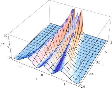
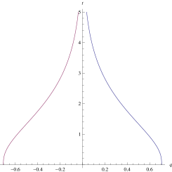
Figure 1: Case $\Omega^{2}=0.$ a) Evolution of probability density $\rho_{2}(q,t).$ b) Plot of moving zeros and poles.

6 Conclusion

In the present paper we have described time variable Madelung fluid and its linearization in terms of time variable linear Schrödinger equation. Our model, as descriptive of dissipative quantum fluid, admits exact solution for specific time dependent systems, like the harmonic oscillator with time dependent frequency and mass. In this case, exact time evolution has been described in terms of solutions for the corresponding damped classical oscillator. In particular, for the damping simulated by an exponentially growing mass (the Caldirola-Kanai model), it can be shown that the quantum damping squeezes the density function of the fluid and leads to Dirac-delta function. This can have some implications in quantum cosmology. In fact, if $\Psi(q,t)$ is a solution of the Caldirola-Kanai oscillator for a damped system

$$i\hbar\frac{\partial\Psi}{\partial t}=-\frac{\hbar^{2}}{2}e^{-\gamma t}\frac{\partial^{2}\Psi}{\partial q^{2}}+\frac{1}{2}\omega_{0}^{2}e^{\gamma t}q^{2}\Psi,$$

then $\,\,\Phi(q,t)=\Psi^{*}(q,-t),\,\,$ where $(*)$ denotes complex conjugation, is a solution of the related dual amplified system

$$i\hbar\frac{\partial\Phi}{\partial t}=-\frac{\hbar^{2}}{2}e^{\gamma t}\frac{\partial^{2}\Phi}{\partial q^{2}}+\frac{1}{2}\omega_{0}^{2}e^{-\gamma t}q^{2}\Phi.$$

Hence, knowing that the solution $\Psi(q,t)$ of the Caldirola-Kanai model has merging zeros and describes collapse of the wave function to Dirac-delta function at time infinity, leads to possible interpretation of the solution $\Psi^{*}(q,-t)$ for the dual system. Namely, we will have expanding wave function with creation of zeros as point particles from initial singularity at time zero. And this evolution simulates quantum mechanism similar to creation of expanding Universe from initial singularity in Big-Bang cosmology.

Finally, we note that by our results it is possible to find explicit exact solutions to a wide class of exactly solvable dissipative quantum fluids and complex Schrödinger-Burgers equations. For this we can use our recent work on exactly solvable dissipative systems, such as quantum Sturm-Liouville problems Ref.[7]. Then, it is possible also to describe the dynamics of the zeros and poles in the corresponding dissipative linear and nonlinear systems. These questions are under investigation now.

References

• [1] V.E. Zakharov, ”Dispersionless limit of integrable systems in 2+1 dimensions” in Singular Limit of Dispersive Waves (NATO Adv. Sci. Inst. Ser. B, Phys., Vol. 320, N.M. Ercolani et al., eds.), Plenum, New York (1994).
• [2] E. Madelung, Z. Phys. 40, 322 (1926).
• [3] P. R. Holland, The Quantum Theory of Motion, Cambridge University Press, (1993).
• [4] J.D. Cole, On a quasi-linear parabolic equation occuring in aerodynamics, Quart. Appl. Math., 9, 225 (1951).
• [5] E. Hopf, The partial differential equation $u_{t}+uu_{x}=u_{xx},$ Comm. Pure Appl. Math., 3, 201 (1950).
• [6] F. Calogero, Lett. Nuovo Cim. B43 (1978) 177-241; in Nonlinear equations in physics and mathematics. Barut A.O ed
• [7] Ş.A. Büyükaşık, O.K. Pashaev, E. Ulaş-Tigrak, J. Math. Phys, 50, 072102 (2009).
• [8] J. Wei, E. Norman, J. Math. Phys., 4, 575 (1963).
• [9] A. Perelomov, Generalized Goherent States and Their Applications, Springer-Verlag, (1986).
• [10] G. Dattoli, S. Solimeno, A. Torre, Phys. Rew. A, 34, 2646(1986).
• [11] P. Caldirola, Forze non conservative nella meccanica quantistica, Nouovo Cimento, 18, (1941).
• [12] E. Kanai, On the Quantization of the Dissipative Systems, Prog.Theo.Physics, 3, 440 (1948).
• [13] E.A. Galapon, J.Phys. A: Math. Theor., 42 (2009) 175201
• [14] I.M. Gelfand, G.E. Shilov, Generalized Functions, Vol.1, Academic Press, New York and London, 1964.
• [15] R.R. Parwani, O.K. Pashaev, J. Phys.A: Math and Theory, 41, 235207 (2008)
• [16] O.K. Pashaev, Jyh-Hao Lee, Abelian Gauge Theory and Integrable Sigma Models, Institute of Mathematics, Academia Sinica, Taiwan, (2000).
• [17] O.K. Pashaev, Relativistic Burgers and Non-linear Schrödinger Equations, Theor. Math. Phys, 160, 1023 (2009).