Correlation function and mutual information

Abstract

Correlation function and mutual information are two powerful tools to characterize the correlations in a quantum state of a composite system, widely used in many-body physics and in quantum information science, respectively. We find that these two tools may give different conclusions about the order of the degrees of correlation in two specific two-qubit states. This result implies that the orderings of bipartite quantum states according to the degrees of correlation depend on which correlation measure we adopt.

I Introduction

Entanglement is a kind of correlation in a quantum state of a composite system, which can not be simulated only with classical resources Wer89 . The research on entanglement has become a rich branch in the research of quantum information science HHHH09 . Comparing with entanglement, correlation functions have been proved to be useful concepts in describing the correlation effects in many-body physics. Since the correlation functions Ma85 are directly related with observables, they find many successful applications in many-body physics, e.g. correlation is a crucial element for understanding critical phenomena Wil75 .

A basic idea is to distinguish different types of correlations in a multipartite quantum state. For example, correlations in a quantum state can be classified into classical correlation and quantum correlation, and entanglement is contained in quantum correlation HV02 ; OZ02 ; GPW05 ; Luo08 ; Wal09 ; MPSVW10 . In quantum information science, the degree of (total) correlation in a composite quantum state is usually described mathematically by mutual information. Notice that correlation functions do not distinguish classical or quantum correlations either, correlation functions and mutual entropy describe the same (or similar) properties of the quantum state. Intuitively speaking, the larger the magnitude of the correlation function or the mutual entropy for a quantum state is, the more correlated the state is. Then the ordering of quantum states on the degrees of correlation can be built by comparing the magnitude of the correlation functions or the mutual entropy. A natural question is whether they give the same ordering of quantum states on the degrees of correlation.

This question is reminiscent of a similar situation when dealing with entanglement. The general concept of entanglement monotone is introduced to characterize the order on the degree of entanglement Vid00 . Different entanglement monotones may give different ordering of quantum states on the degrees of entanglement EP99 ; MG04 . This consideration motivates us to take a similar way to solve the present problem on correlation instead of entanglement.

In this article, we will perform a comparative study on the correlation functions and mutual information in characterizing the degree of correlation. This article is organized as follows. In Sec. II, we will briefly review two correlation measures, where the first one is directly related with the correlation functions. In Sec. III, we will compare the above two correlation measures on the classically correlated two-qubit states . In Sec. IV, we will give three relative discussions on the problem. Finally, we will give a brief summary.

II Two correlation measures

We consider a quantum state $\rho^{(12)}$ for a system composed by two subsystems $1$ and $2$. A correlation measure for the bipartite quantum state $\rho^{(12)}$, denoted as $C(\rho^{(12)})$, is a function that should satisfy four basic requirements HV02 ; ZZXY06 :

1. It is semi-positive, i.e. $C(\rho^{(12)})\geq 0$.

2. It is zero if and only if the two partite state $\rho^{(12)}$ is a product state, i.e. $C(\rho^{(12)})=0$ $\Leftrightarrow$ $\rho^{(12)}=\rho^{(1)}\otimes\rho^{(2)}$.

3. It is invariant under local unitary transformations, i.e. $C(U^{(1)}U^{(2)}\rho^{(12)}U^{(2)\dagger}U^{(1)\dagger})=C(\rho^{(12)})$.

4. It does not increase under local operations, i.e. $C(\mathcal{E}^{(1)}\mathcal{E}^{(2)}(\rho^{(12)}))\leq C(\rho^{(12)})$.

These four requirements, however, does not imply that there exists a unique correlation measure.

A possible way to construct a correlation measure is given as follows. For any given bipartite quantum state $\rho^{(12)}$, we can introduce a product state $\tilde{\rho}^{(12)}=\rho^{(1)}\otimes\rho^{(2)}$, where $\rho^{(1)}$ and $\rho^{(2)}$ are reduced density matrices of $\rho^{(12)}$ . Then we use different distance measures to characterize the difference between $\rho^{(12)}$ and $\tilde{\rho}^{(12)}$. By this way, we construct two correlation measures for a bipartite quantum state $\rho^{(12)}$. The first one ZZXY06 is

$$C_{I}(\rho^{(12)})=D(\rho^{(12)},\tilde{\rho}^{(12)}),$$ (1)

where the trace distance $D(\sigma,\tau)\equiv\frac{1}{2}\mathrm{\mathrm{Tr}}|\sigma-\tau|$ NC00 .

The second one is

$$C_{II}(\rho^{(12)})=S(\rho^{(12)}||\tilde{\rho}^{(12)}),$$ (2)

where the quantum relative entropy $S(\sigma||\tau)\equiv\mathrm{Tr}(\sigma(\ln\sigma-\ln\tau))$ is a distance-like function NC00 .

It is easy to prove that the two functions $C_{I}(\rho^{(12)})$ and $C_{II}(\rho^{(12)})$ satisfy the four basic requirements of a correlation measure, and thus both of them are legitimate correlation measures. A natural question arises: do these correlation measures give the same ordering on the degrees of correlations for all bipartite quantum states? Here the same order means the following equivalence relation: for any bipartite quantum states $\rho^{(12)}$ and $\sigma^{(12)}$,

$$C_{I}(\rho^{(12)})>C_{I}(\sigma^{(12)})\Longleftrightarrow C_{II}(\rho^{(12)})>C_{II}(\sigma^{(12)}).$$ (3)

The basic requirements of a correlation measure ensure that $C_{I}(\rho^{(12)})$ and $C_{II}(\rho^{(12)})$ will give the same order of correlation for some classes of bipartite quantum states. For example, if a bipartite state can be obtained by local operations on the other state, then all the measures of correlation will give the same order for these two states according to the fourth requirement.

Before investigating the above problem in detail, we first build a direct relation between correlation functions and the correlation measure $C_{I}$.

Correlation functions and $C_{I}$

To answer the question raised above, we find that it is sufficient to restrict our discussions to the two-qubit case. For a two-qubit system, the correlation function is defined by

$$C_{F}(\sigma_{i}^{(1)},\sigma_{j}^{(2)})=\mathrm{Tr}(\rho^{(12)}\sigma_{i}^{(1)}\sigma_{j}^{(2)})-\mathrm{Tr}(\rho^{(1)}\sigma_{i}^{(1)})\mathrm{\mathrm{Tr}(\rho^{(2)}\sigma_{j}^{(2)}),}$$ (4)

where $i,j\in\{x,y,z\}$. We observe that, on one hand, a correlation function $C_{F}(\sigma_{i}^{(1)},\sigma_{j}^{(2)})$ does not satisfy any basic requirement of a correlation measure, and it is not a legitimate correlation measure. On the other hand, if a two partite state is a product state, then the correlation function is zero. In this sense, a correlation function is the witness of correlation. Notice that

$$\rho^{(12)}-\rho^{(1)}\rho^{(2)}=\frac{1}{4}\sum_{i,j}C_{F}(\sigma_{i}^{(1)},\sigma_{j}^{(2)})\sigma_{i}^{(1)}\sigma_{j}^{(2)}.$$ (5)

Eq.(5) implies that the information of all the independent correlation functions are contained in the operator $\rho^{(12)}-\rho^{(1)}\rho^{(2)}$, which completely determines the correlation measure $C_{I}(\rho^{(12)})$. Therefore, the correlation measure $C_{I}(\rho^{(12)})$ is directly related with all the independent correlation functions.

III Comparisons of correlation measures

To compare the correlation measures $C_{I}(\rho^{(12)})$ and $C_{II}(\rho^{(12)})$, we consider a classically correlated two-qubit state Luo08 ; MPSVW10

$$\rho^{(12)}=p_{00}|00\rangle\langle 00|+p_{01}|01\rangle\langle 01|+p_{10}|10\rangle\langle 10|+p_{11}|11\rangle\langle 11|,$$ (6)

where $0\leq p_{00},p_{01},p_{10},p_{11}\leq 1$ and $p_{00}+p_{01}+p_{10}+p_{11}=1$.

A direct calculation gives that

$$C_{I}(\rho^{(12)})=2|p_{00}p_{11}-p_{01}p_{10}|,$$ (7)

and

$$C_{II}(\rho^{(12)}) = -(p_{00}+p_{01})\ln(p_{00}+p_{01})-(p_{10}+p_{11})$$ (8)

$$\times\ln(p_{10}+p_{11})-(p_{00}+p_{10})\ln(p_{00}+p_{10})$$

$$-(p_{01}+p_{11})\ln(p_{01}+p_{11})+p_{00}\ln p_{00}$$

$$+p_{01}\ln p_{01}+p_{10}\ln p_{10}+p_{11}\ln p_{11}.$$

For the two-qubit state (6), the unique nonzero correlation function is $C_{F}(\sigma_{z}^{(1)},\sigma_{z}^{(2)})$, and we have

$$C_{I}(\rho^{(12)})=\frac{1}{2}|C_{F}(\sigma_{z}^{(1)},\sigma_{z}^{(2)})|.$$ (9)

Eq. (7) and (8) show that the mathematical expressions for the two correlation measures are very different, and the relation between them is not simple. What are the similarities and differences between the two correlation measures? We will compare these two measures by numerical and analytical methods in the following subsections.

III.1 Numerical results

Since the two correlation measures $C_{I}$ and $C_{II}$ are the functions of three independent probabilities, we had better scan one probability to make they can be demonstrated in a $2$-dimensional figure. First, we scan the probability $p_{10}$, and show the results in Fig. 1.

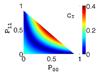
(a) $C_{I}$ when $p_{10}=0.1$.

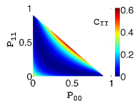
(b) $C_{II}$ when $p_{10}=0.1$.

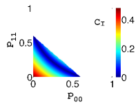
(c) $C_{I}$ when $p_{10}=0.4$.

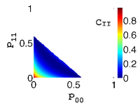
(d) $C_{II}$ when $p_{10}=0.4$.

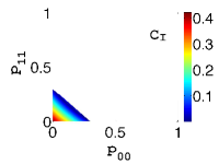
(e) $C_{I}$ when $p_{10}=0.7$.

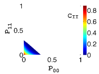
(f) $C_{II}$ when $p_{10}=0.7$.

Figure 1: Numerical comparison of $C_{I}$ and $C_{II}$ with varying $p_{10}$.

The numerical results in Fig. 1 show that these two measures give very similar behaviors. More precisely, $C_{I}$ and $C_{II}$ show the same increasing or decreasing behavior with varying the parameters.

To demonstrate the universality of the above observation, we further scan the probability $p_{11}$ to obtain the two correlation measures in Fig. 2. We find a similar behavior of the two correlation measures as those appeared in Fig. 1.

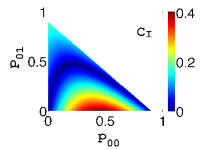
(a) $C_{I}$ when $p_{11}=0.1$.

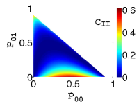
(b) $C_{II}$ when $p_{11}=0.1$.

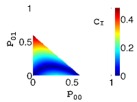
(c) $C_{I}$ when $p_{11}=0.4$.

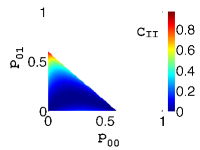
(d) $C_{II}$ when $p_{11}=0.4$.

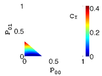
(e) $C_{I}$ when $p_{11}=0.7$.

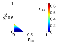
(f) $C_{II}$ when $p_{11}=0.7$.

Figure 2: Numerical comparison of $C_{I}$ and $C_{II}$ with varying $p_{11}$.

The numerical results in Fig. 1 and Fig. 2 show the similarities of these two measures, which supports that they both characterize the same quantity — the degree of correlation.

III.2 Analytical results

The above numerical results seem to support the validity of Eq. (3). However, we will prove the following proposition: there exist two quantum states such that Eq. (3) is no longer true.

Let us construct two quantum states that do not satisfy Eq. (3).

We take $p_{10}=\frac{1}{8}$ and $p_{11}=\frac{3}{8}$ in the quantum state (6). Then $p_{00}\in[0,\frac{1}{2}]$, and Eq. (7) and (8) become

$$C_{I}(p_{00})=|p_{00}-\frac{1}{8}|,$$ (10)

and

$$C_{II}(p_{00}) = p_{00}\ln p_{00}+(\frac{1}{2}-p_{00})\ln(\frac{1}{2}-p_{00})$$ (11)

$$-(\frac{1}{8}+p_{00})\ln(\frac{1}{8}+p_{00})-(\frac{7}{8}-p_{00})$$

$$\times\ln(\frac{7}{8}-p_{00})+\frac{3\ln 3-4}{8},$$

which are demonstrated in Fig. 3.

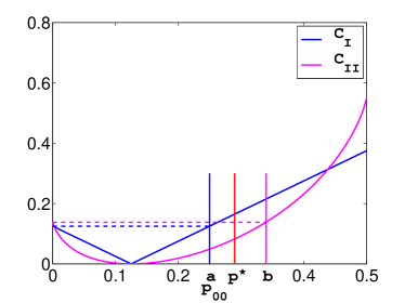
Figure 3: $C_{I}$ and $C_{II}$ varying with $p_{00}$ when $p_{10}=\frac{1}{8}$ and $p_{11}=\frac{3}{8}$.

A simple calculation gives that $C_{I}(0)=\frac{1}{8}$, $C_{I}(\frac{1}{8})=0$, $C_{I}(\frac{1}{2})=\frac{3}{8}$, $C_{II}(0)=2+\frac{3\ln 3-7\ln 7}{8}$, $C_{II}(\frac{1}{8})=0$, and $C_{II}(\frac{1}{2})=2-\frac{5\ln 5}{8}$. It is easy to check that $C_{I}(\frac{1}{8})<C_{I}(0)<C_{I}(\frac{1}{2})$ and $C_{II}(\frac{1}{8})<C_{II}(0)<C_{II}(\frac{1}{2})$. We can also prove that $C_{I}(p_{00})$ and $C_{II}(p_{00})$ are continuous strictly increasing function when $p_{00}\in[\frac{1}{8},\frac{1}{2}]$. According to the intermediate value theorem, there exist $a,b\in[\frac{1}{8},\frac{1}{2}]$, such that $C_{I}(a)=C_{I}(0)$ and $C_{II}(b)=C_{II}(0)$.

We will prove that $a<b$. It is easy to observe that $C_{I}(\frac{1}{4})=C_{I}(0)=\frac{1}{8}$, so $a=\frac{1}{4}$. A direct calculation gives

$$C_{II}(\frac{1}{4})-C_{II}(0)=\frac{1}{8}\ln\frac{823543}{1350000}<0,$$

which implies that $C_{II}(\frac{1}{4})<C_{II}(0)=C_{II}(b)$. Since the function $C_{II}$ is strictly increasing function when $p_{00}\in[\frac{1}{8},\frac{1}{2}]$, we have $a=\frac{1}{4}<b$.

$\forall p^{\star}\in(a,b)$, we have

$$C_{I}(0)=C_{I}(a)<C_{I}(p^{\star}),$$ (12)

$$C_{II}(0)=C_{II}(b)>C_{II}(p^{\star}).$$ (13)

In Eqs. (12) and (13), we use the fact again that $C_{I}$ and $C_{II}$ are strictly increasing functions when $p_{00}\in[\frac{1}{8},\frac{1}{2}]$. This completes our proof of the proposition.

IV Discussions

First, we will address one aspect in the relations between correlation and entanglement. Since entanglement is a kind of quantum correlation, it is interesting to ask whether the appearance of entanglement can be identified in the degree of correlation. Here we will try to give an answer with the Werner states Wer89 , which are defined by

$$\rho_{W}(F)=\frac{1-F}{3}I^{(1)}I^{(2)}+\frac{4F-1}{3}|\Psi^{-}\rangle\langle\Psi^{-}|,$$ (14)

where $0\leq F\leq 1$ and $|\Psi^{-}\rangle=\frac{1}{\sqrt{2}}(|01\rangle-|10\rangle)$. As is well known, the Werner states are entangled if and only if $F>\frac{1}{2}$ BDSW96 . The expressions for the two correlation measures are given respectively by

$$C_{I}(\rho_{W}(F))=|F-\frac{1}{4}|,$$ (15)

and

$$C_{II}(\rho_{W}(F))=\ln\frac{4}{3}+F\ln 3+F\ln F+(1-F)\ln(1-F),$$ (16)

which are numerically demonstrated in Fig. 4.

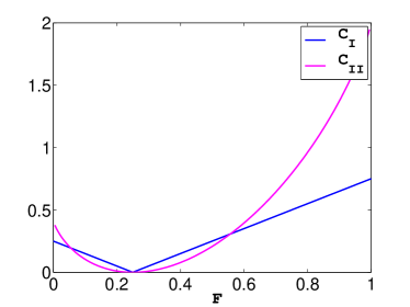
Figure 4: The two correlation measures for the Werner states.

As shown in Fig. 4, there is not any evidence in the two correlation measures that shows the appearance of entanglement at $F=\frac{1}{2}$.

Second, the two correlation measures are related by the following inequalities NC00 ; OP93 ; WVHC08 :

$$2C_{I}^{2}(\rho^{(12)})\leq C_{II}(\rho^{(12)})\leq 2C_{I}(\rho^{(12)})\ln d+\frac{1}{e},$$ (17)

where $d$ is the dimension of the Hilbert space of the composite system. When $2C_{I}(\rho^{(12)})\leq\frac{1}{e}$, the right part of the inequality (17) can be strengthened to

$$C_{II}(\rho^{(12)})\leq 2C_{I}(\rho^{(12)})\ln d-2C_{I}(\rho^{(12)})\ln(2C_{I}(\rho^{(12)})).$$ (18)

The inequalities (17) and (18) show that we can estimate the range of values taken by $C_{II}$ from the value of $C_{I}$.

Third, in addition to the two correlation measures $C_{I}$ and $C_{II}$, there exist other correlation measures, e.g.

$$C_{III}(\rho^{(12)})=A(\rho^{(12)},\tilde{\rho}^{(12)}),$$ (19)

where the angle distance $A(\sigma,\tau)\equiv\arccos F(\sigma,\tau)$ with the fidelity $F(\sigma,\tau)\equiv\mathrm{Tr}\sqrt{\sigma^{\frac{1}{2}}\tau\sigma^{\frac{1}{2}}}$ NC00 . In this measure, the fidelity $F(\rho^{(12)},\tilde{\rho}^{(12)})$ plays a central role. In fact, we can construct a correlation measure directly from the Fidelity by

$$C_{III}^{\prime}(\rho^{(12)})=1-F^{2}(\rho^{(12)},\tilde{\rho}^{(12)}).$$ (20)

It is easy to prove that $C_{III}(\rho^{(12)})$ and $C_{III}^{\prime}(\rho^{(12)})$ will give the same order on the degree of correlation for any two partite quantum states.

V Summary

We briefly review two different correlation measures for a bipartite quantum state, and associate the first correlation measure with the correlation functions. Comparing these two correlation measures for the classically correlated two-qubit states, we observe that they give the same ordering on the degrees of correlation for most quantum states. However, we find that the two correlation measures can give different orderings on the degrees of correlations for some two specific two-qubit states. This situation is similar to the work on entanglement monotone, where different entanglement monotones may give different orderings of two quantum states on the degree of entanglement. Our work present a comparison between the correlation functions and mutual information on characterizing the degrees of correlation in multipartite quantum states , which sheds a novel light on the interplay between many-body physics and quantum information science.

Acknowledgments: This work is supported by NSF of China under Grant No. 10775176 and 10975181, and NKBRSF of China under Grants No. 2006CB921206.

References

- (1) R. Werner, Phys. Rev. A 40, 4277 (1989)
- (2) R. Horodecki, P. Horodecki, M. Horodecki, and K. Horodecki, Rev. Mod. Phys. 81, 865 (2009)
- (3) S. Ma, Statistical Mechanics (World Scientific Publishing Co. Pte. Ltd., Singapore, 1985)
- (4) K. Wilson, Rev. Mod. Phys. 47, 773 (1975)
- (5) L. Henderson and V. Vedral, J. Phys. A 34, 6899 (2000)
- (6) H. Ollivier and W. Zurek, Phys. Rev. Lett. 88, 017901 (2002)
- (7) B. Groisman, S. Popescu, and A. Winter, Phys. Rev. A 72, 032317 (2005)
- (8) S. Luo, Phys. Rev. A 77, 022301 (2008)
- (9) Z. Walczak, Phys. Lett. A 373, 1818 (2009)
- (10) K. Modi, T. Paterek, W. Son, V.Vedral, and M. Williamson, Phys. Rev. Lett. 104, 080501 (2010)
- (11) G. Vidal, J. Mod. Opt. 47, 355 (2000)
- (12) J. Eisert and M. Plenio, J. Mod. Opt. 46, 145 (1999)
- (13) A. Miranowicz and A. Grudka, J. Opt. Soc. Am. B 6, 542 (2004)
- (14) D. L. Zhou, B. Zeng, Z. Xu, and L. You, Phys. Rev. A 74, 052110 (2006)
- (15) M. A. Nielsen and I. Chuang, Quantum Computation and Quantum Information (Cambridge University Press, Cambridge, 2000)
- (16) C. Bennett, D. Divincenzo, J. Smolin, and W. Wootters, Phys. Rev. A 54, 3824 (1996)
- (17) M. Ohya and D. Petz, Quantum Entropy and its Use (Springer, Heidelberg, 1993)
- (18) M. Wolf, F. Verstraete, M. Hastings, and J. Cirac, Phys. Rev. Lett. 100, 070502 (2008)