Gluon emission in Quark-Gluon Plasma

Abstract

Gluon radiation is an important mechanism for parton energy loss as the parton traverses the quark gluon plasma (QGP) medium. We studied the gluon emission in QGP using AMY formalism. In the present work, we obtained gluon emission amplitude F(h,p,k) function , which is a solution of the integral equations describing gluon radiation including Landau-Pomeranchuk-Migdal (LPM) effects, using iterations method. We define a new dynamical scale for gluon emission denoted by $x$. The gluon emission rate is obtained by integrating these amplitude function over h. We show that these obey a simple scaling in terms of this dynamical variable $x$. We define the gluon emission function $g(x)$ for gluon radiation for the three processes $g\rightarrow gg$,$q\rightarrow gq$ and $g\rightarrow q\bar{q}$. In terms of this $g(x)$ function, the parton energy loss calculations, due to medium induced gluon radiation, may become simplified.

Lattice quantum chromo dynamics (LQCD) calculations karsch predict a transition from confined state in hadrons to a deconfined state of quarks and gluons above a temperature of 170 MeV or an energy density above 1GeV/fm³ . In the relativistic heavy ion collisions at RHIC at BNL with an energy density above 5GeV/fm³, experimental measurements of several observables indicate such a transition to a deconfined state of matter brahms ; phobos ; star ; phenix , for details see the reviews emsig ; qgpreview ; rapp ; enteria . It is currently believed that this deconfined state consists of a strongly interacting Quark Gluon Plasma (sQGP), behaving nearly like a perfect liquid qgpreview . Among these observables, jet-quenching phenomenon is so far an important signal for a hot dense medium formed. Jet suppression has its origin in parton energy loss in the quark matter by gluon radiation, which distinctly differs from energy loss in hadronic matter. For example the suppression of high-$p_{T}$ pions, from 3GeV to 10GeV, of BNL experiments can be explained by assuming a deconfined state.
We studied gluon radiation problem as this has direct application to the energy loss of partons while traversing the QGP medium due to the gluon bremsstrahlung processes. In addition to radiation, the elastic energy loss of partons traversing the QGP medium is important for heavy quark quenching, observed in RHIC experiments. For an exposition of theoretical and experimental results on parton energy loss the readers may see an excellent review mazum .
In the present work, we study the gluon radiation mechanism. The coherent radiation processes involve multiple scatterings of the partons in the QGP medium during the gluon formation time. This leads to interference effects known as Landau-Pomeranchuk-Migdal effect (LPM). Gluon emission is discussed widely in literature baier -moore1 . These works treated the parton energy loss on the basis of avarage energy loss dependeing on the path length. As emphasized in moore2 , the bremsstrahlung (gluon emission), is characteristically different in the sense that it is a stochastic process. Starting with a group of partons of fixed energy, the bremsstrahlung process results in a broad spectrum of final partons of width comparable to its mean energy loss. Further, the LPM effect has different parametric dependence on energy for soft and hard parts of emitted gluon spectrum. As compared to the case of bremsstrahlung photon emission, the gluon emission also involves an enhancement mechanism when the emitted gluon and quark are nearly collinear, thereby a need to consider ladder diagrams amy3 . However, unlike the emission of electromagnetic quanta, the emitted hard gluon feels the random colored background field. The resummation of these ladder diagrams leads to Swinger-Dyson type integral equations. In this work, we follow the formalism given in amy3 -moore2 which implements LPM effects by resumming the ladder diagrams. For calculating parton energy loss arising from gluon radiation, one needs the differential gluon emission rates and this is given by Eq.1 moore2 in terms of the F(h,p,k) function. The bremsstrahlung integral equations determine the gluon emission amplitude F(h,p,k) function given by Eq.2. Here, the two dimensional vector $\bf{h}=p\times k$ is of the order of $O(gT^{2})$. It is a measure of collinearity and its magnitude is small compared to $\bf{pk}$. The term $\delta{E}({\bf{h}},p,k)$ in Eq.2 is the energy differential between initial and final states. Here, $m_{k}^{2}=m_{D}^{2}/2=2g^{2}T^{2}/3$ and other quark thermal masses are $m^{2}=g^{2}T^{2}/3$. This formalism is very similar to the photon emission integrals, however, as mentioned before, the emitted gluon has color and therefore interacts with other scattering centers as well as soft background fields amy3 . Accordingly, there are three terms in the integral equations of 2 involving collision kernel $C({\bf{h}})$. A typical ladder diagram for gluon emission is shown in Figure 1. We solve this integral equation for F(h,p,k) function, by using iterations method as discussed in surya1 . The F(h,p,k) distributions for various values of parton and gluon momenta (p,k) were obtained considering the mechanism $g\rightarrow gg$, $q\rightarrow gq$ and $g\rightarrow q\bar{q}$ processes using relevant factors ($N_{s}=2,d_{s}=d_{A}(=8)$, and $C_{s}=C_{A}(=3),C_{F}=4/3$). Fig.2 shows a few ${\bf F}({\bf h},p,k)$ distributions for these two processes (for high parton momenta) for various values of parton and gluon momenta (p,k). The real part is shown in figure (a) and negative of imaginary part in figure (b). Fig.2(c) shows the real part of the distributions for $g-gg$ process for high and low values of incoming and outgoing gluon momenta (p,k). The calculations for $g\rightarrow q\bar{q}$ process are shown in Fig.3. In all these figures, $p$ always stands for the incoming parton momentum.

$$\frac{d\Gamma_{g}^{LPM}}{d^{3}{\bf{k}}} = \frac{\alpha_{s}}{4\pi^{2}k^{2}}\sum_{s}N_{s}d_{s}C_{s}\int_{-\infty}^{+\infty}\frac{dp}{2\pi}\int\frac{d^{2}{\bf h}}{4\pi^{2}}$$ (1)

$$n_{s}(p+k)[1\mp n_{s}(p)][1+n_{b}(k)]$$

$$\frac{1}{k^{3}}|\Gamma^{s}_{p\rightarrow p+k}|^{2}2{\bf{h}}\cdot\Re{\bf{F}}_{s}({\bf{h}};p,k)~{}~{}~{}~{}~{}$$

$$2{\bf{h}} = {i}\delta{E}({\bf{h}},p,k){\bf{F(h)}}+g^{2}\int\frac{d^{2}{\bf{h}}}{(2\pi)^{2}}C({\bf{h}})$$ (2)

$$\times\left\{(C_{s}-C_{A}/2)\left[{\bf{F(h)}}-{\bf{F}}({{\bf{h}}}-k{\bf{h}})\right]\right.$$

$$\left.+(C_{A}/2)\left[{\bf{F(h)}}-{\bf{F}}({{\bf{h}}}+p{\bf{h}})\right]\right.$$

$$\left.+(C_{A}/2)\left[{\bf{F(h)}}-{\bf{F}}({{\bf{h}}}-(p-k){\bf{h}})\right]\right\}~{}~{}~{}~{}~{}$$

$$\delta{E}({\bf{h}},p,k) = \frac{{\bf{h^{2}}}}{2pk(p-k)}$$ (3)

$$+\left[\frac{m_{k}^{2}}{2k}+\frac{m_{p-k}^{2}}{2(p-k)}-\frac{m_{p}^{2}}{2p}\right]~{}~{}~{}~{}~{}~{}~{}~{}~{}$$

$${C}({\bf{h}}) = \frac{1}{\bf{h}^{2}}-\frac{1}{({\bf{h}^{2}}+1)}$$ (4)

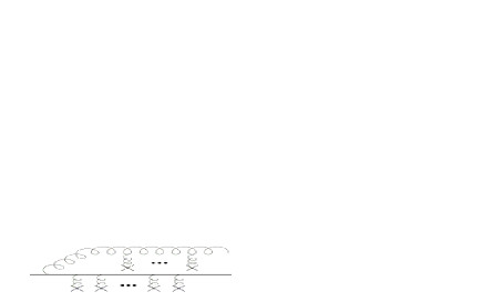
Figure 1: gluon radiation processes that contribute at order ${\alpha_{s}}$.

I Generalized Emission Functions for gluon emission

Before we discuss the emission functions for gluon emission, it is very instructive to recall the emission functions for photon emission. In our previous works surya1 ; svsprc , we showed generalized photon emission function by integrating (Eq.5) the corresponding ${\bf p_{\perp}{\cdot}f(p_{\perp})}$ distributions (see surya1 .

$$I_{T} = \int\frac{\bf d^{2}\tilde{p}_{\perp}}{(2\pi)^{2}}{\bf\tilde{p}_{\perp}{\cdot}\Re\tilde{f}(\tilde{p}_{\perp})}$$ (5)

$$x_{0} = \frac{|(p_{0}+q_{0})p_{0}|}{q_{0}T}$$ (6)

$$x_{1} = x_{0}\frac{M_{\infty}^{2}}{m_{D}^{2}}$$ (7)

$$x_{T} = x_{1}+x_{2}$$ (8)

$$g(x) = I\times c$$ (9)

$$c = \frac{1}{x_{1}^{2}}$$ (10)

$$g^{b}_{T}(x) = \frac{10.0}{5.6+2.5\sqrt{x}+x}$$ (11)

$$\Im{\Pi^{\mu}}_{R\mu} = \frac{e^{2}N_{c}}{2\pi}\int_{-\infty}^{\infty}dp_{0}[n_{F}(r_{0})-n_{F}(p_{0})]\otimes$$ (12)

$$\left(Tm_{D}^{2}\right)\left[\frac{p_{0}^{2}+r_{0}^{2}}{2(p_{0}r_{0})^{2}}\left(\frac{g^{i}_{T}\left(x_{T}\right)}{c^{i}_{T}}\right)+\right.$$

$$\left.\frac{1}{\sqrt{\left|p_{0}r_{0}\right|}}\frac{Q^{2}}{q^{2}}\left(\frac{1}{m_{D}}\right)\left(\frac{g^{i}_{L}\left(x_{L}\right)}{c^{i}_{L}}\right)\right]$$

$I$ are in general functions of {$p_{0},q_{0},Q^{2},T,\alpha_{s}$} and therefore, we defined the generalized emission functions (GEF) $g$ in Eq.9, which are functions of only $x$ variables. These GEF ($g$) are obtained from corresponding $I$ values by multiplying with $c$ coefficient functions given in surya1 . As an example, in Figure 4, we show the results for GEF for bremsstrahlung (Fig.4(a)). The solid curve in (a) is the empirical fit to this emission function, given by Eq.11. Consequent to finding the emission functions like those given by Eq.11, we expressed the imaginary part of retarded photon polarisation tensor for any $p_{0},q_{0},Q^{2},T,\alpha_{s}$ values by using Eq.12. Using this approach, we obtained the phenomenological fits to virtual photon emission rates from QGP for ladder processes with LPM effects surya1 . We provided simple phenomenological formulae which are useful in model calculations for experimental dilepton yields.

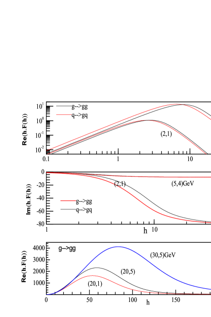
Figure 2: (a) Shows the real part of ${\bf h}$ distributions of the ${\bf h}\cdot{\bf\Re{F}}({\bf h})$ for gluons. Various curves are for various parton momenta (p) and gluon momenta (k) values as mentioned in figure labels as (p,k). The distributions are obtained using iterations method.
(b) Shows the imaginary part of ${\bf h}$ distributions of the ${\bf h}\cdot{\bf\Im{F}}({\bf h})$
(c) Shows the real part of ${\bf h}$ distributions of the ${\bf h}\cdot{\bf\Re{F}}({\bf h})$ for pure glue process. Various curves are for various parton momenta (p) and gluon momenta (k) values as mentioned in figure labels as (p,k).

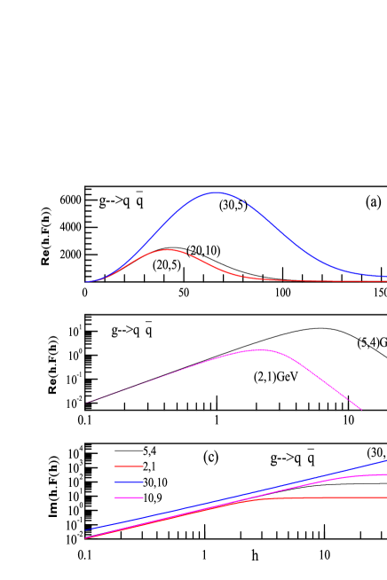
Figure 3: (a) Shows the real part of ${\bf h}$ distributions of the ${\bf h}\cdot{\bf\Re{F}}({\bf h})$ for $g\rightarrow q\bar{q}$ process. Various curves are for various gluon momenta (p) and quark momenta (k) values as mentioned in figure labels as (p,k). The distributions are obtained using iterations method.
(b) Shows the real part of ${\bf h}$ distributions of the ${\bf h}\cdot{\bf\Re{F}}({\bf h})$ for $g\rightarrow q\bar{q}$ process. Various curves are for various gluon momenta (p) and quark momenta (k) values as mentioned in figure labels as (p,k).
(c) Shows the imaginary part of ${\bf h}$ distributions of the ${\bf h}\cdot{\bf\Im{F}}({\bf h})$

Figure 4: (a)  The dimensionless emission function $g^{b}_{T}(x)$ versus dynamical variable $x_{T}$ defined in Eq.8. Six cases of temperature and coupling constant values considered are mentioned in figure labels in different type symbols. The symbols represent the integrated values of ${\bf p_{\perp}}$ distributions as a function of $\{p_{0},q_{0},Q^{2},T,\alpha_{s}\}$ values. The solid curve is an empirical fit given by Eq.11.

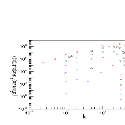
Figure 5:  The integral of gluon h distributions shown in previous figures for the process $g\rightarrow gg$. $\int\frac{\bf d^{2}{h}}{(2\pi)^{2}}{\bf h}\cdot{\bf\Re{F}}({\bf h})$ versus emitted gluon momentum (k). Here incoming parton momenta (in the present case, gluon momenta p) has not yet been integrated. The different parton momentum (gluon $p$) values are shown on the figure and temperature of plasma is taken T=1.0GeV.

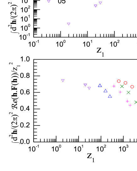
Figure 6:  The integral of gluon h distributions for the process $g\rightarrow gg$. The plot shows $\int\frac{\bf d^{2}{h}}{(2\pi)^{2}}{\bf h}\cdot{\bf\Re{F}}({\bf h})$ versus the variable z₁. The different parton momentum (gluon $p$) values are shown on the figure and temperature of plasma is taken T=1.0GeV.

Following the procedure of generalized photon emission function, we now try to obtain the generalized gluon emission functions. For this, we integrate these distributions, that have been shown in Figs.2,3 over the variable $\bf h$, as given in Eq.13. This quantity $I$ is strongly process dependent and is a function incoming and outgoing parton momenta, plasma temperature and strong coupling strength as denoted by the variables $p,k,T$ and $\alpha_{s}$. The integrated quantity $I$ is plotted versus $k$ in Figure 5 for the process $g\rightarrow gg$. Figure shows $I$ plotted for different values of $p$ labeled on the figure. As seen in figure, the $I$ values are scattered. Therefore, we defined a variable $z_{1}$ as given in Eq.14. We show $I$ values versus $z_{1}$ variable in figure 6. As seen in figure (a), it exhibits a linear behavior on log-log plot, extending over nine orders of magnitude. This apparently gives an impression that $z_{1}$ is a good dynamical scale for the process $g\rightarrow gg$. In order to examine this, we plot $I/z_{1}^{2}$ in figure (b). As seen in figure (b), the $I/z_{1}^{2}$ values are scattered and exhibit no useful trends, showing that $z_{1}$ is not a dynamical variable for this process. Therefore, we now define the dynamical variable $x$ and a function $g$, for $g\rightarrow gg$ process as given in Eqs.15,16. In the Fig.17, we show the function $g$ versus $x$. As seen in figure, all $I$ values for different parton momenta merge. We fit this data with an empirical curve together with parameters as given in Eqs.17,19. We denote this function in Eq.17 as gluon emission function for the process $g\rightarrow gg$.

We carried out this for the processes $q\rightarrow gq$ and $g\rightarrow q\bar{q}$. The $I$ values for these two processes also donot exhibit any trends as a function $z_{1}$ variable, however, $x$ remains a good dynamical variable. We show these results for the process $q\rightarrow gq$ in Fig.8 versus $x$. The curve in this figure is given by empirical fit and parameters in Eqs.20,23. Therefore, for $q\rightarrow gq$ , we define gluon emission function $g(x)$ as given in Eq.20. We performed these calculations for the process $g\rightarrow q\bar{q}$ and these results are shown in Fig.9. The curve in this figure is given by empirical fit and parameters in Eq.24,29. Therefore, for the process $g\rightarrow q\bar{q}$ , we define gluon emission function $g(x)$ as given in Eq.24.
After obtaining the gluon emission function $g(x)$ for these three processes, we can perform $p$ integrations required in Eq.1, i.e. integration in terms of dynamical variables $x$. This will give us differential gluon emission rates. In the jet-quenching studies, one needs to estimate the energy loss of high energy partons while traversing the QGP medium. In this problem, the differential gluon emission rates estimated by integrating over $p$ variable, will have to be coupled in order to determine the differential energy loss. These results were already shown by amy3 ; moore1 ; moore2 ; mazum .
In the following, we examine the integrand of differential gluon emission rate of the Eq.1, i.e., without $p$ integration, and we denote this in short by gluon rate, which should not be confused with the gluon emission rates after integrating over $p$. We obtained the $I$ values by integrating the $h$ distributions $\int\frac{\bf d^{2}{h}}{(2\pi)^{2}}{\bf h}\cdot{\bf\Re{F}}({\bf h})$. The splitting function $\left|\Gamma^{s}_{p\rightarrow p+k}\right|^{2}$ are as given in moore2 . In the Fig.10, we show the $I$ values (red curves), splitting function (blue curves) and the gluon rate (black curves) at three different $p$ values for the process $g\rightarrow gg$. We show similar results for the process $q\rightarrow gq$ in Fig.11 and for the process $g\rightarrow q\bar{q}$ in Fig.12.

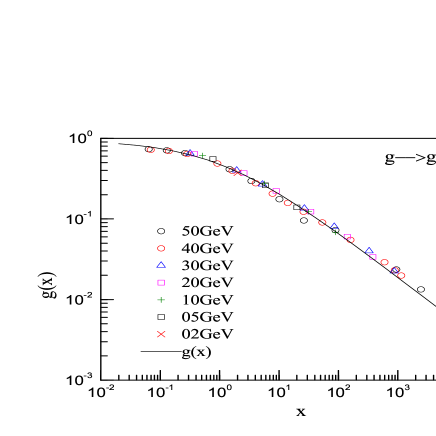
Figure 7:  The integral of gluon ${\bf h}$ distributions for the process $g\rightarrow gg$. The plot shows $\int\frac{\bf d^{2}{h}}{(2\pi)^{2}}{\bf h}\cdot{\bf\Re{F}}({\bf h})$ versus the new variable $x$. As before, different incoming parton momentum (gluon $p$) values are shown on the figure and temperature of plasma is taken T=1.0GeV.

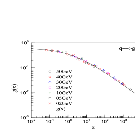
Figure 8:  The integral of gluon h distributions for the process $q\rightarrow gq$. This plot shows $\int\frac{\bf d^{2}{h}}{(2\pi)^{2}}{\bf h}\cdot{\bf\Re{F}}({\bf h})$ versus the new variable $x$. As before, incoming parton momentum (quark $p$) values are shown on the figure and temperature of plasma is taken T=1.0GeV.

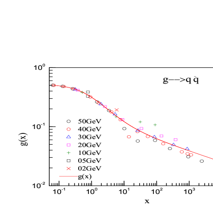
Figure 9:  The integral of gluon h distributions for the process $g\rightarrow q\bar{q}$. This plot shows $\int\frac{\bf d^{2}{h}}{(2\pi)^{2}}{\bf h}\cdot{\bf\Re{F}}({\bf h})$ versus the new variable $x$. The different incoming parton momentum (gluon $p$) values are shown on the figure and temperature of plasma is taken T=1.0GeV.

$$I = \int\frac{\bf d^{2}{h}}{(2\pi)^{2}}{\bf h}\cdot{\bf\Re{F}}({\bf h})$$ (13)

$$z_{1} = \left|\frac{(p-k)pk}{T}\right|$$ (14)

$$x = \frac{z_{1}}{{k^{2.35}}}$$ (15)

$$g = \frac{I}{z_{1}^{2}}\left(\frac{k}{p}\right)$$ (16)

$$g(x) = \frac{0.9500}{(1.000+cx^{w1})}$$ (17)

$$c = 0.995328684841907$$ (18)

$$w1 = 0.565842143207086$$ (19)

$$g(x) = \frac{a}{(1.000+cx^{w1})}$$ (20)

$$a = 0.609492873517025$$ (21)

$$c = 0.725062591204554$$ (22)

$$w1 = 0.533208076507815$$ (23)

$$g(x) = \frac{(a+bx^{w1})}{(1+cx^{w2})}$$ (24)

$$a = 0.51922$$ (25)

$$b = 0.185609$$ (26)

$$c = 1.21859$$ (27)

$$w1 = 0.807358$$ (28)

$$w2 = 1.00605$$ (29)

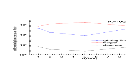
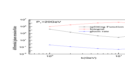
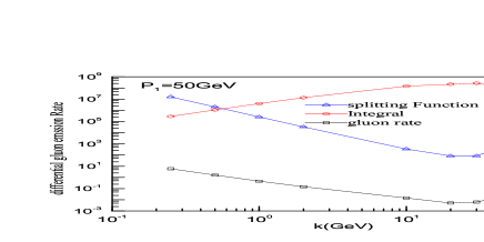
Figure 10:   Black line versus gluon momentum (k) shows the integrand (without p integration) of the differential gluon emission rate of Eq.1 $\frac{d\Gamma_{g}^{LPM}}{d^{3}{\bf{k}}}$ for the process $g\rightarrow gg$. The blue curve represents the splitting function for $g\rightarrow gg$ given by $|\Gamma^{s}_{p\rightarrow p+k}|$ of Eq.1 and the red curve represents the integral value $\int\frac{d^{2}{\bf h}}{(2\pi)^{2}}2{\bf{h}}\cdot\Re{\bf{F}}_{s}({\bf{h}};p,k)$. The incoming parton (gluon in this case) momentum $p$ (labeled as $p_{1}$ in figure) for this figure is fixed $p=10,20,50$GeV as indicated on the figure. Temperature of plasma is T=1.0GeV.

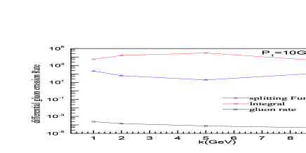
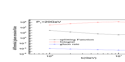
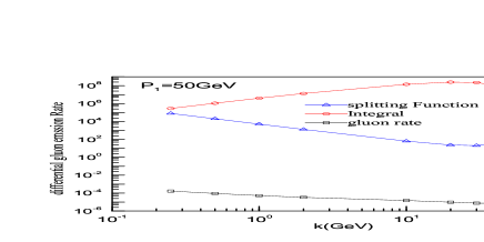
Figure 11:   Black line versus gluon momentum (k) shows the integrand of the differential gluon emission rate of Eq.1 $\frac{d\Gamma_{g}^{LPM}}{d^{3}{\bf{k}}}$ for the process $q\rightarrow gq$. The curves are as in Figure 10.

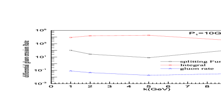
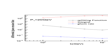
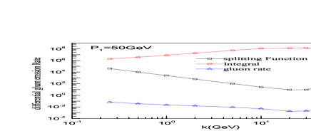
Figure 12:   Black line versus quark momentum (k) shows the integrand of differential emission rate of Eq.1 $\frac{d\Gamma_{g}^{LPM}}{d^{3}{\bf{k}}}$ for the process $g\rightarrow q\bar{q}$. The details are as in Figure 10.

In conclusion, the gluon emission in quark gluon plasma including LPM effects has been studied at a fixed temperatures and strong coupling strength. We defined a new dynamical variable $x$ for gluon emission. Further, we defined gluon emission functions (GEF) denoted by $g(x)$ for the processes $g\rightarrow gg$, $q\rightarrow gq$ and $g\rightarrow q\bar{q}$. We have obtained empirical fits to these GEF and provide the functional forms and parameters for all the three processes. We compared the differential gluon emission rates (without p-integration) for these three processes.
In terms of the GEF, we may calculate the differential gluon emission rates for these processes. These empirical formulae will be useful in calculations of parton energy loss by medium induced gluon radiation.

References

(1)F. Karsch, Nucl. Phys. A 698, 199 (2002).
(2) I. Arsene et al., [BRAHMS Collaboration], Nucl. Phys. A 757, 1 (2005), [nucl-ex/0410020v1]
(3)B.B. Back et al.,[PHOBOS Collaboration], Nucl. Phys. A 757, 28 (2005)
(4)J. Adams et al., [STAR Collaboration],Nucl. Phys. A 757, 102 (2005)
(5)K. Adcox et al., [PHENIX Collaboration],Nucl. Phys. A 757, 184 (2005)
(6)G. David, R. Rapp and Z. Xu, nucl-ex/0611009.
(7)David d’Enterria, Journ. of Phys. G34, S53 (2007) , [nucl-ex/0611012]
(8) G. David, R. Rapp, and Z. Xu, nucl-ex/0611009v2.
(9) David d’Enterria, J. Phys. G 34, S53 (2007), topical review.
(10) A. Mazumder and M . Van Leeuwen ArXiv:1002.2206v2 [hep-ph], 10 Feb 2010.
(11) R. Baier, D. Schiff and B. G. Zakharov, Ann. Rev. Nucl. Part. Sci. 50, 37 (2000) [hepph/0002198].
(12) B. G. Zakharov, [hep-ph/9807396]; JETP Lett. 73, 49 (2001) ,[hep-ph/0012360].
(13) R. Baier, Y. L. Dokshitzer, S. Peigne and D. Schiff, Phys. Lett. B 345, 277 (1995)
[hep-ph/9411409]; Phys. Rev. C 60, 064902 (1999) [hep-ph/9907267].
(14) R. Baier, Y. L. Dokshitzer, A. H. Mueller, S. Peigne and D. Schiff, Nucl. Phys. B 483,
291 (1997) [hep-ph/9607355]; ibid. 484, 265 (1997) [hep-ph/9608322].
(15) M. Gyulassy and X. n. Wang, Nucl. Phys. B 420, 583 (1994) [nucl-th/9306003].
(16) P. Arnold, G. D. Moore, and L. G. Yaffe, J. High Energy Phys., 0301, (2003) 030.
(17) Sangyong Jeon, and Guy D. Moore,Phys. Rev. C 71, (2005) 034901.
(18) Simon Turbide, et. al., Phys. Rev. C 72, (2005) 014906.