DESY 10–067
SFB/CPP–10–40
HEPTOOLS 10–018
Calculating multileg one-loop processes. The case of $gg\rightarrow t\bar{t}gg$

Abstract:

This study is targeted to the NLO corrections of multileg processes, very important for the LHC. Starting from the construction of Feynman diagrams, the analytical reduction of general one-loop integrals to scalar master ones, the calculation of color structures, manipulation of spinor lines and other amplitude constituents and finally phase space point selection are obtained by use of a program producing Fortran code for numerical calculation of one-loop corrections for processes like $gg\rightarrow t\bar{t}gg$.

1 Introduction

The era of LHC has finally arrived, after many years of waiting and anticipating, and all the particle physics community is waiting for the first results. There has been a lot of activity the last two years in the branch of NLO calculation. With almost all interesting cases of $2\rightarrow 3$ processes having been calculated, the interest has moved towards $2\rightarrow 4$. Processes like $pp\rightarrow t\bar{t}+b\bar{b}$ [1, 2, 3], $V+3jet$ production [4, 5, 6, 7], $qq\rightarrow b\bar{b}b\bar{b}$ [8] and most recently the case of $pp\rightarrow t\bar{t}+2jets$ [9] have been studied in the last three years, providing the background for future discoveries. This study is also towards this direction.

2 The method

Our method is based on the Feynman diagrammatic approach. Which means that we calculate the total amplitude by taking into consideration the contributions of each of the one-loop Feynman diagrams that exist for the NLO calculation. The final program calculating the amplitude is in Fortran, although a variety of tools are used in combination (see Figure 2): Diana [10] for constructing the diagrams, Form [11] for manipulation of the Diana output (the steps of calculation in Form are colored red), Maple for optimization of the produced Fortran code (green color) and finally Fortran for the numerical evaluation (blue color). In the next session we will explain in more detail the complete calculation, which ends by providing the amplitude from an initial phase space point.

2.1 The steps of the calculation

As mentioned above, the first step is implemented by using Diana. We provide the program with the appropriate Feynman rules and ask for the construction of diagrams. For the case of $gg\rightarrow t{\bar{t}}gg$ the total number of diagrams is 4510. Diana provides us with an output in Form which we further manipulate. The next step is to strip the one-loop amplitude from the color structures. In a few words using Form to manipulate the output of Diana we strip off and manipulate the color structures using color Algebra. We translate the Form result to Fortran code and end up with a Fortran array containing all the possible color information. For the case of $gg\rightarrow t{\bar{t}}gg$ there are 50 color structures, which can be further divided in 4 main color groups. Representatives of each group are shown in Table 1. All other color structures are produced from these ones through permutations of the external gluons.

Color Structures	Number of cases
$(T^{\alpha_{1}}T^{\alpha_{2}}T^{\alpha_{3}}T^{\alpha_{4}})_{f_{1}f_{2}}$	24
$Tr\{T^{\alpha_{1}}T^{\alpha_{2}}\}(T^{\alpha_{3}}T^{\alpha_{4}})_{f_{1}f_{2}}$	12
$Tr\{T^{\alpha_{1}}T^{\alpha_{2}}T^{\alpha_{3}}\}(T^{\alpha_{4}})_{f_{1}f_{2}}$	8
$Tr\{T^{\alpha_{1}}T^{\alpha_{2}}T^{\alpha_{3}}T^{\alpha_{4}}\}\delta_{f_{1}f_{2}}$	6

Table 1: Color groups for the $gg\rightarrow t{\bar{t}}gg$ case. The number of cases refers to all the possible permutations of the gluons

The next step is the manipulation of the color stripped amplitude. What is left after the color bracketing is the spinor line connecting the two external fermions $t{\bar{t}}$ with all the possible ways and the rest are the tensor integrals and scalar products of external momenta produced by propagators outside the loop and finally the polarization vectors of the gluons.

The spinor line contribution is calculated by Fortran. After manipulating it using all the possible contracting equations and simplifying the result by moving the appropriate momenta to the corners of the spinors and applying the Dirac equation, we end up with the simplest structure. Then we glue the two spinors left and right and calculate the result numerically in Fortran.

The tensor integrals are identified and flagged by Form. There is a Fortran program that calculates them according to the New Recursive Reduction Method of [12]. The program called OLOTIC (One LOop Tensor Integral Calculator), applies the formulas of the paper expressing the tensor integrals in terms of scalar master integrals.

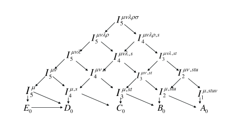
Figure 1: Graphical presentation of the tensor reduction procedure

In a few words, the idea of the reduction is that, one-loop $n$-point rank $R$ tensor Feynman integrals [in short: $(n,R)$-integrals] for $n\leq 6$ with $R\leq n$ are represented in terms of $(n,R-1)$- and $(n-1,R-1)$-integrals (see e.g. Figure 1). The recursive scheme is very convenient for explicit calculations and contains the complete calculational chain of tensor reduction, for both massive and massless propagators, and works with dimensional regularization. The general case of tensor integrals using dimensional regularization was treated in a series of papers [13, 14, 15, 16, 17], thereby allowing also for massless particles. The only necessary package to be added is one for the evaluation of 1-point to 4-point scalar integrals. These are calculated by QcdLoop [18]. This is a very interesting property of the reduction, because using Fortran and switching off the relative scalar master integrals we have all the information that is needed to determine the coefficients of the scalar master integrals that arise in calculations by unitarity methods. In the same way, by switching off all the scalar master integrals we can also extract the rational term. Finally, due to the capability of QcdLoop to give the $1/\epsilon$ and $1/\epsilon^{2}$ terms, we can cross check the correctness of our loop amplitude as these terms are proportional to the tree level amplitude.

The stripped amplitude in total is optimized by Maple. We divide the total number of diagrams to groups of hexagons, pentagons, boxes, triangles, and bubbles, and then we translate the output to Maple. Maple optimizes it and feeds it to a Fortran subroutine calculating the amplitude contributions of the above groups. As mentioned above, these structures are single colored ones. So each one of them is multiplied with the appropriate color structure stored in the color subroutine.

Connecting all the pieces together, the stripped amplitudes including tensor integrals and spinor lines separately calculated in specific subroutines, the color structures precalculated and stored in an array, we calculate the total loop amplitude. In the same way, using much simpler routines, we calculate the tree level case.

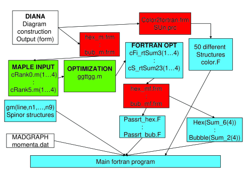
Figure 2: Graphical presentation of the case of $gg\rightarrow t\bar{t}gg$

The biggest advantage of the program is the fact that it is flexible. With minor changes, we can implement it for calculating different processes. We just have to provide Diana with the process that we are interested in, fix the Feynman rules and be careful with manipulation of possible spinor lines and colors. All the rest, tensor reduction and optimization of the code are done automatically by the program.

3 Acknowledgments

Work supported in part by Sonderforschungsbereich/Transregio SFB/TRR 9 of DFG “Computergestützte Theoretische Teilchenphysik” and by the European Community’s Marie-Curie Research Training Network MRTN-CT-2006-035505 “HEPTOOLS”. We would also like to thank our collaborators Jochem Fleischer and Tord Riemann for useful discussions.

References

- [1] A. Bredenstein, A. Denner, S. Dittmaier and S. Pozzorini, Phys. Rev. Lett. 103 (2009) 012002 [arXiv:0905.0110 [hep-ph]].
- [2] A. Bredenstein, A. Denner, S. Dittmaier and S. Pozzorini, JHEP 1003 (2010) 021 [arXiv:1001.4006 [hep-ph]].
- [3] G. Bevilacqua, M. Czakon, C. G. Papadopoulos, R. Pittau and M. Worek, JHEP 0909 (2009) 109 [arXiv:0907.4723 [hep-ph]].
- [4] C. F. Berger, Z. Bern, L. J. Dixon et al., Phys. Rev. Lett. 102 (2009) 222001. [arXiv:0902.2760 [hep-ph]].
- [5] R. Keith Ellis, K. Melnikov and G. Zanderighi, Phys. Rev. D 80 (2009) 094002 [arXiv:0906.1445 [hep-ph]]
- [6] C. F. Berger, Z. Bern, L. J. Dixon et al., Phys. Rev. D80 (2009) 074036. [arXiv:0907.1984 [hep-ph]].
- [7] C. F. Berger et al., arXiv:1004.1659 [hep-ph].
- [8] T. Binoth, N. Greiner, A. Guffanti, J. Reuter, J. P. Guillet and T. Reiter, Phys. Lett. B 685 (2010) 293 [arXiv:0910.4379 [hep-ph]].
- [9] G. Bevilacqua, M. Czakon, C. G. Papadopoulos and M. Worek, arXiv:1002.4009 [hep-ph].
- [10] M. Tentyukov and J. Fleischer, Comput. Phys. Commun. 132 (2000) 124 [arXiv:hep-ph/9904258].
- [11] J. A. M. Vermaseren, arXiv:math-ph/0010025.
- [12] T. Diakonidis, J. Fleischer, T. Riemann and J. B. Tausk, Phys. Lett. B 683 (2010) 69 [arXiv:0907.2115 [hep-ph]].
- [13] Z. Bern, L. J. Dixon and D. A. Kosower, Phys. Lett. B 302, 299 (1993) [Erratum-ibid. B 318, 649 (1993)] [arXiv:hep-ph/9212308].
- [14] Z. Bern, L. J. Dixon and D. A. Kosower, Nucl. Phys. B 412, 751 (1994) [arXiv:hep-ph/9306240].
- [15] T. Binoth, J. P. Guillet and G. Heinrich, Nucl. Phys. B 572, 361 (2000) [arXiv:hep-ph/9911342].
- [16] G. Duplancic and B. Nizic, Eur. Phys. J. C 35, 105 (2004) [arXiv:hep-ph/0303184].
- [17] T. .Diakonidis, J. Fleischer, J. Gluza et al., Phys. Rev. D80 (2009) 036003. [arXiv:0812.2134 [hep-ph]].
- [18] R. K. Ellis, G. Zanderighi, JHEP 0802 (2008) 002. [arXiv:0712.1851 [hep-ph]].