Weakly linked binary mixtures of $F=1$ ⁸⁷Rb Bose-Einstein condensates

Abstract

We present a study of binary mixtures of Bose-Einstein condensates confined in a double-well potential within the framework of the mean field Gross-Pitaevskii equation. We reexamine both the single component and the binary mixture cases for such a potential, and we investigate in which situations a simpler two-mode approach leads to an accurate description of their dynamics. We also estimate the validity of the most usual dimensionality reductions used to solve the Gross-Pitaevskii equations. To this end, we compare both the semi-analytical two-mode approaches and the numerical simulations of the 1D reductions with the full 3D numerical solutions of the Gross-Pitaevskii equation. Our analysis provides a guide to clarify the validity of several simplified models that describe mean field non-linear dynamics, using an experimentally feasible binary mixture of an $F=1$ spinor condensate with two of its Zeeman manifolds populated, $m=\pm 1$.

1 Introduction

The phase coherence of a Bose-Einstein Condensate (BEC) is an important and characteristic property of ultracold bosonic gases that leads to fascinating macroscopic phenomena such as interference effects or Josephson-type oscillations. Two condensates trapped in a double-well potential exhibit interference fringes when the barrier is released and the two expanding condensates, with a well-defined quantum phase, overlap. Instead, if the barrier is not switched-off and is large enough to ensure a weak link between both condensates in each side of the trap, the quantum phase difference will drive Josephson-like effects, which consist on fast oscillating tunneling, much faster than the single particle tunneling, of atoms through the potential barrier [1, 2].

The first evidence of the phase coherence of a BEC was obtained in early interference experiments [3] where clean interference patterns appeared in the overlapping region of two expanding condensates. It has been only recently that a clear evidence of a bosonic Josephson junction in a weakly linked scalar BEC  has been experimentally reported by the group of M. Oberthaler in Heidelberg [4]. In this experiment, two condensates are confined in a double-well potential with an initial population imbalance between both sides which triggers the Josephson oscillations. The tunneling of particles leads to a coupled dynamical evolution of the two conjugate variables, the phase difference between the two weakly linked condensates and their population imbalance. In spite of the system being very dilute, the inter-species interaction plays a crucial role in the Josephson dynamics, leading to new regimes beyond the standard Josephson effect, e.g. macroscopic quantum self trapping (MQST).

The Gross-Pitaevskii (GP) mean field theory provides a natural framework for investigating Josephson dynamics in weakly interacting systems at very low temperature. Josephson oscillations in scalar Bose-Einstein condensates have been theoretically studied by using different techniques [5, 6, 7, 8, 9, 10, 11, 12, 13, 14, 15, 16, 17, 18, 19]. As expected, the full three dimensional time-dependent Gross-Pitaevskii equation (GP3D ) provides an excellent agreement with the experimental data [9, 10, 20]. However, since 3D dynamics need in general rather involved calculations, one can benefit from the fact that the barrier is created along one direction and the tunneling of particles is mainly one dimensional (1D) to investigate the Josephson dynamics by means of effective 1D GP-like equations. Among these reduced GP equations, the non-polynomial nonlinear Schrödinger equation (NPSE ) proposed in Ref. [21] has provided the best agreement with the experimental results in scalar condensates [20], whereas another effective 1D Gross-Pitaevskii equation ( GP1D ) fail to describe the dynamics for large number of trapped atoms in the same trapping conditions as in the Heidelberg’s experiment [10, 20].

Interactions are important to understand the different regimes of the tunneling dynamics. Therefore, multi-component BECs in double-well potentials offer an interesting extension to study phenomena related to phase coherence. In particular the Josephson dynamics will become richer due to the interplay between intra- and inter-species interactions.

Josephson oscillations in binary mixtures confined in double-well potentials have been addressed in a number of recent articles. The case of two-component BECs with density-density interactions has been studied within two-mode approaches in Refs. [22, 23, 24, 25, 26, 27, 28, 29]. Refs. [26, 29] go one step further and also consider GP1D simulations. Spin-dependent interactions have been addressed in Refs. [30, 31]. Josephson dynamics in spinor condensates confined in double-wells, characterized by an exchange of population between different Zeeman components, has also been investigated in Refs. [32, 33]. In Refs. [26, 30] the interest of studying Josephson dynamics in binary mixtures has been emphasized as it can give access to information of the different scattering lengths present in the system.

Recently, the equations of the tunneling dynamics in a binary mixture within the two-mode approximation to the GP equations have been derived in Ref. [25]. However, the authors have not compared their two-mode analysis to direct numerical resolutions of the GP equation, and have also not provided microscopic values to the parameters of the two-mode equations. Their main result is the description of a symmetry breaking pattern occurring when the inter- and intra-species interactions differ substantially. In Ref. [26] a comparison of the standard two-mode approach and the coupled GP1D equations for the mixture has been presented for one specific double-well potential which allows an analytical treatment.

For single component BECs, it has been already studied the range of validity of the different approximations to the Josephson dynamics by comparing with GP3D calculations and with the experimental results. However, no comparison with the full GP3D dynamics has been yet performed for a binary mixture in a double-well potential.

The aim of this paper is to investigate systematically the tunneling dynamics of a binary mixture of BECs trapped in a double-well potential, as well as the validity of the different mean-field approximations. We consider a mixture of two components obtained by populating two Zeeman states of an $F=1$ ⁸⁷Rb condensate confined in the same double-well potential as in the experiments [4]. This system corresponds to a natural extension of the experimental work of Ref. [4], where only one of the Zeeman components was populated.

We provide a general overview of the different techniques used to investigate Josephson dynamics within the two-mode model (standard and improved two-mode) and within the Gross-Pitaevskii framework (one-dimensional reductions of the GP equation, GP1D and NPSE ). To this end, we solve the full 3D time-dependent GP equation for the mixture as a reference to assess and analyze the validity of the previous approximations.

The paper is organized as follows. The general framework of the coupled Gross-Pitaevskii equations for a binary mixture is presented in Sec. 2. In Sec. 3, we derive analytic two-mode models both for single and two component systems. First we recall the standard two-mode model (S2M ). Then we derive the equations of the improved two-mode model (I2M ) for a binary mixture, generalizing the work for a single component BEC performed in Ref. [9]. We discuss the stability of the dynamical equations and look for the stationary points for a binary mixture. In Sec. 4, we analyze the different one-dimensional reductions of the GP3D equations for the mixture: GP1D and NPSE . In Sec. 5, we revisit the dynamics of a single component condensate in a double-well potential with the same parameters as in the experiment [4]. The tunneling dynamics in two-component systems is accurately discussed in Sec. 6. We obtain the dynamics by solving the coupled GP3D equations for the mixture and show that for certain conditions there exists a good agreement between I2M and GP3D , as well as for NPSE and GP3D . The range of validity of the two-mode models is explored, paying special attention to situations which fall beyond the two-mode approximation. Finally, we discuss cases that present characteristic features arising from the mixture, with no analog in the tunneling dynamics of a single component BEC. Conclusions are given in Sec. 7.

2 Mean field approach: Gross-Pitaevskii equations

We consider a binary mixture of weakly interacting atoms at zero temperature, confined by the same double-well potential, $V({\bf r})$. For dilute systems with sufficiently large number of particles, the Gross-Pitaevskii equation provides a suitable framework to study the dynamics. In the mean field approximation, each condensate is described by the corresponding wave function $\Psi_{i}({\bf r};t)$, with $i=a,b$ denoting each of the two components of the binary mixture. To avoid any misunderstanding let us remind the reader that we are describing two different kind of atoms, $a$ and $b$, which evolve on a double-well external potential. In most situations, the system will behave as if there were four weakly linked Bose-Einstein condensates, two per each component of the binary mixture per each side of the potential barrier. The mean field description will reflect this feature by the homogeneous quantum phase of $\Psi_{i}({\bf r};t)$ at each side of the potential barrier, as will be discussed in great detail in the following sections.

The dynamical evolution of the two wave functions can be obtained by solving the two coupled GP equations:

$$i\hbar{\partial\Psi_{a}({\bf r};t)\over\partial t} = \left[-{\hbar^{2}\over 2m_{a}}\nabla^{2}+V({\bf r})+g_{aa}N_{a}|\Psi_{a}({\bf r};t)|^{2}+g_{ab}N_{b}|\Psi_{b}({\bf r};t)|^{2}\right]\Psi_{a}({\bf r};t)$$

$$i\hbar{\partial\Psi_{b}({\bf r};t)\over\partial t} = \left[-{\hbar^{2}\over 2m_{b}}\nabla^{2}+V({\bf r})+g_{ba}N_{a}|\Psi_{a}({\bf r};t)|^{2}+g_{bb}N_{b}|\Psi_{b}({\bf r};t)|^{2}\right]\Psi_{b}({\bf r};t)\,.$$

For each component, the condensate wave function $\Psi_{i}({\bf r};t)$ is normalized to 1, $m_{i}$ is the atomic mass, and $g_{ii}=4\pi\hbar^{2}a_{i}/m_{i}$ is the effective atomic interaction between atoms of the same species, with $a_{i}$ the corresponding $s$-wave scattering length. The coupling between both components is governed by the inter-species interaction $g_{ab}\equiv g_{ba}$, which depends on the specific nature of the binary mixture. The total number of atoms in the mixture is $N=N_{a}+N_{b}$.

There are many experimental possibilities to study the dynamics of binary mixtures of BECs. We will restrict our study to one of them, which is experimentally feasible. We will consider binary mixtures made of $F=1$ ⁸⁷Rb atoms populating the $m=\pm 1$ Zeeman sublevels [34]. This implementation greatly simplifies the dynamics as the inter- and intra-species couplings are very similar in magnitude. Of course this choice limits the phenomena which can be observed, e.g. the interesting symmetry breaking pattern discussed in Ref. [25], which relies on the inter-species coupling being larger than the intra-species one, will not take place, see Sec. 6.5.

On the other hand its simplicity allows to discuss in detail the different approaches taken in the literature, e.g. two-mode models of the GP equations, one dimensional reductions, etc. As occurred in the scalar case, the dynamical features contained in Eqs. (LABEL:GP-mixture) can to a large extent be described by a simplified two-mode model for each component. In the next section we follow Refs. [5], [9] and [25] and derive two-mode expressions for the scalar and binary case. The usual assumption of neglecting the overlaps involving the right and left modes gives rise to the so called standard two-mode (S2M ) equations, while retaining them one also gets a closed system of equations, the improved two-mode (I2M ). Both the S2M and I2M are also derived for the binary mixture case.

3 Two-mode approaches

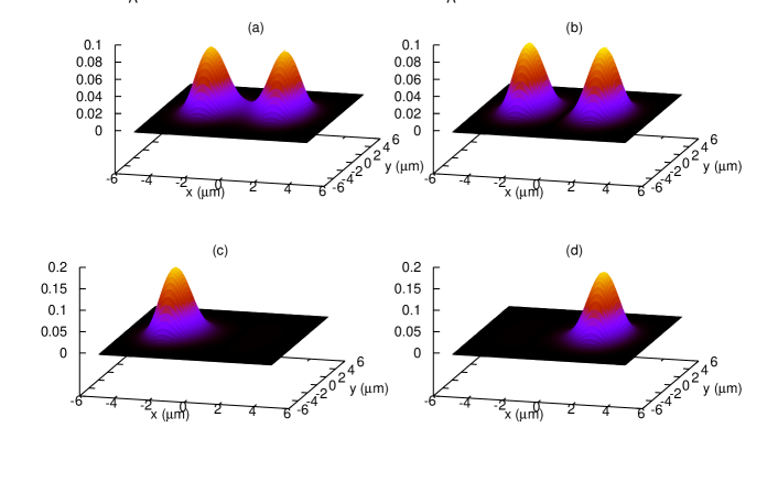
Figure 1: 3D depictions of the density, $\rho(x,y)=\int dz|\Psi(x,y,z)|^{2}$ in $(\mu m)^{-2}$, of the $(a)$ ground state, $(b)$ first excited state, $(c)$ left mode and $(d)$ right mode obtained by performing an imaginary time GP3D calculation with the same conditions as in the experimental setup of Ref. [4].

The two-mode approximation allows to study the dynamics of weakly linked Bose-Einstein condensates, without solving the full GP3D nor reducing the dimensionality of the GP equation [5, 9]. Depending on the specific double-well potential, e.g. on the energy gap between the first two levels of the single particle Hamiltonian and the next two, it can provide an excellent description of the full GP solution. The relevant physical quantity is the ratio between the energy gap between the ground state and first excited state of the double-well potential, $\delta E_{0;1}=E_{1}-E_{0}$  and the energy difference of the ground state and the second excited state, $\delta E_{0;2}=E_{2}-E_{0}$. The smaller the ratio $\delta E_{0;1}/\delta E_{0;2}$ the more accurate the two-mode approach. The two mode description characterizes the dynamics of the scalar condensate in a double-well potential with only two variables: the relative population and the phase difference between the left and right side of the potential barrier.

3.1 Standard two-mode model for the single component case

The GP equation for the scalar case corresponds to a particular limit of the GP equations for the binary mixture, Eqs. (LABEL:GP-mixture),

$$i\hbar{\partial\Psi({\bf r};t)\over\partial t}=\left[-{\hbar^{2}\over 2m}\nabla^{2}+V({\bf r})+gN|\Psi({\bf r};t)|^{2}\right]\Psi({\bf r};t)\,.$$ (2)

We will make use of the following notation, $H_{0}=-(\hbar^{2}/2m)\nabla^{2}+V({\bf r})$, and $H_{g}[\Psi]=gN|\Psi({\bf r};t)|^{2}$. Let us recall the two-mode approximation for a single component condensate in a double-well potential. We consider $N$ interacting atoms with atomic mass $m$, and coupling constant $g$, trapped in a symmetric double-well potential $V({\bf r})$. When both sides of the potential barrier are weakly linked, the total wave function can be approximately written as a superposition of two time-independent spatial wave functions $\Phi_{L(R)}({\bf r})$ mostly localized at the left (right) side of the trap:

$$\Psi({\bf r};t)=\Psi_{L}(t)\Phi_{L}({\bf r})+\Psi_{R}(t)\Phi_{R}({\bf r})\,.$$ (3)

The left and right modes, can be expressed as linear combinations of the ground (+) and the first excited ($-$) states of the double-well potential including the interaction term. They satisfy, $(H_{0}+H_{g}[\Phi_{\pm}])\Phi_{\pm}=\mu_{\pm}\Phi_{\pm}$, and the left/right modes can be written as [9]:

$$\Phi_{L}({\bf r}) = \frac{\Phi_{+}({\bf r})+\Phi_{-}({\bf r})}{\sqrt{2}}\;,\qquad\Phi_{R}({\bf r})=\frac{\Phi_{+}({\bf r})-\Phi_{-}({\bf r})}{\sqrt{2}}\,\,.$$ (4)

We observe that in a symmetric double-well, $\Phi_{\pm}$ have a well defined parity: $\Phi_{\pm}({\bf r})=\pm\Phi_{\pm}(-{\bf r})\,,$ and therefore $\langle\Phi_{i}\Phi_{j}\rangle=\delta_{ij}$ with $i,j=+,-$. Since they are stationary solutions of the GP equation, $\Phi_{\pm}$ are real functions, and so are the left and right modes $\Phi_{L(R)}$. The integrated density in the z-direction, $\rho(x,y)=\int dz|\Psi(x,y,z)|^{2}$, associated to the ground ($\Phi_{+}$), and first excited ($\Phi_{-}$) states are depicted in Fig. 1 together with the densities associated to the left and right modes. The plots correspond to the experimental set up of Ref. [4].

From the phase coherence properties of a BEC, one can assume that the wave function in each side of the trap has a well defined quantum phase $\phi_{j}(t)$, which is independent of the position but changes during the time evolution. We can write,

$$\Psi_{j}(t)=\sqrt{N_{j}(t)}e^{i\phi_{j}(t)}\,,$$ (5)

where $N_{L(R)}(t)$ corresponds to the number of atoms on the left (right) side of the trap, and the total number of atoms is $N=N_{L}(t)+N_{R}(t)$. The weak link condition is fulfilled if $(\mu_{-}-\mu_{+})<<(1/2)(\mu_{+}+\mu_{-})$.

As a first step, we consider the so-called standard two-mode approximation (S2M ), which neglects a certain set of overlapping integrals involving mixed products of $\Phi_{L}$ and $\Phi_{R}$. This approximation yields essentially the correct qualitative results in the scalar condensate although it may lead to incorrect quantitative predictions depending on the specific barrier properties [4, 9] .

Inserting the two-mode ansatz (3) in the GP equation for a single component condensate (2) and neglecting terms involving mixed products of $\Phi_{L}$ and $\Phi_{R}$ of order larger than one, yields into a system of equations for the two localized modes which can be written in terms of two dynamical variables: the population imbalance $z(t)=[N_{L}(t)-N_{R}(t)]/N$ and the phase difference $\delta\phi(t)=\phi_{R}(t)-\phi_{L}(t)$ between each side of the barrier:

$$\dot{z}(t) = -\omega_{R}\sqrt{1-z^{2}(t)}\,\sin{\delta\phi(t)}$$ (6)

$$\dot{\delta\phi(t)} = \omega_{R}\,\Delta E+\omega_{R}{U_{L}+U_{R}\over 4K}Nz(t)+\omega_{R}{z(t)\over\sqrt{1-z^{2}(t)}}\,\cos{\delta\phi(t)}\,,$$

where $\omega_{R}=2K/\hbar$ is the Rabi frequency and

$$\Delta E = {E_{L}^{0}-E_{R}^{0}\over 2K}+{U_{L}-U_{R}\over 4K}N$$

$$E^{0}_{L(R)} = \int d{\bf r}\bigg{[}{\hbar^{2}\over 2m}\,\big{|}\nabla\Phi_{L(R)}({\bf r})\big{|}^{2}+\Phi_{L(R)}^{2}({\bf r})\,V({\bf r})\bigg{]}$$

$$K = -\int d{\bf r}\bigg{[}{\hbar^{2}\over 2m}\,\nabla\Phi_{L}({\bf r})\cdot\nabla\Phi_{R}({\bf r})+\Phi_{L}({\bf r})\,V({\bf r})\,\Phi_{R}({\bf r})\bigg{]}$$

$$U_{L(R)} = g\int\!d{\bf r}\,\Phi_{L(R)}^{4}({\bf r})\;.$$ (7)

For a symmetric double-well, $E_{L}^{0}=E_{R}^{0}$ and $U_{L}=U_{R}\equiv U$, therefore $\Delta E=0$. Moreover, the Rabi frequency only appears as a scale in the problem and thus can be absorbed in the time by rescaling $t\to\omega_{R}t$. Then, together with the definition $\Lambda\equiv NU/(\hbar\omega_{R})$, we obtain,

$$\dot{z}(t) = -\sqrt{1-z^{2}(t)}\,\sin{\delta\phi(t)}$$ (8)

$$\dot{\delta\phi(t)} = {\Lambda z(t)}+{z(t)\over\sqrt{1-z^{2}(t)}}\,\cos{\delta\phi(t)}\,.$$

Note that, $\Lambda>0$ and $\Lambda<0$ correspond to repulsive and attractive atom-atom interactions, respectively. There are different regimes depending on the initial values of the population imbalance and phase difference, $z(0)$ and $\delta\phi(0)$, Sec. 3.3.

From the energy functional of the GP equation (2):

$$E[\Psi({\bf r};t)]=\int d{\bf r}\bigg{[}{\hbar^{2}\over 2m}\Big{|}\vec{\nabla}\Psi({\bf r};t)\Big{|}^{2}+V({\bf r})\big{|}\Psi({\bf r};t)\big{|}^{2}+{g\over 2}\big{|}\Psi({\bf r};t)\big{|}^{4}\bigg{]}$$ (9)

and using the two-mode ansatz (3), we can define the conserved energy per particle of the system as:

$$H\equiv{E[\Psi({\bf r};t)]-C\over NK}=\Delta E\,z(t)+{U_{L}+U_{R}\over 8K}Nz^{2}(t)-\sqrt{1-z^{2}(t)}\cos{\delta\phi(t)}$$

where $C$ is a rescaling constant. If we consider again a symmetric double-well we have:

$$H={\Lambda\over 2}z^{2}(t)-\sqrt{1-z^{2}(t)}\cos{\delta\phi(t)}\;.$$ (11)

Note that the equations of motion (8) can be written in the Hamiltonian form:

$$\dot{z}=-{\partial H\over\partial\delta\phi}\;;\qquad\delta\dot{\phi}={\partial H\over\partial z}$$ (12)

being $z$ and $\delta\phi$ canonical conjugate variables.

3.2 Improved two-mode model for the single component case

Ananikian and Bergeman [9] noticed that for a symmetric double-well there was no need to neglect any of the overlapping integrals to obtain a closed set of equations relating $z$ and $\delta\phi$.

Thus, remaining in the two-mode approximation but retaining all the overlaps it is straightforward to write down the following set of equations (cf. Eqs. (22) in Ref. [9]), called the “improved two-mode” (I2M ) equations,

$$\dot{z}(t) = -B\sqrt{1-z^{2}(t)}\,\sin{\delta\phi}(t)+C(1-z^{2}(t))\sin 2\delta\phi(t)$$ (13)

$$\dot{\delta\phi(t)} = {Az(t)}+{Bz(t)\over\sqrt{1-z^{2}(t)}}\,\cos{\delta\phi}(t)-Cz(t)\cos 2\delta\phi(t)\,.$$

Defining, $\gamma_{ij}=g\int\!d{\bf r}\,\Phi_{i}^{2}({\bf r})\Phi_{j}^{2}({\bf r})\;,i,j=+,-$, we have, $A=N\left(10\gamma_{+-}-\gamma_{++}-\gamma_{--}\right)/4$, $B=2K+N(\gamma_{--}-\gamma_{++})/2$, and $C=gN\int\!d{\bf r}\,\Phi_{L}^{2}({\bf r})\Phi_{R}^{2}({\bf r})$.

As discussed in detail in Ref. [9], the physics arising from the I2M is similar to the one present in the S2M . The I2M , however, is in much better agreement with the GP3D for a broader set of double-well potentials, as we will see in Sec. 5. In particular, for the double-well considered in the experimental setup of the Heidelberg group [4] the S2M (with the corresponding microscopic parameters, $K$ and $U$, computed from the GP3D with the experimental 3D potential and experimental coupling, $g$) does not correctly predict the physics of the experiment, mainly due to the importance of the neglected overlaps, and not to a dynamics far from a two-mode one.

3.3 Regimes for the single component case

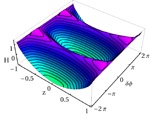
Figure 2: Energy surface, Eq.(11), for $\Lambda=2.5$. The lines on the surface correspond to possible trajectories of the system.

3.3.1 Stability analysis

In this section we use the S2M to analyze the stability of the single component system, and focus on the case of repulsive interactions $\Lambda>0$. Using the Hamiltonian (11) and the equations of motion (12), the stationary points ($z^{0}$, $\delta\phi^{0}$) can be found by solving the equations:

$$\left.{\partial H\over\partial z}\right|_{z^{0},\delta\phi^{0}}=0\;;\qquad\left.{\partial H\over\partial\delta\phi}\right|_{z^{0},\delta\phi^{0}}=0\,.$$ (14)

To asses the stability of these points, we need to study the Hessian matrix of the system, which for the possible values of the phase difference, $\delta\phi^{0}=0$ or $\pi$, is always diagonal and its eigenvalues are $\partial^{2}_{z}H|_{z^{0},\delta\phi^{0}}$ and $\partial^{2}_{\delta\phi}H|_{z^{0},\delta\phi^{0}}$. Depending on the sign of these eigenvalues the stationary points will be maxima, saddle points or minima. The stationary points and their stability are summarized in Table 1.

($z^{0}$, $\delta\phi^{0}$)	stationary	minimum	saddle	maximum
($0$, $0$)	$\forall\Lambda$	$\forall\Lambda$	—	—
($0$, $\pi$)	$\forall\Lambda$	—	$\Lambda>1$	$\Lambda<1$
($\pm\sqrt{1-1/\Lambda^{2}}$, $\pi$)	$\Lambda>1$	—	—	$\Lambda>1$

Table 1: Stationary points of the system for repulsive interactions, $\Lambda>0$, and their stability.

The evolution of the system can be represented on a $z-\delta\phi$ plane, where the system follows trajectories with constant energy, $H$, see curves in Fig. 2. Note that oscillations around a stationary point, closed curves, occur only if the central point is either a maximum or a minimum of the energy, but not a saddle point. As we will see in the following sections, these orbits will give rise to the Josephson oscillations and to the zero- and $\pi$-modes.

3.3.2 Symmetry between attractive and repulsive interactions

$z(0)$

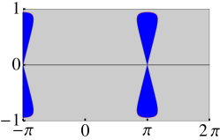
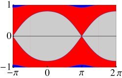
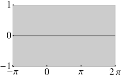
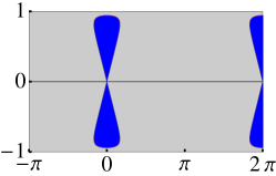
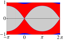
$\delta\phi(0)$

Figure 3: Different regimes for a set of initial conditions, imbalance $z(0)$ in the y-axis and phase difference $\delta\phi(0)$ in the x-axis. The upper panels correspond to repulsive interactions while the lower ones to attractive interactions. The values of $|\Lambda|$ are 0.5, 1.5, and 5. for the left, middle and right panels respectively. Grey regions correspond to Josephson oscillations, blue regions to $\pi$-modes (upper panels) and zero-modes (lower panels), and red regions to running phase modes.

The stability analysis has been presented only for repulsive interactions, but from the system (8) we can see that if we change the interactions, $\Lambda\longrightarrow-\Lambda$, we recover the same system of equations if $\delta\phi\longrightarrow\pi-\delta\phi$:

$${d\over dt}z(t) = -\sqrt{1-z^{2}(t)}\,\sin{(\pi-\delta\phi(t))}$$ (15)

$${d\over dt}(\pi-\delta\phi(t)) = -\Lambda z(t)-{z(t)\over\sqrt{1-z^{2}(t)}}\,\cos({\pi-\delta\phi(t)})\,,$$

which means that the dynamics of the system and the different regimes are the same for both interactions, with a phase-shift of $\pi$. This can be seen in Fig. 3, that shows the behavior of the system for a given set of initial conditions. The upper panels are for repulsive interactions $\Lambda>0$ and the lower ones for attractive interactions $\Lambda<0$. The grey regions correspond to Josephson oscillations, the blue regions to zero- and $\pi$-modes, and the red regions to running phase modes, as it will be seen in the following sections.

3.3.3 Josephson dynamics

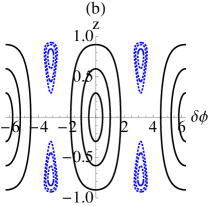
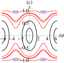
Figure 4: $z-\phi$ representation of different constant energy trajectories for three values of $\Lambda$: 0.5 (a), 1.5 (b), and 5 (c). Solid-black lines correspond to Josephson oscillations, dotted-blue to $\pi$-modes, and dashed-red lines to running phase modes.

This regime is characterized by fast oscillating tunneling of population across the potential barrier. Plotted in a $z-\delta\phi$ map, the system evolves following closed trajectories around a minimum or a maximum ($z^{0}=0,\delta\phi^{0}$) configuration, with a zero time-average of the population imbalance, $<z>_{t}=0$. The stability analysis shows that for $\Lambda>-1$, which corresponds to repulsive or slightly attractive interactions, the stationary point $(z^{0}=0,\delta\phi^{0}=0$) is a minimum permitting Josephson oscillations around it. Analogously, for $\Lambda<1$, either attractive or slightly repulsive interactions, the stationary point ($z^{0}=0$, $\delta\phi^{0}=\pi$) becomes a maximum, and therefore also allows for closed orbits around it. For $|\Lambda|>1$, there are Josephson oscillations around only one point: ($z^{0}=0$, $\delta\phi^{0}=0$), or ($z^{0}=0$, $\delta\phi^{0}=\pi$). However, in the region of weak interaction, $|\Lambda|<1$, the oscillations around both points are allowed.

In panel (a) of Fig. 4, $\Lambda=0.5$, the black closed orbits around $\delta\phi^{0}=0$ or around $\delta\phi^{0}=\pi$ correspond to Josephson dynamics around these points. In panel (b) however, as $\Lambda=1.5>1$, only the origin can give rise to Josephson oscillations, so the closed orbits around $(z^{0}=0,\delta\phi^{0}=\pi)$ disappear.

It is also interesting to study the behavior of the system for small oscillations around these two stationary points of zero imbalance, smallest orbits in Fig. 4 (a). In this limit, the system (8) can be linearized giving the dynamical equation: $\ddot{z}(t)=-z(t)(1+\Lambda\cos{\delta\phi^{0}})$ with $\cos{\delta\phi^{0}=\pm 1}$. The population imbalance performs sinusoidal oscillations with a frequency $\omega_{J}=\omega_{R}\sqrt{1+\Lambda\cos{\delta\phi^{0}}}$, independent of the initial conditions. Note that this frequency only exists when these points are either maxima or minima. The phase difference oscillates with the same frequency but with a phase-shift of $\pi/2$ with respect to the imbalance. If the initial population imbalance increases, the dynamics of the system changes substantially to non-sinusoidal oscillations, and the frequency becomes dependent on the initial conditions.

3.3.4 Macroscopic quantum self trapping

In the case of repulsive interactions, we have seen that for $\Lambda>1$, the stationary point ($z^{0}=0$, $\delta\phi^{0}=\pi$) becomes a saddle point and there appear two maxima, ($z^{0}=\pm\sqrt{1-1/\Lambda^{2}}$, $\delta\phi^{0}=\pi$). A similar behavior is found for attractive interactions. These stationary points allow for oscillations around them with $<z>_{t}\neq 0$. In fact, in this regime, the imbalance has the same sign during the evolution, and therefore one of the wells is always overpopulated.

This regime is called macroscopic quantum self trapping, as the tunneling is strongly suppressed and the particles remain mostly trapped in one of the wells. This is a phenomenon arising from the atom-atom interaction, which appears as a non-linearity in the Gross-Pitaevskii equation.

The critical condition for the existence of the MQST regime can be found by imposing that the system remains on one side of the trap  [5]. For a given set of initial conditions, $z(0)\neq 0$ and $\delta\phi(0)$, the system will remain trapped if,

$$\Lambda > 2\left({\sqrt{1-z(0)^{2}}\cos[\delta\phi(0)]+1\over z(0)^{2}}\right)\qquad{\rm for\;}\Lambda>1$$

$$\Lambda < 2\left({\sqrt{1-z(0)^{2}}\cos[\delta\phi(0)]-1\over z(0)^{2}}\right)\qquad{\rm for\;}\Lambda<-1\,,$$ (16)

where the limits of the interaction parameter are due to the fact that only when $|\Lambda|>1$ the $(z^{0}\neq 0,\delta\phi^{0})$ stationary points exist.

In this regime however, there are two different kind of MQST depending on whether the phase difference evolves bounded, giving the so-called zero- and $\pi$-modes, or whether it evolves unbounded, increasing (or decreasing) always in time, giving rise to the running phase modes.

For values of the interaction parameter of $1<|\Lambda|<2$ the only MQST regime that one can have is the zero-mode for attractive interactions and the $\pi$-mode for repulsive interactions (which are plotted in blue dotted lines in panel (b) of Fig. 4). In these regimes the phase difference evolves bounded around $\delta\phi=0$ and $\delta\phi=\pi$, respectively.

On the other hand, for values of $|\Lambda|>2$ one can have both classes of MQST. In general however, for a given set of initial conditions, the system will evolve following a running phase mode (dashed-red lines of panel (c) of Fig. 4), because the values of $z^{0}=\pm\sqrt{1-1/\Lambda^{2}}$, that allow closed orbits, are very close to 1 (see the small $\pi$-modes of panel (c) in blue dotted lines).

In panel (c), one can see that the broadest closed orbit around ($z^{0}\neq 0$, $\delta\phi^{0}=\pi$), for $\Lambda>2$, is the one that goes through ($z=\pm 1$, $\delta\phi=0$). Notice that an orbit that crosses the $\delta\phi=0$ axis in any other point, $z\neq\pm 1$, would correspond to a running phase mode. The case of attractive interactions can be understood by taking into account the phase-shift of $\pi$ in $\delta\phi$. The latter can be used to find the condition to have bounded or running phase difference modes. For a given set of initial conditions ($z(0)$, $\delta\phi(0)$) fulfilling the self-trapping condition (16), the system will evolve in a bounded phase mode only if:

$$|\Lambda|<{2\cos{\delta\phi(0)}\over\sqrt{1-z^{2}(0)}}\;.$$ (17)

Moreover, in a zero- or a $\pi$-mode MQST, we can study small oscillations around the corresponding minima or maxima, $z(t)=z^{0}+\delta z$ and $\delta\phi(t)=\delta\phi^{0}+\hat{\delta\phi}(t)$, so the linearized system (8) becomes:

$$\delta\ddot{z}(t)=-\delta z(t)\left[1+\Lambda\cos{\delta\phi^{0}}{1-2(z^{0})^{2}\over\sqrt{1-(z^{0})^{2}}}\right]$$ (18)

which gives a sinusoidal behavior with a frequency:

$$\omega=\omega_{R}\sqrt{1+\Lambda\cos{\delta\phi^{0}}{1-2(z^{0})^{2}\over\sqrt{1-(z^{0})^{2}}}}\;.$$ (19)

3.4 Standard two-mode model for the binary mixture

Let us recall the two-mode approximation for weakly linked binary mixtures [22, 23, 24, 25]. The total wave function of each component is written as a superposition of two time-independent spatial wave functions localized in each well:

$$\Psi_{j}({\bf r};t)=\Psi_{jL}(t)\Phi_{jL}({\bf r})+\Psi_{jR}(t)\Phi_{jR}({\bf r})\,,$$ (20)

with $\langle\Phi_{i\alpha}|\Phi_{j\beta}\rangle=\delta_{ij}\delta_{\alpha\beta}$, $i,j=a,b$ and $\alpha,\beta=L,R$. For a given component, the condensates in each side of the trap are weakly linked. Then, as in the scalar case, one can assume that the wave function in each side of the trap has a well defined quantum phase $\phi_{j,\alpha}(t)$, which is independent of the position but which changes during the time evolution. Thus,

$$\Psi_{j,\alpha}(t)=\sqrt{N_{j,\alpha}(t)}e^{i\phi_{j,\alpha}(t)}\,.$$ (21)

$N_{j,L(R)}(t)$ corresponds to the population of the $j$-component on the left (right) side of the trap, with $N_{j}=N_{j,L}(t)+N_{j,R}(t)$. Inserting the two-mode ansatz (20) in the coupled GP equations for the mixture (LABEL:GP-mixture), retaining up to first order crossed terms yields the following system of coupled equations:

$$\dot{z_{a}}(t) = -{2K_{a}\over\hbar}\sqrt{1-z_{a}^{2}(t)}\sin{\delta\phi_{a}(t)}$$

$$\dot{\delta\phi_{a}}(t) = \Delta E_{a,b}+{U_{aaL}+U_{aaR}\over 2\hbar}N_{a}z_{a}(t)+{U_{abL}+U_{abR}\over 2\hbar}N_{b}z_{b}(t)$$

$$+{2K_{a}\over\hbar}{z_{a}(t)\over\sqrt{1-z_{a}^{2}(t)}}\cos{\delta\phi_{a}(t)}$$

$$\dot{z_{b}}(t) = -{2K_{b}\over\hbar}\sqrt{1-z_{b}^{2}(t)}\sin{\delta\phi_{b}(t)}$$

$$\dot{\delta\phi_{b}}(t) = \Delta E_{b,a}+{U_{bbL}+U_{bbR}\over 2\hbar}N_{b}z_{b}(t)+{U_{baL}+U_{baR}\over 2\hbar}N_{a}z_{a}(t)$$ (22)

$$+{2K_{b}\over\hbar}{z_{b}(t)\over\sqrt{1-z_{b}^{2}(t)}}\cos{\delta\phi_{b}(t)}\,.$$

where,

$$\Delta E_{i,j} = {E_{iL}^{0}-E_{iR}^{0}\over\hbar}+{U_{iiL}-U_{iiR}\over 2\hbar}N_{i}+{U_{ijL}-U_{ijR}\over 2\hbar}N_{j}$$

$$E_{j\alpha}^{0} = \int d{\bf r}\;\bigg{[}{\hbar^{2}\over 2m_{j}}|\nabla\Phi_{j\alpha}({\bf r})|^{2}+\Phi_{j\alpha}^{2}V({\bf r})\bigg{]}$$

$$K_{j} = -\int d{\bf r}\;\bigg{[}{\hbar^{2}\over 2m_{j}}\,\nabla\Phi_{jL}({\bf r})\cdot\nabla\Phi_{jR}({\bf r})+\Phi_{jL}({\bf r})\,V({\bf r})\,\Phi_{jR}({\bf r})\bigg{]}$$

$$U_{ij\alpha} = g_{ij}\int d{\bf r}\;\Phi_{i\alpha}^{2}({\bf r})\Phi_{j\alpha}^{2}({\bf r})$$ (23)

with $i,j=a,b\;{\rm and}\;\alpha=L,R$. Let us consider a mixture with the same atomic mass for both components $M\equiv m_{a}=m_{b}$, which are trapped in the same symmetric double-well potential. Then, the localized modes are the same for both components but depend on the site: $\Phi_{L(R)}\equiv\Phi_{a,L(R)}=\Phi_{b,L(R)}$. Therefore, $E_{aL}^{0}=E_{bL}^{0}=E_{aR}^{0}=E_{bR}^{0}\equiv E$, $U_{aaL}=U_{bbL}=U_{aaR}=U_{bbR}\equiv U$ and $U_{abL}=U_{baL}=U_{abR}=U_{baR}\equiv\tilde{U}$, $K_{a}=K_{b}\equiv K$. Defining for each component the population imbalance and phase difference between both sides of the barrier,

$$z_{j}(t)=(N_{j,L}(t)-N_{j,R}(t))/N_{j}\,,\qquad\delta\phi_{j}(t)=\phi_{j,R}(t)-\phi_{j,L}(t)$$ (24)

the above equations can be rewritten as:

$$\dot{z_{a}}(t) = -\omega_{R}\sqrt{1-z_{a}^{2}(t)}\,\sin{\delta\phi_{a}(t)}$$ (25)

$$\dot{\delta\phi_{a}}(t) = {N_{a}Uz_{a}(t)+N_{b}\tilde{U}z_{b}(t)\over\hbar}+\omega_{R}{z_{a}(t)\over\sqrt{1-z_{a}^{2}(t)}}\,\cos{\delta\phi_{a}}(t)$$

$$\dot{z_{b}}(t) = -\omega_{R}\sqrt{1-z_{b}^{2}(t)}\,\sin{\delta\phi_{b}}(t)$$

$$\dot{\delta\phi_{b}}(t) = {N_{b}Uz_{b}(t)+N_{a}\tilde{U}z_{a}(t)\over\hbar}+\omega_{R}{z_{b}(t)\over\sqrt{1-z_{b}^{2}(t)}}\,\cos{\delta\phi_{b}}(t)\,,$$

where $\omega_{R}=2K/\hbar$ is the Rabi frequency, the same for both species. It is useful to define, $\Lambda=NU/\hbar\omega_{R}$, $\tilde{\Lambda}=N\tilde{U}/\hbar\omega_{R}$, $f_{a}=N_{a}/N$, $f_{b}=N_{b}/N$ and rescale the time as $t\to\omega_{R}t$,

$$\dot{z_{a}}(t) = -\sqrt{1-z_{a}^{2}(t)}\,\sin{\delta\phi_{a}}(t)$$ (26)

$$\dot{\delta\phi_{a}}(t) = {f_{a}\Lambda z_{a}(t)+f_{b}\tilde{\Lambda}z_{b}(t)}+{z_{a}(t)\over\sqrt{1-z_{a}^{2}(t)}}\,\cos{\delta\phi_{a}}(t)$$

$$\dot{z_{b}}(t) = -\sqrt{1-z_{b}^{2}(t)}\,\sin{\delta\phi_{b}}(t)$$

$$\dot{\delta\phi_{b}}(t) = {f_{b}\Lambda z_{b}(t)+f_{a}\tilde{\Lambda}z_{a}(t)}+{z_{b}(t)\over\sqrt{1-z_{b}^{2}(t)}}\,\cos{\delta\phi_{b}}(t)\,.$$

These equations correspond to two coupled nonrigid pendulums. The stability of these systems of equations have been analyzed recently in Ref. [24].

3.5 Improved two-mode model for the binary mixture

As was noted for the scalar case in Ref. [9], it is not mandatory to neglect any of the overlaps to obtain a closed set of equations relating the population imbalances and phase differences for a symmetric double-well potential. The complete set of two-mode equations were called the improved two-mode (I2M ) equations.

In principle, if the experimental setup is appropriately chosen the left and right modes may be quite well localized at each side of the trap. In this case, the S2M equations are expected to provide quantitative agreement with the experimental data. When the two-modes are not so well localized, then it becomes necessary to consider the I2M to have quantitative agreement. In [9] the authors considered explicitly the set up of the Heidelberg group and showed that the I2M is necessary in the single component case to provide a quantitative understanding of the experimental data.

Following similar steps as in the previous section and assuming the double-well potential to be symmetric as in the experiment, then the wave functions for the ground state and first excited state, $\Phi_{j\pm}({\bf r})$, have a well defined parity. The symmetry properties and the ortho-normalization conditions are capital to derive the coupled equations within the I2M model: $\Phi_{j\pm}({\bf r})=\pm\Phi_{j\pm}(-{\bf r})$ , $\langle\Phi_{i\alpha}|\Phi_{j\beta}\rangle=\delta_{ij}\,\delta_{\alpha\beta}\,,\,{\rm for\;}i,j=a,b\,\,\,{\rm and}\,\,\,\alpha,\beta=+,-\,.$ The I2M provides an exact description of the dynamics in the symmetric double-well potential, with no approximations beyond the assumption of a two-mode ansatz of the total wave function $\Psi_{j}({\bf r};t)$, Eq. (20).

The resulting system of equations relating the population imbalance and phase difference for each component within the I2M approximation reads:

$$\dot{z}_{a}(t) = -{2K_{ab}\over\hbar}\sqrt{1-z_{a}^{2}(t)}\sin{\delta\phi_{a}}(t)$$

$$\dot{\delta\phi}_{a}(t) = {\Delta_{a}(t)\over\hbar}+{2K_{ab}(t)\over\hbar}{z_{a}(t)\over\sqrt{1-z_{a}^{2}(t)}}\cos{\delta\phi_{a}}(t)$$

$$\dot{z}_{b}(t) = -{2K_{ba}(t)\over\hbar}\sqrt{1-z_{b}^{2}(t)}\sin{\delta\phi_{b}}(t)$$

$$\dot{\delta\phi}_{b}(t) = {\Delta_{b}(t)\over\hbar}+{2K_{ba}(t)\over\hbar}{z_{b}(t)\over\sqrt{1-z_{b}^{2}(t)}}\cos{\delta\phi_{b}}(t)$$ (27)

with

$$\Delta_{a}(t) = 2\,\gamma_{+-}^{aa}N_{a}\,z_{a}(t)+2\,\gamma_{+-+-}^{aabb}\,N_{b}z_{b}(t)\,,$$

$$\Delta_{b}(t) = 2\,\gamma_{+-}^{bb}\,N_{b}z_{b}(t)+2\,\gamma_{+-+-}^{bbaa}\,N_{a}z_{a}(t)\,\,,$$ (28)

where we have defined

$$\gamma_{\alpha\beta}^{ij} = g_{ij}\;\int d{\bf r}\,\Phi_{i\alpha}^{2}({\bf r})\Phi_{j\beta}^{2}({\bf r})$$ (29)

$$\gamma_{+-+-}^{aabb} = \gamma_{+-+-}^{bbaa}=g_{ab}\;\int d{\bf r}\,\Phi_{a+}({\bf r})\Phi_{a-}({\bf r})\Phi_{b+}({\bf r})\Phi_{b-}({\bf r})\,,$$

and

$$2K_{ab}(t) = (\mu_{-}^{a}-\mu_{+}^{a})+{1\over 2}\Bigg{[}N_{a}\left(\gamma_{++}^{aa}-\gamma_{--}^{aa}\right)$$

$$+ N_{b}\left(\gamma_{++}^{ab}-\gamma_{--}^{ab}-\gamma_{+-}^{ab}+\gamma_{-+}^{ab}\right)$$

$$- N_{a}\Big{(}\gamma_{++}^{aa}+\gamma_{--}^{aa}-2\gamma_{+-}^{aa}\Big{)}\sqrt{1-z_{a}^{2}(t)}\cos{\delta\phi_{a}}(t)$$

$$- N_{b}\Big{(}\gamma_{++}^{ab}+\gamma_{--}^{ab}-\gamma_{+-}^{ab}-\gamma_{-+}^{ab}\Big{)}\sqrt{1-z_{b}^{2}(t)}\cos{\delta\phi_{b}(t)}\Bigg{]}\,.$$

$\mu_{+}^{j}$ and $\mu_{-}^{j}$ are the chemical potentials of the ground and first excited state of the $j$ component, that can be calculated from the time-independent GP equation for $\Phi_{j\pm}$, respectively. Analogously one can define $2K_{ba}$ by exchanging the subindex $a$ and $b$ in the previous expression.

Notice that we have kept the full 3D dependence of the wave functions $\Phi_{j\pm}({\bf r})$, instead of averaging the transverse spatial dependence as in Refs. [9, 25]. Thus, the coupling parameters $g_{ij}$ in Eqs. (29) are the 3D ones and are not renormalized.

The equations for the I2M are essentially similar to the S2M . The main difference is that the tunneling term, $K_{ab}(t)$, is time dependent and contains effects due to the interactions. As expected, if the localization of the modes is increased, i.e. by increasing the barrier height, $K_{ab}(t)$ approaches the constant value, $2K_{ab}\to\mu_{-}^{a}-\mu_{+}^{a}$, which equals $2K$ of Eq. (23). The coupled equations obtained in the I2M model reduce to well-known dynamical equations in two limiting cases:

• Setting to zero the overlapping integrals that involve mixed products of left and right modes of order larger than 1, the I2M equations reduce to the S2M model for the mixture, Eqs. (25).

• Assuming a noninteracting mixture, the inter-species interaction is $g_{ab}=0$, and the I2M equations for the mixture reduce to a two non-coupled system of equations, that are the dynamical equations of the I2M for a single component, Sec. 3.2.

As discussed in the introduction we are interested in the particular case of a binary mixture made of atoms populating two different hyperfine states. Then, both components have the same mass $M$, and are trapped in the same symmetric double-well potential. We initially restrict to the case in which the inter-species interaction is also almost equal to the intra-species one, $g\equiv g_{aa}=g_{bb}\sim g_{ab}$. This is the situation for $F=1$ $m=\pm 1$ of ⁸⁷Rb. This case allows straightforward comparisons between the results of the I2M and the ones obtained by solving the NPSE or GP1D for a mixture explained in Sec. 4.

The ground and first excited states in a symmetric double-well potential are the same for both components. Moreover, since $g=g_{ab}$ the overlap integrals (29) reduce to:

$$\gamma_{++}^{aa} = \gamma_{++}^{bb}=\gamma_{++}^{ab}\equiv\gamma_{++}$$

$$\gamma_{--}^{aa} = \gamma_{--}^{bb}=\gamma_{--}^{ab}\equiv\gamma_{--}$$

$$\gamma_{+-}^{aa} = \gamma_{+-}^{bb}=\gamma_{+-}^{ab}=\gamma_{-+}^{ab}=\gamma_{+-+-}^{aabb}\equiv\gamma_{+-}\,,$$ (31)

and the chemical potentials $\mu_{\alpha}^{a}=\mu_{\alpha}^{b}\equiv\mu_{\alpha}$ with $\alpha=+,-$. This yields the following relations: $K_{ab}=K_{ba}$ and $\Delta_{a}=\Delta_{b}$. The I2M system reduces to:

$$\dot{z}_{a}(t) = -{2K_{ab}(t)\over\hbar}\sqrt{1-z_{a}^{2}(t)}\sin{\delta\phi_{a}}(t)$$

$$\dot{\delta\phi}_{a}(t) = {2(N_{a}z_{a}(t)+N_{b}z_{b}(t))\gamma_{+-}\over\hbar}+{2K_{ab}(t)\over\hbar}{z_{a}(t)\over\sqrt{1-z_{a}^{2}(t)}}\cos{\delta\phi_{a}}$$

$$\dot{z}_{b}(t) = -{2K_{ab}(t)\over\hbar}\sqrt{1-z_{b}^{2}(t)}\sin{\delta\phi_{b}}$$

$$\dot{\delta\phi}_{b}(t) = {2(N_{a}z_{a}(t)+N_{b}z_{b}(t))\gamma_{+-}\over\hbar}+{2K_{ab}(t)\over\hbar}{z_{b}(t)\over\sqrt{1-z_{b}^{2}(t)}}\cos{\delta\phi_{b}}(t)\,.$$ (32)

In this case both components obey the same system of coupled differential equations. Then, if the initial conditions are the same for both, $z_{a}(0)=z_{b}(0)$ and $\delta\phi_{a}(0)=\delta\phi_{b}(0)$, they will evolve with the same imbalance and phase, and no mixture effects will be observed.

3.6 Regimes for binary mixtures

We proceed now to analyze the stability of the system of equations (26), cf. see the appendix of Ref. [22]. As in the single component case, and in order to get analytical results that allow for a physical insight, we perform the study in the framework of the S2M approximation. First we note that an stationary point, defined by the equations: $\dot{z_{i}}=0$ and $\dot{\delta\phi}_{i}=0$, necessarily fulfills,

$$\sin\delta\phi_{a}=0\quad\Rightarrow\delta\phi_{a}^{0}=0,\pi$$

$$\sin\delta\phi_{b}=0\quad\Rightarrow\delta\phi_{b}^{0}=0,\pi\,,$$ (33)

and the following system of equations,

$$z_{a}^{0}=-z_{b}^{0}\left({\Lambda\over\tilde{\Lambda}}+{1\over\tilde{\Lambda}f_{b}\sqrt{1-(z_{b}^{0})^{2}}\cos\delta\phi_{b}^{0}}\right)$$

$$z_{b}^{0}=-z_{a}^{0}\left({\Lambda\over\tilde{\Lambda}}+{1\over\tilde{\Lambda}f_{a}\sqrt{1-(z_{a}^{0})^{2}}\cos\delta\phi_{a}^{0}}\right)\,.$$ (34)

Therefore there are four different cases: $(\delta\phi_{a}^{0}=0,\delta\phi_{b}^{0}=0)$, $(\delta\phi_{a}^{0}=0,\delta\phi_{b}^{0}=\pi)$, $(\delta\phi_{a}^{0}=\pi,\delta\phi_{b}^{0}=0)$, $(\delta\phi_{a}^{0}=\pi,\delta\phi_{b}^{0}=\pi)$, noting that in all of them there is an obvious stationary point, $z_{a}^{0}=z_{b}^{0}=0$. These stationary points will be referred to as “trivial stationary points”. We need to find the conditions for non-trivial solutions in each case.

The stability of the system is analyzed by considering small variations around the stationary points for each of the four situations. Defining the displacements $\eta_{i}$,

$$z_{a}(t)=z_{a}^{0}+\eta_{a}(t)$$

$$z_{b}(t)=z_{b}^{0}+\eta_{b}(t)\,,$$ (35)

the following system of equations for the $\eta$’s can be derived from Eqs. (26)

$$\left(\matrix{\ddot{\eta_{a}}\cr\ddot{\eta_{b}}}\right)=-\Omega^{2}\left(\matrix{\eta_{a}\cr\eta_{b}}\right)$$ (36)

where,

$$\Omega^{2} = \omega_{R}^{2}\left(\matrix{1+(f_{a}\Lambda z_{a}^{0}+f_{b}\tilde{\Lambda}z_{b}^{0})^{2}&0\cr 0&1+(f_{a}\tilde{\Lambda}z_{a}^{0}+f_{b}\Lambda z_{b}^{0})^{2}\cr}\right)$$ (37)

$$+ \omega_{R}^{2}\left(\matrix{f_{a}\Lambda\sqrt{1-(z_{a}^{0})^{2}}\cos\delta\phi_{a}^{0}&f_{a}\tilde{\Lambda}\sqrt{1-(z_{a}^{0})^{2}}\cos\delta\phi_{a}^{0}\cr f_{b}\tilde{\Lambda}\sqrt{1-(z_{b}^{0})^{2}}\cos\delta\phi_{b}^{0}&f_{b}\Lambda\sqrt{1-(z_{b}^{0})^{2}}\cos\delta\phi_{b}^{0}}\right)\,.$$

In Table 2 we give the explicit values of the eigenfrequencies of $\Omega$ for the trivial stationary points, $z_{i}^{0}=0$. These are obtained for the case under consideration, where $\Lambda>0$ and $\tilde{\Lambda}>0$.

Approximate simpler expressions for the same eigenfrequencies can be derived for the case when $\tilde{\Lambda}\sim\Lambda$. Defining $\tilde{\Lambda}=\Lambda(1+\beta)$ and retaining up to terms of order $\beta$, one obtains the frequencies listed in Table 3.

($\delta\phi_{a}^{0},\delta\phi_{b}^{0}$)	$\omega_{1}^{2}/\omega_{R}^{2}$	$\omega_{2}^{2}/\omega_{R}^{2}$
(0,0)	$1+{\Lambda\over 2}\left(1+\sqrt{(f_{a}-f_{b})^{2}+4f_{a}f_{b}(\tilde{\Lambda}/\Lambda)^{2}}\right)$	$1+{\Lambda\over 2}\left(1-\sqrt{(f_{a}-f_{b})^{2}+4f_{a}f_{b}(\tilde{\Lambda}/\Lambda)^{2}}\right)$
($\pi,\pi$)	$1-{\Lambda\over 2}\left(1-\sqrt{(f_{a}-f_{b})^{2}+4f_{a}f_{b}(\tilde{\Lambda}/\Lambda)^{2}}\right)$	$1-{\Lambda\over 2}\left(1+\sqrt{(f_{a}-f_{b})^{2}+4f_{a}f_{b}(\tilde{\Lambda}/\Lambda)^{2}}\right)$
(0,$\pi$)	$1+{\Lambda\over 2}\left((f_{b}-f_{a})+\sqrt{1-4f_{a}f_{b}(\tilde{\Lambda}/\Lambda)^{2}}\right)$	$1+{\Lambda\over 2}\left((f_{b}-f_{a})-\sqrt{1-4f_{a}f_{b}(\tilde{\Lambda}/\Lambda)^{2}}\right)$
($\pi$,0)	$1+{\Lambda\over 2}\left((f_{a}-f_{b})+\sqrt{1-4f_{a}f_{b}(\tilde{\Lambda}/\Lambda)^{2}}\right)$	$1+{\Lambda\over 2}\left((f_{a}-f_{b})-\sqrt{1-4f_{a}f_{b}(\tilde{\Lambda}/\Lambda)^{2}}\right)$

Table 2: Square of the frequencies of the eigenmodes of the S2M system, Eqs. (26), linearized around the trivial stationary points, $z_{i}^{0}=0$ for the four different $\delta\phi_{i}^{0}$ combinations.

($\delta\phi_{a},\delta\phi_{b}$)	$\omega_{1}^{2}/\omega_{R}^{2}$	$\omega_{2}^{2}/\omega_{R}^{2}$
(0,0)	$1+\Lambda(1+2\beta f_{a}f_{b})$	$1-2\Lambda\beta f_{a}f_{b}$
($\pi,\pi$)	$1+2\Lambda\beta f_{a}f_{b}$	$1-\Lambda(1+2\beta f_{a}f_{b})$
($0,\pi$)	$1-{2\beta f_{a}f_{b}\Lambda\over f_{a}-f_{b}}$	$1+(f_{b}-f_{a})\Lambda+{2\beta f_{a}f_{b}\Lambda\over f_{a}-f_{b}}$
($\pi,0$)	$1+(f_{a}-f_{b})\Lambda-{2\beta f_{a}f_{b}\Lambda\over f_{a}-f_{b}}$	$1+{2\beta f_{a}f_{b}\Lambda\over f_{a}-f_{b}}$

Table 3: Same as Table 2 but retaining up to the first order in $\beta$, where $\tilde{\Lambda}=\Lambda(1+\beta)$. We assume $f_{a}>f_{b}$.

3.6.1 Stationary points with $(\delta\phi_{a}^{0}=0,\delta\phi_{b}^{0}=0)$

In this case, the condition for the existence of non-trivial solutions to the equations (34) depends on the slope at the origin of the two curves (34) [22]. The condition

$$\left({\Lambda\over\tilde{\Lambda}}+{1\over f_{b}\tilde{\Lambda}}\right)\left({\Lambda\over\tilde{\Lambda}}+{1\over f_{a}\tilde{\Lambda}}\right)<1\,,$$ (38)

guarantees the existence of two additional solutions besides the trivial one. If we restrict ourselves to the case of $\tilde{\Lambda}\sim\Lambda>0$, we have that (38) cannot be fulfilled and therefore the only stationary point is the trivial one, $z_{a}^{0}=z_{b}^{0}=0$.

In this case, it is straightforward to substitute the stationary point, $z_{a}^{0}=z_{b}^{0}=0$ and $\delta\phi_{a}^{0}=\delta\phi_{b}^{0}=0$ into Eq. (37) to get,

$$\Omega^{2}=\omega_{R}^{2}\left(\matrix{1&0\cr 0&1\cr}\right)+\omega_{R}^{2}\left(\matrix{f_{a}\Lambda&f_{a}\tilde{\Lambda}\cr f_{b}\tilde{\Lambda}&f_{b}\Lambda}\right)$$ (39)

which has two eigenvalues, listed in Table 2.

In the very polarized case, $f_{a}\sim 1,f_{b}\sim 0$, the population imbalance of the most populated component decouples from the less populated one and oscillates with the Josephson frequency $w_{J}=\omega_{1}$. The less populated component is driven by the other component and follows its dynamics, thus giving rise to “anti-Josephson” oscillations. The smaller frequency oscillation seen in the population imbalance of the less populated component is $\omega_{2}$, which in this case is very similar to $\omega_{R}$ [30].

Also interesting is the non-polarized case, $f_{a}=f_{b}=1/2$, then (assuming $\tilde{\Lambda}\sim\Lambda$, which is the case for ⁸⁷Rb),

$$\ddot{z_{a}}(t) = -\Lambda/2(z_{a}(t)+z_{b}(t))-z_{a}(t)\,,$$ (40)

$$\ddot{z_{b}}(t) = -\Lambda/2(z_{a}(t)+z_{b}(t))-z_{b}(t)\,.$$

and defining $\Delta z(t)=z_{a}(t)+z_{b}(t)$, $\delta z(t)=z_{a}(t)-z_{b}(t)$ we have,

$$\ddot{\Delta z}(t)=-(\Lambda+1)\Delta z(t)\;,\qquad\ddot{\delta z}(t)=-\delta z(t)\,.$$

Therefore, $\Delta z$ behaves as the single component case, oscillating with the usual Josephson frequency, $w_{J}=\omega_{R}\sqrt{1+\Lambda}$ while $\delta z$ oscillates with the Rabi frequency, as would a single component case in the absence of atom-atom interactions. This mode can be further enhanced by imposing that $z_{a}(0)=-z_{b}(0)$ thus forcing both imbalances to oscillate with the same frequency.

We have proposed in Ref. [30] to use these two configurations to extract the frequencies governing the dynamics of the system in order to obtain the microscopic atom-atom interaction. The idea was to profit from the fact that the difference between the inter- and intra-species interaction is small for the case of ⁸⁷Rb, $\tilde{\Lambda}=\Lambda(1+\beta)$, so we can use the expressions listed in Table 3, $\omega_{1}^{2}=\omega_{R}^{2}(1+\Lambda(1+2\beta f_{a}f_{b}))$, and $\omega_{2}^{2}=\omega_{R}^{2}(1-2\Lambda\beta f_{a}f_{b})$. Note that in the anti-Josephson case the oscillation with larger period is $\omega_{2}^{2}=\omega_{R}^{2}(1+{\cal O}(\beta f_{b}))$ and the shorter is $\omega_{1}^{2}=\omega_{R}^{2}(1+\Lambda+{\cal O}(\beta f_{b}))$, with $\beta<<1$ and $f_{b}<<1$, allowing to extract both the Rabi and Josephson frequencies with good precision. The second configuration only has one frequency which is $\omega_{1}^{2}=\omega_{R}^{2}(1+\Lambda(1+\beta/2))$ which allows to isolate the value of $\beta$.

3.6.2 Stationary points with $(\delta\phi^{0}_{a}=\pi,\delta\phi^{0}_{b}=0)$

In this case, the condition for the existence of three stationary points is,

$$\left({\Lambda\over\tilde{\Lambda}}-{1\over f_{a}\tilde{\Lambda}}\right)\left({\Lambda\over\tilde{\Lambda}}+{1\over f_{b}\tilde{\Lambda}}\right)>1\,.$$ (41)

For the case considered here, $\tilde{\Lambda}\sim\Lambda$, and, in most applications, $\Lambda>1$. Therefore, an appropriate choice of $f_{a}$ can ensure the existence of three stable points. The stability of the trivial solution is checked by studying,

$$\Omega^{2} = \omega_{R}^{2}\left(\matrix{1&0\cr 0&1\cr}\right)+\omega_{R}^{2}\left(\matrix{f_{a}\Lambda&f_{a}\tilde{\Lambda}\cr-f_{b}\tilde{\Lambda}&-f_{b}\Lambda}\right)\,,$$ (42)

whose eigenvalues are listed in Table 2. The stability of the other two solutions is easy to study with the same tools. Simple analytic expressions are only attainable for the case $\tilde{\Lambda}=\Lambda$. Then we have,

$$\Omega^{2} = \omega_{R}^{2}\left(\matrix{1+\Lambda(f_{a}z_{a}^{0}+f_{b}z_{b}^{0})^{2}&0\cr 0&1+\Lambda(f_{a}z_{a}^{0}+f_{b}z_{b}^{0})^{2}\cr}\right)$$ (43)

$$+ \omega_{R}^{2}\Lambda\left(\matrix{f_{a}\sqrt{1-(z_{a}^{0})^{2}}&f_{a}\sqrt{1-(z_{a}^{0})^{2}}\cr-f_{b}\sqrt{1-(z_{b}^{0})^{2}}&-f_{b}\sqrt{1-(z_{b}^{0})^{2}}}\right)\,,$$

whose eigenvalues are,

$$\omega_{1}^{2}=\omega_{R}^{2}(\Lambda^{2}(f_{a}z_{a}^{0}+f_{b}z_{b}^{0})^{2})\,,\qquad\omega_{2}^{2}=\omega_{R}^{2}(1+\Lambda^{2}(f_{a}z_{a}^{0}+f_{b}z_{b}^{0})^{2})\,.$$ (44)

3.6.3 Stationary points with ($\delta\phi^{0}_{a}=\pi,\delta\phi^{0}_{b}=\pi$)

The condition for the existence of three stationary points is in this case [22],

$$\left({\Lambda\over\tilde{\Lambda}}-{1\over f_{b}\tilde{\Lambda}}\right)\left({\Lambda\over\tilde{\Lambda}}-{1\over f_{a}\tilde{\Lambda}}\right)<1\,.$$ (45)

The eigenvalues corresponding to small oscillations around the trivial point are listed in Table 2. Its dynamical stability depends on the specific values of $f_{i}$, $\tilde{\Lambda}$, $\Lambda$ and $\omega_{R}$. For the case $\tilde{\Lambda}=\Lambda$, it is stable provided that $\omega_{R}>\Lambda$.

The eigenfrequencies for the non-trivial solution are the same as for the case $(\delta\phi_{a}=0,\delta\phi_{b}=\pi$). For the simplest case, $\tilde{\Lambda}=\Lambda$, they are,

$$\omega_{1}^{2}=\omega_{R}^{2}(\Lambda^{2}(f_{a}z_{a}^{0}+f_{b}z_{b}^{0})^{2})\,,\qquad\omega_{2}^{2}=\omega_{R}^{2}(1+\Lambda^{2}(f_{a}z_{a}^{0}+f_{b}z_{b}^{0})^{2})\,.$$ (46)

4 Effective 1D mean field approaches

In the experimental realization [4] the condensate is confined by an asymmetric harmonic trap, characterized by $\omega_{x},\omega_{y}$, and $\omega_{z}$, with a barrier on the $x$ direction. Thus, in a first approximation one can assume that the dynamics takes place mostly along the $x$ axis and derive descriptions of the system where the other two dimensions have been integrated out reducing the GP3D equation to an effective 1D equation. There are different procedures to derive effective one dimensional GP-like equations starting from the three dimensional one. Their generalization to binary mixtures, with two coupled GP equations, or spinor BEC, with three or more coupled GP equations, is presented below together with the single component case.

4.1 One dimensional Gross-Pitaevskii-like equations (GP1D )

Assuming that most of the dynamics occurs in the direction which contains the barrier, the $x$ direction in our case, one can approximate the wave function of the system by

$$\Psi(x,y,z;t)\sim\Psi^{\rm 1D}(x;t)\;\varphi_{g.s.}(y)\;\varphi_{g.s.}(z)\,,$$ (47)

where $\varphi_{g.s.}$ are the corresponding ground state wave functions for the trapping potential in the $y$ or $z$ direction in absence of interactions (in the case of harmonic traps they are Gaussian). In this way it can be shown [35] that $\Psi^{\rm 1D}(x;t)$ fulfills a Gross-Pitaevskii-like 1D equation,

$$i\hbar{\partial\Psi^{\rm 1D}(x;t)\over\partial t}=\left[-{\hbar^{2}\over 2m}\partial^{2}_{x}+V(x)+g_{\rm 1D}N|\Psi^{\rm 1D}(x;t)|^{2}\right]\Psi^{\rm 1D}(x;t)\,,$$ (48)

where the corresponding 1D coupling constant is obtained rescaling the 3D one, $g_{1D}=g/(2\pi a_{\perp}^{2})$, with $a_{\perp}$ the transverse oscillator length, $a_{\perp}=\sqrt{\hbar/m\omega_{\perp}}$, with $\omega_{\perp}=\sqrt{\omega_{z}\omega_{y}}$.

The extension to binary mixtures (and also to spinor condensates [36]) may be written down readily,

$$i\hbar{\partial\Psi_{a}^{\rm 1D}(x;t)\over\partial t}=\left[-{\hbar^{2}\over 2m}\partial^{2}_{x}+V(x)+\sum_{j=a,b}g_{a\,j;\rm 1D}N_{j}|\Psi_{j}^{\rm 1D}(x;t)|^{2}\right]\Psi^{\rm 1D}_{a}(x;t)$$

$$i\hbar{\partial\Psi_{b}^{\rm 1D}(x;t)\over\partial t}=\left[-{\hbar^{2}\over 2m}\partial^{2}_{x}+V(x)+\sum_{j=a,b}g_{b\,j;\rm 1D}N_{j}|\Psi_{j}^{\rm 1D}(x;t)|^{2}\right]\Psi^{\rm 1D}_{b}(x;t)\,$$

(49)

where, the rescaled couplings are $g_{ij;\rm 1D}=g_{ij}/(2\pi a_{\perp}^{2})$.

4.2 Non-polynomial Schrödinger equation (NPSE )

A more sophisticated reduction that includes to some extent the transverse motion of the elongated BEC in the corresponding potential is the so-called non-polynomial Schrödinger equation, proposed for a scalar BEC in Ref. [21]. The NPSE recovers the previously discussed 1D reduction in the weakly interacting limit, but it has been shown to provide the best agreement with the experimental results on Josephson oscillations between two coupled BECs [20]. The NPSE for the scalar case reads,

$$i\hbar{\partial\Psi(x;t)\over\partial t} = \left[-{\hbar^{2}\over 2m}\partial_{x}^{2}+V(x)+g_{1D}{N|\Psi(x;t)|^{2}\over\sqrt{1+2a_{s}N|\Psi(x;t)|^{2}}}\right.$$

$$+ \left.{\hbar\omega_{\perp}\over 2}\left({1\over\sqrt{1+2a_{s}N|\Psi(x;t)|^{2}}}+\sqrt{1+2a_{s}N|\Psi(x;t)|^{2}}\right)\right]\Psi(x;t)\;.$$

The generalization of the NPSE for two components in a binary mixture of BECs has been addressed in Ref. [37]. The system of equations, which become rather involved, can be greatly simplified in the case when all the interactions, both intra- and inter-species, are equal:

$$i\hbar{\partial\Psi_{j}(x;t)\over\partial t} = \left[-{\hbar^{2}\over 2m_{j}}\partial_{x}^{2}+V+g_{1D}{\rho(x;t)\over\sqrt{1+2a_{s}\rho(x;t)}}\right.$$ (51)

$$+ \left.{\hbar\omega_{\perp}\over 2}\left({1\over\sqrt{1+2a_{s}\rho(x;t)}}+\sqrt{1+2a_{s}\rho(x;t)}\right)\right]\Psi_{j}(x;t)$$

where $\rho(x;t)=N_{a}|\Psi_{a}(x;t)|^{2}+N_{b}|\Psi_{b}(x;t)|^{2}$, $j=a,b$, and, as before, $g_{1D}=g/(2\pi a_{\perp}^{2})$, $g\equiv g_{aa}=g_{bb}=g_{ab}=g_{ba}$, and $\int dx|\Psi_{j}(x)|^{2}=1\,$.

5 Numerical solutions of the 3D Gross-Pitaevskii equation: single component

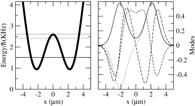
Figure 5: (left) Depiction of the potential in the $x$ direction in units of $\hbar$. The horizontal lines correspond to the single particle eigenenergies of the single particle Hamiltonian. (right) The first four single particle modes corresponding to the energies depicted in the left.

Before analyzing the binary mixtures in the next section, we will present here numerical results for the single component to illustrate the main differences between the various two-mode models and 1D reductions.

As discussed in the introduction, we consider the same setup and the same trap parameters as in the experiments of the Heidelberg group [4]. There, a condensate of ⁸⁷Rb with $1150$ atoms is confined to a fairly small region of $\sim 5\,\mu$m through the potential,

$$V({\bf r}) = {1\over 2}M(\omega_{x}^{2}x^{2}+\omega_{y}^{2}y^{2}+\omega_{z}^{2}z^{2})+V_{0}\cos^{2}(\pi x/q_{0})$$ (52)

with $\omega_{x}=2\pi\times 78$ Hz, $\omega_{y}=2\pi\times 66$ Hz, $\omega_{z}=2\pi\times 90$ Hz, $q_{0}=5.2\mu$m, and $V_{0}=413\,h$ Hz. In Fig. 5 we show the potential in the $x$ direction together with the first four energy levels of the single particle Hamiltonian and the corresponding modes. The energy levels of the single particle Hamiltonian show a clear separation between the two first eigenvalues, ground and first excited state, which are almost degenerate, and the next two.

The atom-atom interaction strength is in this case, $g=4\pi\hbar^{2}a/M$. The scattering length for ⁸⁷Rb is $a=100.87a_{B}$, therefore $g/\hbar$=0.04878 KHz $\mu m^{3}$. Noting that the number of atoms is known up to 10% in the experiment, the relevant product, $gN/\hbar$ is in the range $[51.22,60.98]$ KHz $\mu m^{3}$. Ref. [9] uses a value of 58.8 KHz $\mu m^{3}$ to simulate the experimental setup. This large value of $gN$ corresponds to a situation similar to panel (c) of Fig. 4, where the possible dynamical situations we can have are: Josephson oscillations, i.e. closed orbits around the stationary point $(z^{0},\delta\phi^{0})=(0,0)$, and self trapping regimes, usually funning phase modes.

In the experiments, the system is prepared in a slightly uneven double-well potential which produces an initial population imbalance between both sides of the barrier. At $t=0$ the asymmetry is removed and the BEC is left to evolve in a symmetric double-well potential. In our numerical simulations the initial states with either $\delta\phi(0)=0$ or $\pi$ are constructed in a different way than in the experiment. We build initial states which are by construction two-mode-like. First, we obtain numerically the ground and first excited states of the condensate in the double-well potential by solving the time independent GP equation (both for the 1D reductions and the 3D case), then use those to build the left and right modes, Eq. (4), and finally construct initial states of any given initial imbalance, $z_{0}$: $\Psi_{z_{0}}({\bf r};t=0)=\alpha\phi_{L}({\bf r})+e^{l\imath\pi}\beta\phi_{R}({\bf r})$, with $\alpha^{2}+\beta^{2}=1$ and $\alpha^{2}-\beta^{2}=z_{0}$. The ground and first excited states are obtained by a standard imaginary time evolution of the equation from an initial state with the proper parity. The density profiles of the ground, first excited and left and right modes computed numerically are plotted in Fig. 1. As can be seen, the left/right modes are indeed well localized at each side of the barrier.

From these ground and first excited states we compute all the parameters entering in the S2M and I2M descriptions presented in Secs. 3.1, and 3.2. The actual values of the parameters are, $K/\hbar=0.00799$ KHz, and $NU/\hbar=1.19841$ KHz for the S2M and $A/\hbar=1.19372$ KHz, $B/\hbar=0.03683$ KHz, and $C/\hbar=0.0023590$ KHz for the I2M . The values of the overlaps are: $N\gamma_{++}/\hbar=0.581746$ KHz, $N\gamma_{+-}/\hbar=0.59803$ KHz and $N\gamma_{--}/\hbar=0.623769$ KHz. These numbers are used to generate the comparisons to S2M or I2M in the following figures.

In the full GP3D simulations we define the number of atoms in the left well as: $N_{L}(t)=\int_{-\infty}^{0}dx\int_{-\infty}^{\infty}dy\int_{-\infty}^{\infty}dz\,\,|\Psi({\bf r};t)|^{2}\,.$ The number of atoms in the right well is computed as $N_{R}(t)=N-N_{L}(t)$. From these values, the population imbalance reads, $z(t)=(N_{L}(t)-N_{R}(t))/N$. Analogous definitions are used in the GP1D and NPSE equations.

The phase difference between both sides of the potential barrier is computed in the following way. The phase at each point at a certain time, $\phi(x,y,z;t)$, is:

$$\Psi(x,y,z;t)=\sqrt{\rho(x,y,z;t)}\exp(\imath\;\phi(x,y,z;t))\,,$$ (53)

where the local density, $\rho(x,y,z;t)=|\Psi(x,y,z;t)|^{2}\,$.

Averaged densities are defined as, i.e. integrating over the $z$ component,

$$\rho(x,y;t)=\int_{-\infty}^{\infty}dz\,\,\rho(x,y,z;t)\,.$$ (54)

To visualize the phase coherence along some of the planes we define, e.g. integrating the $z$ component,

$$\phi(x,y;t)={1\over\rho(x,y;t)}\int_{-\infty}^{\infty}dz\,\,\rho(x,y,z;t)\;\phi(x,y,z;t)\,.$$ (55)

The phase on the left, $\phi_{L}(t)$, is defined as,

$$\phi_{L}(t)={1\over N_{L}(t)}\int_{-\infty}^{0}dx\int_{-\infty}^{\infty}dy\int_{-\infty}^{\infty}dz\,\,\rho(x,y,z;t)\;\phi(x,y,z;t)\,.$$ (56)

The phase on the right is defined accordingly.

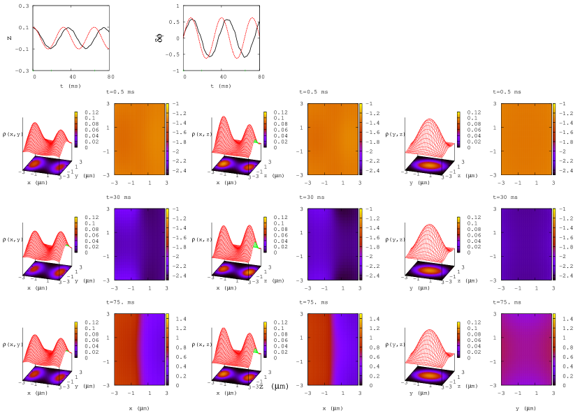
Figure 6: The two smaller plots above depict in solid-black line the GP3D time evolution of $z$ (left) and $\delta\phi$ (right), computed as explained in the text compared to the I2M predictions in dashed-red. Then we show 3D pictures complemented with contour plots, left, of $\rho(x,y;t)$, $\rho(x,z;t)$ and $\rho(y,z;t)$ at three different times, 0.5 ms (upper), 30 ms (middle) and 75 ms (lower), respectively. On the right of each plot we present a contour plot of the averaged quantum phase $\phi(x,y;t)$, $\phi(x,z;t)$ and $\phi(y,z;t)$ at the same times. They correspond to the first run presented in Fig. 8, $z(0)=0.1$ and $\delta\phi(0)=0$.

The way to implement the above averages over the phase has been done in the following way,

$$\phi(x,y;t) = {\rm arctan}{\int_{-\infty}^{\infty}dz\;{\rm Im}[\Psi(x,y,z;t)]\;\rho(x,y,z;t)\over\int_{-\infty}^{\infty}dz\;{\rm Re}[\Psi(x,y,z;t)]\;\rho(x,y,z;t)}\,,$$

$$\phi_{L}(t) = {\rm arctan}{\int_{-\infty}^{0}dx\int_{-\infty}^{\infty}dy\int_{-\infty}^{\infty}dz\;{\rm Im}[\Psi(x,y,z;t)]\;\rho(x,y,z;t)\over\int_{-\infty}^{0}dx\int_{-\infty}^{\infty}dy\int_{-\infty}^{\infty}dz\;{\rm Re}[\Psi(x,y,z;t)]\;\rho(x,y,z;t)}\;.$$

5.1 GP3D results

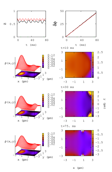
Figure 7: Similar to Fig. 6 but for a self-trapped case, $z(0)=0.7$, $\delta\phi(0)=0$, for three different times, $10,30$ and $75$ ms and showing the averages over $z$. We plot $\rho(x,y;t)$ and contour plots. On the right panels we present contour plots of the averaged quantum phase, $\phi(x,y;t)$. The phase coherence of the condensates at each side of the barrier is clearly seen.

In Figs. 6 and 7 we present full GP3D simulations for a Josephson regime and a running phase mode self-trapped case, respectively. These two figures clearly show two relevant aspects of the problem. First, it is clear that during the full time evolution, which covers up to $t=80$ ms in the figure, the system remains mostly localized on the two minima of the potential. Therefore, the density has a two-peaked structure over the considered time period. Secondly, the atoms in each of the two wells remain to a large extent in a coherent phase during all times. This can be seen from the uniform color, constant phase, at each side of the barrier in the right panels of the figures. These two characteristics of the time evolution of the 3D Gross-Pitaevskii equation support the use of two-mode approximations.

The modulation of the density profiles on the transverse direction is seen to be small, with a mostly constant quantum phase in the region populated by the atoms. This indicates that the transverse dynamics can be integrated out to a large extent, as is done in the 1D reductions discussed in Sec. 4.

The Josephson dynamics, Fig. 6, is clearly seen in the small upper panels depicting $z(t)$ and $\delta\phi(t)$. They both oscillate with the same period but with a phase-shift of $\pi/2$.

A self-trapped case is shown in Fig. 7. The atoms remain trapped mostly on the left side of the trap (they start with an imbalance of $z(0)=0.7$) and remain trapped in this potential-well during the considered time evolution. The coherence of the phase at each side of the potential barrier can also be appreciated in the figure, although here we should note that the right side of the barrier, being less populated, is concentrated on a smaller $(x,y)$ domain.

5.2 Comparison between the different models

The GP3D cases described above indicate that within the configuration considered here the two commonly employed two-mode models and 1D equations are expected to be reasonable. In this section we present comparisons between the different approaches described in the previous sections: 1D reductions (NPSE , GP1D ) and two-mode models, S2M and I2M .

5.2.1 GP3D vs 1D reductions: GP1D and NPSE 

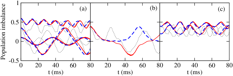
Figure 8: Dynamical evolution of the population imbalance, $z$, between both sides of the barrier for a single component condensate. Solid (red) line corresponds to the GP3D , the dashed (blue) line to the NPSE , and the dotted (black) stands for the GP1D . Panel (a) contains $\delta\phi(0)=0$ cases, with $z(0)=0.1,0.35$, and $0.6$. (b) Corresponds to the critical value, $z(0)=0.39$ and $\delta\phi(0)=0$. (c) Depicts two self-trapped cases with an initial $\delta\phi(0)=\pi$, with $z(0)=0.2$, and $0.4$.

In Fig. 8 we present the time evolution of the population imbalance for the different dynamical conditions described in Sec. 3.3, i.e. Josephson, and self-trapping. We compare the full GP3D (solid red) with the two previously described 1D reductions, GP1D (dotted black) and NPSE (dashed blue).

First, we note that the dynamics emerging from the GP3D is indeed similar to what was predicted by analyzing the S2M equations in Sec. 3.3. Qualitatively, the GP3D simulations do follow the patterns predicted by the two-mode approximations. Lets us briefly describe each of the results:

• The first panel, (a), contains simulations performed with zero initial phase difference, i.e. Josephson oscillations and self-trapping cases. For the Josephson cases, $z(0)=0.1,0.35$, the imbalance oscillates with a frequency which is mostly independent of the initial imbalance (for small imbalances). With $z(0)=0.1$ the oscillations are almost sinusoidal, while as we increase the initial imbalance their shape becomes more involved but remaining periodic. In the self-trapped case, $z(0)=0.6$, the atoms remain mostly on the initial side of the trap and there are short and small periodic oscillations as predicted by the two-mode models. At longer times, the imbalance is seen to decrease smoothly, implying a departure from the predicted two-mode dynamics [38].

  

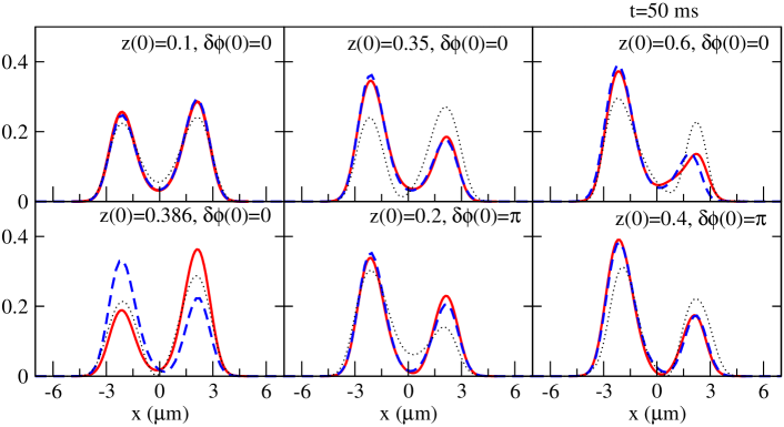
  Figure 9: Snapshots of the axial density profiles, $\rho(x;t)$ $(\mu m)^{-1}$ at $t=50$ ms calculated by means of the GP3D evolution (solid red line), the NPSE (dashed blue line), and the GP1D (dotted black line). The initial conditions correspond to the ones used to generate Fig. 8.

  The two 1D reductions give qualitatively similar results in most situations to GP3D , but not quantitatively in all cases. The NPSE is seen to reproduce very well the GP3D in all the runs up to times near $\sim 40$ ms. Above those times, the period of oscillation predicted by the NPSE is slightly shorter than the GP3D one. The GP1D on the contrary only captures the amplitude of oscillation in the Josephson cases, failing in all cases to give the same period as the GP3D or the NPSE . Moreover, the GP1D departs notably from two-mode for the self-trapped case. It does predict self trapping, but more than two modes contribute to the time evolution.

• Panel (b) is computed near the critical value of the full GP3D , $z(0)=0.39$ for $\delta\phi(0)=0$. The GP1D and NPSE predict a critical initial imbalance close to the value predicted by the GP3D .

• Panel (c) contains two self trapped cases obtained with an initial $\delta\phi(0)=\pi$ and $z(0)=0.2$, and $0.4$. Notice that for $\delta\phi(0)=\pi$ the critical imbalance is smaller. The discussion is similar to the Josephson case, i.e. the NPSE captures most of the dynamical features of the GP3D while the GP1D only provides a qualitative understanding of the problem.

These results justify the use of the NPSE in Ref. [4] to analyze their experiment.

To further explore the quality of the 1D reductions, we present in Fig. 9 the density profiles in the $x$ direction after integrating the $y$ and $z$ components, $\rho(x;t)=\int_{-\infty}^{\infty}dy\,\int_{-\infty}^{\infty}\,dz\,|\Psi(x,y,z;t)|^{2}$ at $t=50$ ms. The agreement between the NPSE and the GP3D is very good in most situations, except for the critical case, as expected. In all cases the density profiles show a clear bi-modal structure. The GP1D , as could be inferred from the previous results, does not predict the correct density profiles and, as seen in the self-trapped case, $(z(0)=0.6,\delta\phi(0)=0)$, do show the contribution of higher modes. The critical initial imbalance starting with no phase difference that we find numerically by means of the GP3D is the same as found in Ref. [9], $z_{c}=0.39$, and differs from the one reported in Ref. [4], $z_{c}=0.5$.

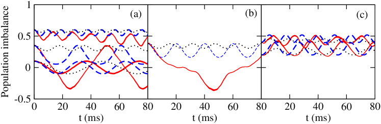
Figure 10: Dynamical evolution of the population imbalance between the two sides of the barrier for a single component condensate. The GP3D (solid red) is compared to the I2M (dashed blue) and the S2M (dotted black) results. The parameters entering in the two-mode descriptions are given in the text. Panel (a) contains runs for $\delta\phi(0)=0$, with $z(0)=0.1,0.35$, and $0.6$. (b) Corresponds to the critical value for $z(0)=0.39$ and $\delta\phi(0)=0$. (c) Depicts two self-trapped states obtained by an initial $\delta\phi(0)=\pi$, with $z(0)=0.2$, and $0.4$.

5.2.2 GP3D vs two-mode approximations, S2M and I2M 

As explained above, the use of two-mode models is suggested by the GP3D results, see Figs. 6 and 7. What is, a priori, not clear, is whether the extra assumption used in deriving the S2M (which are the most commonly employed equations) will work for each specific double-well potential. As discussed in Sec. 3.2, the conditions of the Heidelberg experiment are such that the S2M predictions are not good. This does not mean that the dynamics is not two-mode but that the overlaps involving high powers of the two localized modes are not negligible as assumed in deriving the S2M equations.

In Fig. 10 we compare GP3D (solid red), the S2M (dotted black) and the I2M (dashed blue) results using the parameters calculated microscopically from the ground and first excited state of the GP3D . Both two-mode schemes predict the same phenomenology and thus qualitatively capture the dynamics of the system. At the quantitative level, however, the I2M is clearly better. In the run with $z(0)=0.1$ and $\delta\phi(0)=0.$ (panel (a)), both the S2M and I2M predict a similar behavior with the correct amplitude and oscillation period close to the GP3D one. As the imbalance is increased, e.g. ([4] considers $z(0)=0.28$), the S2M fails to describe the correct period and predicts smaller amplitudes. This is analyzed in full detail in Ref. [9]. The critical initial imbalances determined by both two-mode approaches are smaller than the GP3D one. For the latter they predict a self-trapped case, see panel (b). Finally, for the self-trapped cases with $\delta\phi(0)=\pi$ (panel (c)) the I2M give similar oscillation amplitudes with shorter periods than the GP3D . The S2M fails both in reproducing the amplitudes and the periods.

6 Numerical solutions of the 3D Gross-Pitaevskii equations: binary mixture

As discussed in Sec. 2, one feasible way of experimentally prepare binary mixtures of BECs is to consider a number of atoms populating the $m=\pm 1$ Zeeman components of an ⁸⁷Rb $F=1$ spinor. The experimental observation of Josephson tunneling phenomena by the Heidelberg group seems to be possibly extended to trap both Zeeman components [34]. In this case the two components of the mixture have the same mass, $M\equiv m_{a}=m_{b}$, and equal intra-species interactions, $g_{aa}=g_{bb}\equiv g$. With respect to the inter-species interaction we will consider the case of ⁸⁷Rb which implies $g_{ab}\sim g$.

The mean field GP3D system of equations governing the dynamics of the three components of an $F=1$ spinor BEC can be written as [39],

$$i\hbar{\partial\psi_{\pm 1}\over\partial t} = [{\cal H}_{s}+c_{2}(n_{\pm 1}+n_{0}-n_{\mp 1})]\psi_{\pm 1}+c_{2}\psi_{0}^{2}\psi^{*}_{\mp 1}\,,$$

$$i\hbar{\partial\psi_{0}\over\partial t} = [{\cal H}_{s}+c_{2}(n_{1}+n_{-1})]\psi_{0}+c_{2}2\psi_{1}\psi_{0}^{*}\psi_{-1}\,,$$ (58)

with ${\cal H}_{s}=-\hbar^{2}/(2M)\,{\bm{\nabla}}^{2}+V+c_{0}n$ being the spin-independent part of the Hamiltonian. The density of the $m$-th component is given by $n_{m}({\bf r})=|\psi_{m}({\bf r})|^{2}$, while $n({\bf r})=\sum_{m}|\psi_{m}({\bf r})|^{2}$ is the total density normalized to the total number of atoms $N$. The couplings are $c_{0}=4\pi\hbar^{2}(a_{0}+2a_{2})/(3M)$ and $c_{2}=4\pi\hbar^{2}(a_{2}-a_{0})/(3M)$, where $a_{0}$ and $a_{2}$ are the scattering lengths describing binary elastic collisions in the channels of total spin 0 and 2, respectively. Their values for ⁸⁷Rb are $a_{0}=101.8a_{B}$ and $a_{2}=100.4a_{B}$ [40]. Since the spin-dependent coupling, $c_{2}$, is much smaller than the spin-independent one, $c_{0}$, and the total number of atoms that we will consider is relatively small $N=1150$, the population transfer between the different components can be neglected [30]. Therefore, in our calculation the number of atoms in each sublevel remains constant in time allowing to treat the system as a real binary mixture of components $a$ and $b$. Comparing the system of Eqs. (LABEL:GP-mixture) and (58) the value of the couplings can be read off, $g_{aa}=g_{bb}=c_{0}+c_{2}$ and $g_{ab}=g_{ba}=c_{0}-c_{2}$.

Once the total number of atoms is fixed we want to investigate the Josephson-like dynamics for different number of atoms populating each component $N_{a}=f_{a}N$ and $N_{b}=f_{b}N$ and for different initial conditions $z_{a}(0)$, $z_{b}(0)$, $\delta\phi_{a}(0)$ and $\delta\phi_{b}(0)$.

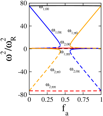
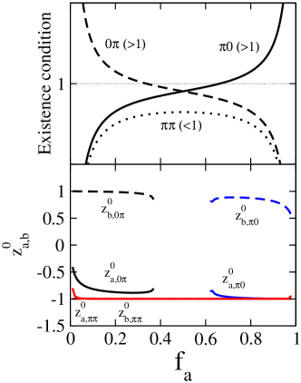
Figure 11: (left) Values of the frequencies, $\omega/\omega_{R}$, listed in Table 3 for the specific conditions considered in the numerical simulations as a function of the fraction of atoms in the $a$ component, $f_{a}$. The notation is as follows, $\omega_{i;\alpha\beta}$, with $i=1,2$ and $\alpha,\beta=0,\pi$. (right) The conditions for the existence of the non-trivial equilibrium points given in Eqs. (38, 41, 45), upper panel, as function of $f_{a}$ for the conditions described in the text. The lower panel contains the explicit equilibrium points $z_{a}^{0},z_{b}^{0}$ as a function of $f_{a}$ obtained by solving equations (34). Note that each equilibrium point has a trivial partner which is obtained by flipping the sign of $z_{a}^{0},z_{b}^{0}$.

The values of $\Lambda=NU/\hbar\omega_{R}$ and $\tilde{\Lambda}=N\tilde{U}/\hbar\omega_{R}$ are $\Lambda=74.278$ and $\tilde{\Lambda}=74.968$. With $\Lambda/\tilde{\Lambda}=0.99$. These are obtained from the microscopic 3D parameters computed in the scalar case, with the same total number of particles, Sec. 5. This is reasonable for the case we are considering where $g_{aa}=g_{bb}\sim g_{ab}$, which implies that the ground state wave functions for the GP equations of the mixture do not depend on $f_{a}$ and $f_{b}$ for a fixed total number of particles. This would certainly not be the case if $g_{aa}=g_{bb}\neq g_{ab}$, in such case one would need to recompute the ground state wave functions for $a$ and $b$ for each value of $f_{a}$.

Following the discussion in Sec. 3.6, where the predictions of the S2M were discussed in detail, the system has the trivial equilibrium points, listed in Table 3 with $\beta=0.009$. In Fig. 11 we show the values of the two eigenfrequencies for each of the trivial equilibrium points listed in Table 3 for the specific conditions described above. The figure shows a number of important features about the stability of the trivial equilibrium points. First, the $(z_{a}^{0},\delta\phi_{a}^{0},z_{b}^{0},\delta\phi_{b}^{0})=(0,0,0,0)$ is always stable regardless of the total polarization of the system (measured by $f_{b}-f_{a}$). Second, the $(z_{a}^{0},\delta\phi_{a}^{0},z_{b}^{0},\delta\phi_{b}^{0})=(0,\pi,0,\pi)$ mode is always unstable, as seen by the negative value taken by the square of the frequencies. Third, the $(z_{a}^{0},\delta\phi_{a}^{0},z_{b}^{0},\delta\phi_{b}^{0})=(0,0,0,\pi)$ mode should be stable for $f_{a}\lesssim 0.43$, correspondingly the $(z_{a}^{0},\delta\phi_{a}^{0},z_{b}^{0},\delta\phi_{b}^{0})=(0,\pi,0,0)$ is stable for $f_{b}\lesssim 0.43$ and therefore there is a range of polarizations, given by $0.43\gtrsim f_{a}\lesssim 0.57$ where the only trivial mode which is stable is the $(z_{a}^{0},\delta\phi_{a}^{0},z_{b}^{0},\delta\phi_{b}^{0})=(0,0,0,0)$.

The non-trivial equilibrium points in this case can be obtained by analyzing the conditions given in Sec. 3.6. For $(\delta\phi_{a}^{0},\delta\phi_{b}^{0})=(0,0)$ there are no equilibrium points apart from the trivial one, due to $\Lambda\sim\tilde{\Lambda}$. In the other three cases there are non-trivial equilibrium points depending on the specific values of $f_{a}$. In Fig. 11(right) we analyze their existence. First, we note that there are non-trivial points corresponding to $(\delta\phi_{a}^{0},\delta\phi_{b}^{0})=(0,\pi)$ provided $f_{a}\lesssim 0.37$, correspondingly there are also equilibrium points for $(\delta\phi_{a}^{0},\delta\phi_{b}^{0})=(0,\pi)$ if $f_{b}\lesssim 0.37$. There is also a non-trivial equilibrium point for $(\delta\phi_{a}^{0},\delta\phi_{b}^{0})=(\pi,\pi)$ regardless of $f_{a}$. As can be seen in the figure, all these non-trivial equilibrium points correspond to fairly imbalanced conditions and can in most cases be understood in simple terms from the analysis of the scalar case. For instance, the equilibrium point for $(\delta\phi_{a}^{0},\delta\phi_{b}^{0})=(\pi,\pi)$ corresponds to $z_{a}^{0}\sim z_{b}^{0}\sim 1$ (or $-$1), which can be understood as having both components locked in a $\pi$-mode. Similarly, the equilibrium points in the $(0,\pi)$ or $(\pi,0)$ cases exist whenever the most abundant component is populated enough to drive the dynamics close to being $\pi$ locked.

6.1 GP3D calculations: phase coherence and localization

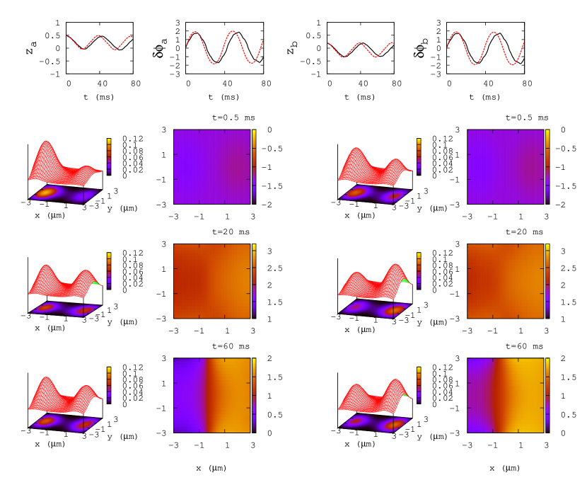
Figure 12: Full GP3D calculations of the dynamics of a binary mixture with $z_{a}(0)=0.5$, $z_{b}(0)=0.2$, $\delta\phi_{a}(0)=0$, $\delta\phi_{b}(0)=0$, $f_{a}=0.25$ and $f_{b}=0.75$. The upper four plots depict, from left to right, $z_{a}(t)$, $\delta\phi_{a}(t)$, $z_{b}(t)$, and $\delta\phi_{b}(t)$ in solid black compared to the I2M prediction, dashed-red . Then each row contains from left to right: 3D depictions complemented by contour plots of $\rho_{a}(x,y;t)$, a contour plot of the averaged phase $\phi_{a}(x,y;t)$, 3D depictions complemented by contour plots of $\rho_{b}(x,y;t)$, and a contour plot of the averaged phase $\phi_{b}(x,y;t)$. Each row corresponds to a different time, .5 ms (upper), 20 ms (middle) and 60 ms (lower), respectively.

The numerical solutions of the GP3D presented in Sec. 5 for the single component case showed two features. First, the atoms remained mostly localized in the two minima of the potential well and secondly, each group of atoms had to a large extent the same quantum phase. This, clearly supported the picture of having two BEC, one at each side of the barrier, with a well defined phase at each side during the dynamical evolution. Essentially those are the premises used to derive the two-mode models, both for single component and for binary mixtures, as we did in Sec. 3.

As in the scalar case, our exact GP3D numerical solutions of the dynamics of the binary mixture in several initial conditions of population imbalances and phase differences show two distinctive features, see Fig. 12. First, the density of atoms for each component is always bi-modal, with the two atom bunches centered around the minima of the potential well. Secondly, the phase of the wave function is mostly constant for each species at each side of the potential trap. Thus, we find that the GP3D does predict the dynamics to be mostly bi-modal also for the binary mixture case.

At the end of the section we will consider some deviations from the bi-modal behavior that are found in very specific conditions, e.g. for very large population imbalances and also when analyzing a case with $g_{ab}\neq g_{aa}=g_{bb}$.

6.2 Small oscillations around $z_{a,b}^{0}$ and $\delta\phi_{a,b}^{0}=0$

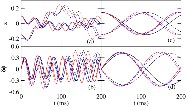
Figure 13: Behavior of the population imbalance, $z_{a}(t)$ (solid lines), and $z_{b}(t)$ dashed lines, and phase difference, $\delta\phi_{a}(t)$ (solid lines) and $\delta\phi_{b}(t)$ (dashed lines), computed using GP3D (black lines), NPSE (blue lines), and I2M (red lines) in a polarized case, $f_{a}=0.8$, left, and a zero polarization case, $f_{a}=0.5$, right, respectively. The initial conditions are $z_{a}(0)=0.1$, $z_{b}(0)=-0.15$ and $\delta\phi_{a}(0)=\delta\phi_{b}(0)=0$ for the left panels, and $z_{a}(0)=-z_{b}(0)=0.15$ and $\delta\phi_{a}(0)=\delta\phi_{b}(0)=0$ for the right panels.

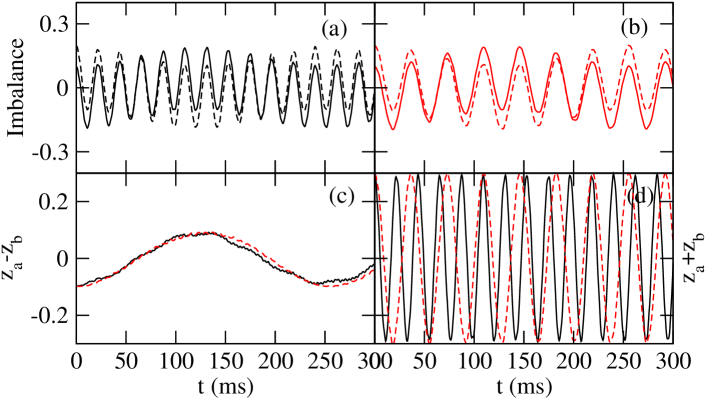
Figure 14: Behavior of the population imbalance in NPSE (red) and GP1D (black) simulations in the zero magnetization case, $f_{a}=f_{b}$. The initial conditions are $z_{a}(0)=0.1$, $z_{b}(0)=0.2$ and $\delta\phi(0)=0$. The upper panels correspond to (a) $z_{a}(t)$ (solid line) and $z_{b}(t)$ (dashed line) obtained with the GP1D equations, (b) $z_{a}(t)$ and $z_{b}(t)$ obtained with the NPSE equations, (c) behavior of $z_{a}(t)-z_{b}(t)$ for GP1D (solid) and NPSE (dashed), and (d) behavior of $z_{a}(t)+z_{b}(t)$.

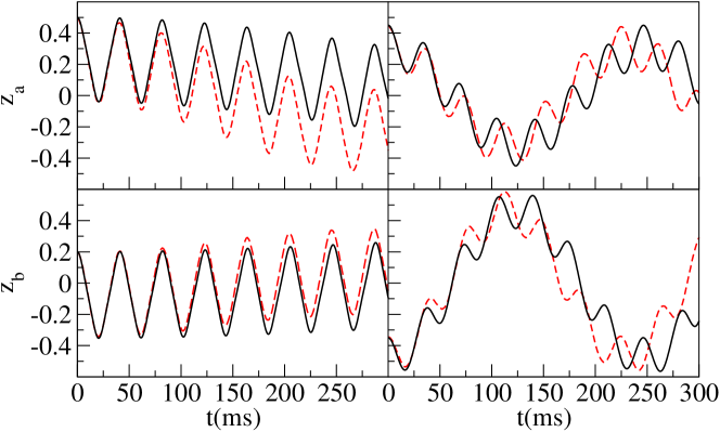
Figure 15: (left panels) Evolution of the population imbalance of each component for a binary mixture with $f_{a}=0.25$. The upper panel shows $z_{a}(t)$, and the bottom panel $z_{b}(t)$. The solid (black) line corresponds to the I2M model and the dashed (red) line to the NPSE . The initial conditions are $z_{a}(0)=0.5$, $z_{b}(0)=0.2$, $\delta\phi_{a}(0)=\delta\phi_{b}(0)=0$. (right panels) As in the left panel, but with $f_{a}=0.6$ and initial conditions $z_{a}(0)=0.45$, $z_{b}(0)=-0.35$, $\delta\phi_{a}(0)=\delta\phi_{b}(0)=0$.

The two predictions of the S2M described in Sec. 3.6 are confirmed by the NPSE and GP1D simulations as can be seen in Figs. 13 and 14. In Fig. 13 (left panels) we consider a very polarized case, $f_{a}=0.8$. As expected from the two-mode analysis the dynamics of the most populated component should to a large extent decouple from the less populated one and perform fast Josephson oscillations with a frequency close to the corresponding one for the scalar case, $\omega_{J}=\omega_{R}\sqrt{1+\Lambda}$. The GP3D simulation is seen to confirm the above and follow closely the predictions of the I2M . The less abundant component is strongly driven by the most populated one and shows an anti-Josephson behavior as described in Ref. [30].

Another prediction is related to the behavior of $z_{a}+z_{b}$ and $z_{a}-z_{b}$ in the non-polarized case, $f_{a}=f_{b}$. As explained in Sec. 3.6, in this case the difference, $z_{a}-z_{b}$, should enhance the long mode which oscillates with the Rabi frequency of the system, while the sum $z_{a}+z_{b}$ should mostly oscillate with the Josephson frequency. In the right part of Fig. 13 we present the extreme case when $z_{a}(0)=-z_{b}(0)$ computed with GP3D , NPSE and I2M . In this case, both population imbalances and phase differences oscillate mostly with the Rabi frequency of the system, keeping during the time evolution $z_{a}+z_{b}\sim 0$.

As seen in Fig. 14 both 1D reductions produce qualitatively similar physics. The only important difference is that the frequency of the Josephson oscillations is higher in the GP1D , as occurred already for the single component, see Sec. 5.

Interestingly, they predict different Josephson oscillations while the Rabi frequencies are similar. In panel (c) of Fig 14 the long oscillation corresponding to the Rabi mode is seen to agree well with the corresponding long oscillation seen in the right panels of Fig. 13. The Josephson-like oscillations of binary mixtures of spinor $F=1$ ⁸⁷Rb BECs around the $(z_{a}^{0},\delta\phi_{a}^{0},z_{b}^{0},\delta\phi_{b}^{0})=(0,0,0,0)$ are therefore essentially controlled by two frequencies, $\omega_{R}$ and $\omega_{J}$.

As a general statement, in the conditions of the Heidelberg experiment, as occurred for the scalar case, the I2M produces more reliable results than the S2M model, which are not shown in the figures. Notice that the parameters that we use for the I2M are extracted from the GP3D calculation as given in Sec. 5. Other representative cases with $(\delta\phi_{a}(0),\delta\phi_{b}(0))=(0,0)$ but with larger initial imbalances, $z_{i}(0)\sim 0.5$ are shown in Fig. 15. On the left side of the figure we show the population imbalance of each component for a simulation with $f_{a}=0.25$. In this case the dynamics is controlled by $\omega_{J}$. The panel on the right depicts a simulation with $f_{a}=0.6$ and close to opposite initial population imbalances. In this case, both frequencies $\omega_{J}$ and $\omega_{R}$ show up in the evolution. The I2M provides a satisfactory description of the dynamics.

6.3 Small oscillations around $z^{0}_{a,b}$, $\delta\phi^{0}_{a}=0$ and $\delta\phi^{0}_{b}=\pi$

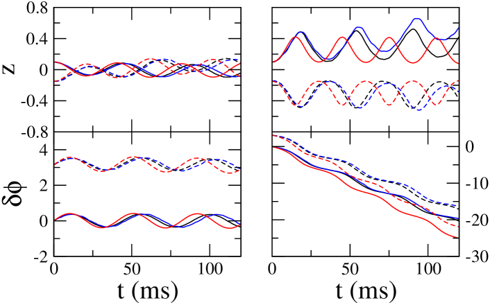
Figure 16: Two simulations with the same initial conditions, $z_{a}(0)=0.1$, $z_{b}(0)=-0.15$, $\delta\phi_{a}(0)=0$ and $\delta\phi_{b}(0)=\pi$ but with different compositions of the mixture. The case on the left has $f_{a}=0.2$ while the case on the right $f_{a}=0.8$. The blue lines are obtained by means of a full GP3D , the black lines are the NPSE results, and the red lines are the I2M results. Solid and dashed lines correspond to the $a$ and $b$ components, respectively.

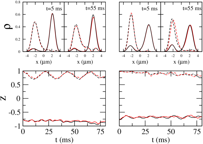
Figure 17: Two simulations with the same initial conditions, $z_{a}(0)=-0.78$, $z_{b}(0)=0.99$, $\delta\phi_{a}=0$ and $\delta\phi_{b}=\pi$, but with different composition. The case on the left has $f_{a}=0.1$ while the case on the right $f_{a}=0.9$. The red lines are obtained by means of a full GP3D while the black lines are the NPSE results. Solid and dashed lines correspond to the $a$ and $b$ components, respectively.

As explained above, for these conditions there can exist up to three stationary points depending on the specific value of $f_{a}$ considered. The trivial equilibrium point exists provided $f_{a}\lesssim 0.43$, see Fig. 11. This prediction of the two-mode models is observed both in the GP3D and NPSE as it can be seen in Fig. 16. In the figure, we consider a simulation with $z_{a}(0)=0.1$, $z_{b}(0)=-0.15$, and $f_{a}=0.2<0.43$ (left panels). The population imbalance (upper panel) of both components oscillates in the usual Josephson regime. At the same time, the phase difference oscillates with its characteristic phase-shisft of $\pi/2$ with respect to the imbalance (lower panel). The phase of the $a$ component oscillates around $\delta\phi_{a}=0$ while $\delta\phi_{b}$ does oscillate around $\delta\phi_{b}=\pi$.

A completely different picture emerges when the fraction of atoms in both components is exchanged, $f_{a}=0.8>0.43$ (right panels), with most of the atoms populating the $a$ component. In this case, the oscillation amplitude is large, both components remain trapped on their original sides and the phase difference becomes unbounded. This should be considered as a genuine effect of the binary mixture as each component follows a running phase mode at each side of the potential barrier.

The comparison between the NPSE and GP3D is very satisfactory. The NPSE captures almost completely the dynamics up to times of 100 ms. In all cases, the NPSE reproduces correctly both the phase difference and population imbalance. The only sizeable discrepancies occur for times $\gtrsim 80$ ms in the run without equilibrium point (right panel).

The I2M gives a good qualitative picture of both cases but fails to provide predictions as accurate as the NPSE , as happened in the scalar case, see for instance Figs. 8 and  10. In particular the predicted periods of oscillation are much longer than the actual ones.

An example of simulations around non-trivial equilibrium points is presented in Fig. 17. As explained previously, these involve very large and opposite initial population imbalances for both components. In Fig. 17 we consider a case with initial conditions very close to the predicted equilibrium point using the standard two-mode, and described in Fig.11, $z_{a}(0)=-0.78$, and $z_{b}(0)=0.99$, with $f_{a}=0.1$. Also in the same figure we consider a similar run but with $f_{a}=0.9$. In both cases the NPSE and GP3D predict a very similar dynamics. These simulations will be discussed again in Sec. 6.5 as they exhibit effects which clearly go beyond a two-mode approximation.

6.4 Small oscillations around $z^{0}_{a,b}$ and $\delta\phi^{0}_{a,b}=\pi$

The trivial equilibrium point is not stable in the considered conditions as seen in Fig. 11. The non-trivial one, however, is only attainable if extremely imbalanced configurations for both components are considered. This case would correspond essentially to having both components in a $\pi$ mode state, which in our conditions only exists for $z~{}\sim 1$ as can be seen in the blue spots in panel (c) of Fig. 4. In Fig. 18 we present two simulations with different initial conditions. First, we consider a simulation with $z_{a}(0)=0.4$ and $z_{b}(0)=-0.2$, with $f_{a}=0.9$. The behavior is understood in simple terms, the most populated component remains self-trapped while the other component is forced by the other one. The phase evolves unbounded. The figure again contains GP3D and NPSE simulations.

The second simulation (right panels) is closer to a non-trivial equilibrium point, we consider $z_{a}(0)=0.9$ and $z_{b}(0)=0.85$ with $f_{a}=0.9$. In this case, both components remain self trapped, the phase difference is unbounded, but we do not get the expected behavior of two $\pi$ modes because the initial imbalances are not close enough to $z^{0}\sim 1$.

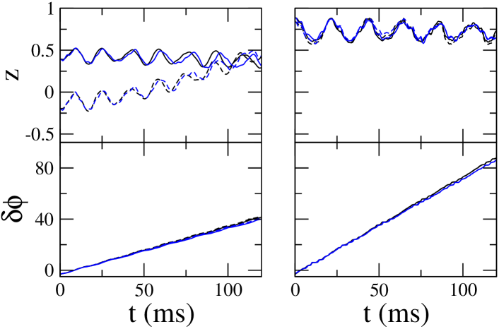
Figure 18: Two simulations corresponding to (left) $z_{a}(0)=0.4$, $z_{b}(0)=-0.2$, $\delta\phi_{a}(0)=\pi$, $\delta\phi_{b}(0)=\pi$ and $f_{a}=0.9$, and (right) $z_{a}(0)=0.9$, $z_{b}(0)=0.85$, $\delta\phi_{a}(0)=\pi$, $\delta\phi_{b}(0)=\pi$ and $f_{a}=0.9$ The blue lines are obtained by means of a full GP3D while the black lines are the NPSE results. Solid and dashed lines correspond to the $a$ and $b$ components, respectively.

6.5 Effects beyond two-mode

Most of the dynamics described in the previous sections can to a large extent be understood within the two-mode models developed in Sec. 3. There are, however, a number of situations where the two-mode fails. Some are a direct consequence of having two components evolving in the same double-well potential, others are due to having initial configurations, mostly with large initial imbalances, producing situations where the atom-atom interaction energy per atom is comparable to the gap between the first excited state and the second/third excited states.

We can distinguish two different cases: (a) involving excitations along the coordinate which contains the barrier, (b) involving excitations of the transversal coordinates.

An example of (a) is seen in Fig. 17. There, as clearly seen in the density profiles along the $x$ direction, the two-mode approximation is clearly not valid. The simplest way of seeing this is by noting the zero in the density of one of the components at $x\sim 2\mu$ m. This effect beyond two-mode is well taken care of by the NPSE which reproduces the density profile quite well during most of the time evolution considered in the simulation. Thus, the excitations of higher modes along the direction which has not been integrated out in the 1D reduction do not pose a great difficulty to the 1D reductions.

The second type, (b), of effects beyond two-mode involve excitations of the transverse components. These effects are present in any binary mixture calculation whenever the intra- and inter-species interactions are not equal. To enhance this effect, and also to explore the interesting symmetry breaking phenomena described in Ref. [25], we consider a case with $g_{aa}=g_{bb}$, but with $g_{ab}=g_{ba}=2.3g_{aa}$. Therefore, now the inter-species interaction strength is larger than the intra-species one. The two-mode prediction for this case, S2M , which was analyzed in Ref. [25] shows a large symmetry breaking pattern during the time evolution of the system. In Fig. 19 we consider a full GP3D simulation of a representative example with $z_{a}(0)=-0.2$, $z_{b}(0)=0.1$, $\delta\phi_{a}(0)=\delta\phi_{b}(0)=0$, and $f_{a}=0.7$.

The qualitative prediction of the I2M also shows the symmetry breaking, and the two components do separate from each other and mostly concentrate on one of the wells as time evolves. But, as it can be seen in the 3D depictions of $\rho(x,y;t)$ at three different times, the evolution of the system departs almost from the beginning from the two-mode. At $t=1$ ms we have the density distributions of each component corresponding to a small initial imbalance. Then at $t=11$ ms, we can already see that the most populated component is expelling the other one from the minima of the potential. This fact can be appreciated as a four peaked distribution, $\rho_{b}(x,y;t)$. After that, each of the components start to accumulate on their original sides following qualitatively the prediction of the I2M and thus presenting the symmetry breaking pattern discussed in Ref. [25]. The two-mode approximation is in this case broken for a short period of time, when the first modes along the transverse directions are excited due to the large inter-species interaction.

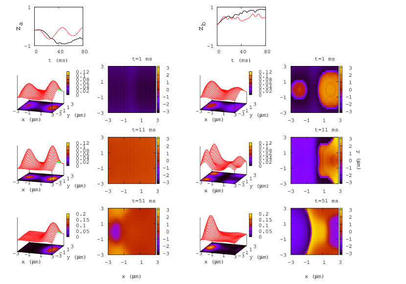
Figure 19: Full GP3D calculations of the dynamics of a binary mixture with $z_{a}(0)=-0.2$, $z_{b}(0)=0.1$, $\delta\phi_{a}(0)=0$, $\delta\phi_{b}(0)=0$, $f_{a}=0.7$ and $f_{b}=0.3$. As explained in the text in this case, $g_{aa}=g_{bb}$ and $g_{ab}=2.3g_{aa}$. The upper two plots depict $z_{a}(t)$ (left) and $z_{b}(t)$ (right). Then each row contains from left to right: 3D depictions complemented by contour plots of $\rho_{a}(x,y;t)$, a contour plot of the averaged phase $\phi_{a}(x,y;t)$, 3D depictions complemented by contour plots of $\rho_{b}(x,y;t)$, and a contour plot of the averaged phase $\phi_{b}(x,y;t)$. Each row corresponds to a different time, 1 ms (upper), 11 ms (middle) and 51 ms (lower), respectively. In all cases, solid black lines are computed with GP3D and dashed red ones with I2M .

7 Conclusions

We have presented a thorough investigation of the mean-field dynamics of a binary mixture of Bose-Einstein condensates trapped in a double-well potential. The rich dynamical regimes which take place in binary mixtures, like double self-trapped modes, Josephson oscillations, or zero and $\pi$ bound phase modes, have been scrutinized by performing full GP3D simulations covering all the relevant initial conditions. The 3D numerical solutions of the Gross-Pitaevskii equations have been used as a benchmark to critically discuss the validity of the most common 1D reductions of the GP equations, GP1D and NPSE , and the often employed simple two-mode reductions, S2M and I2M .

The full 3D solutions of the binary mixture have shown to have a large amount of phase coherence and localization at each side of the potential barrier for both components, predicting a dynamics which is mostly bi-modal. This feature permits to speak of Bose-Einstein condensates at each side of the barrier, where the atoms mostly share a common phase, and to support the use of two-mode approximations, which analytical solutions allow to gain physical insight into the problem.

To fix the conditions of the dynamics, we have focused in one particular setup that corresponds to a natural extension of the experiments reported in Ref. [4]: the case of a binary mixture made by populating two of the Zeeman states of an $F=1$ ⁸⁷Rb condensate. As discussed in the present paper, this setup already allows to observe and characterize a large variety of phenomena which are genuine of the binary mixture, e.g. anti-Josephson oscillations in highly polarized cases, long Rabi-like oscillating modes, zero and $\pi$ locked modes, etc.

For the sake of completeness and to better frame the physics of the binary mixture we have provided a detailed description of the single component dynamics, with explicit expressions for all the commonly employed approximations to the 3D mean field Gross-Pitaveskii equation. The natural extension of the latter to the binary mixture, i.e. S2M and I2M equations and 1D reductions, have been consistently derived providing a self-contained reference, easy to read, with all the relevant formulae used in the article.

The standard two-mode model, with its microscopic parameters computed with the GP3D , has been used to reexamine the existence and stability of the different regimes that can occur in both single component and binary mixture condensates, describing the Josephson oscillations and the macroscopic quantum self-trapping, including running phase modes and zero- and $\pi-$modes.

The comparisons between the two-mode models and the numerical solutions of the GP3D show an excellent agreement for conditions close to the stable stationary regimes predicted by the two-mode models. As we depart from those stable points, the S2M fails to provide a quantitative agreement with the results obtained with the GP3D equations. The range of validity of the I2M is much larger, fully capturing the dynamics of single and binary mixtures for a larger set of initial conditions.

The two most commonly employed dimensional reductions of the GP3D , the GP1D and NPSE , have been shown to differ substantially among each other, with the NPSE being clearly in much better agreement with the original 3D dynamics in a broader set of conditions. In general, the GP1D describes essentially the correct physics but quantitatively far from the GP3D predictions. Also, for self-trapped cases already in the single component case, it departs from the two-mode behavior earlier than the GP3D or the NPSE . The agreement between the NPSE and the full 3D dynamics is astonishingly good both for single component and the considered binary mixtures, where the intra- and inter-species are very similar and the NPSE equations are particularly easy to handle. This agreement is not only seen on fully integrated magnitudes, for instance population imbalances, but also on the density profiles predicted along the direction hosting the barrier.

We have also considered two situations where the two-mode approximation fails. This is naturally due to the excitation of higher modes. Two different cases have been described, first the excitation of modes in the direction of the barrier and secondly, excitation of modes in the transverse direction. The NPSE has been shown to capture perfectly the excitations along the barrier direction, reproducing the integrated density profiles obtained with the GP3D . The second case has been studied in a simulation performed with different intra- and inter-species, which can be achieved in principle experimentally through Feshbach resonance modulation of the scattering lengths. In this case, the dynamics of the less populated component in each side of the trap departs notably from the two-mode with clear excitations of transverse modes, seen already in the density profiles along a transverse direction.

The present article is intended both to motivate the experimental effort to study binary mixtures of BECs, where we have shown that a large variety of phenomena related to phase coherence and localization can be observed, and to serve as a tool in the analysis of such experiments providing a concise and self-contained derivation of the most commonly used models.

References

- [1] A. J. Leggett, Rev. Mod. Phys. 73, 307 (2001).
- [2] L. Pitaevskii, and S. Stringari, Bose-Einstein Condensation. (Oxford University Press, Oxford, 2003).
- [3] M. R. Andrews, C. G. Townsend, H.-J. Miesner, D. S. Durfee, D. M. Kurn, and W. Ketterle, Science 275, 637 (1997).
- [4] M. Albiez, R. Gati, J. Fölling, S. Hunsmann, M. Cristiani, and M. K. Oberthaler, Phys. Rev. Lett. 95, 010402 (2005).
- [5] A. Smerzi, S. Fantoni, S. Giovanazzi, and S. R. Shenoy, Phys. Rev. Lett. 79, 4950 (1997).
- [6] S. Raghavan, A. Smerzi, S. Fantoni, and S. R. Shenoy, Phys. Rev. A 59, 620 (1999).
- [7] G.J. Milburn, J. Corney, E. M. Wright, and D. F. Walls, Phys. Rev. A 55, 4318 (1997).
- [8] A. P. Tonel, A. Foerster and J. Links, Journal of Physics A 38 1235 (2005).
- [9] D. Ananikian and T. Bergeman, Phys. Rev. A 73, 013604 (2006).
- [10] R. Gati and M. K. Oberthaler, J. Phys. B: At. Mol. Opt. Phys. 40, R61 (2007).
- [11] M. Jääskeläinen, and P. Meystre, Phys. Rev. A, 71, 043603 (2005), M. Jääskeläinen, and P. Meystre, Phys. Rev. A 73, 013602 (2006).
- [12] J. I. Cirac, M. Lewenstein, K. Molmer, P. Zoller, Phys. Rev. A 57, 1208 (1998).
- [13] J. Javanainen, M. Yu. Ivanov, Phys. Rev. A 60, 2351 (1999).
- [14] P. Ziń, J. Chwedeńczuk, B. Oleś, K. Sacha and M. Trippenbach, Euro. Phys. Lett. 83 64007 (2008).
- [15] K. Sakmann, A. I. Streltsov, O. E. Alon, and L. S. Cederbaum, Phys. Rev. Lett. 103, 220601 (2009).
- [16] B. Juliá-Díaz, D. Dagnino, M. Lewenstein, J. Martorell, A. Polls, Phys. Rev. A 81, 023615 (2010).
- [17] B. Juliá-Díaz, J. Martorell, A. Polls, in press Phys. Rev. A (2010).
- [18] L. D. Carr, D. R. Dounas-Frazer and M. A. Garcia-March, Europhysics Letters, 90, 10005 (2010).
- [19] E. Boukobza, M. Chuchem, D. Cohen, and A. Vardi, Phys. Rev. Lett. 102, 180403 (2009).
- [20] M. Albiez, PhD Thesis, U. Heidelberg (2005).
- [21] L. Salasnich, A. Parola, and L. Reatto, Phys. Rev. A 65, 043614 (2002).
- [22] S. Ashab and C. Lobo, Phys. Rev. A 66, 013609 (2002).
- [23] H. T. Ng, C. K. Law, and P.T. Leung, Phys. Rev. A 68, 013604 (2003); L. Wen and J. Li, Phys. Lett. A 369, 307 (2007).
- [24] X-Q. Xu, L-H. Lu and Y-Q. Li, Phys. Rev. A 78, 043609 (2008).
- [25] I. I. Satija, R. Balakrishnan, P. Naudus, J. Heward, M. Edwards, and C. W. Clark, Phys. Rev. A 79, 033616 (2009).
- [26] G. Mazzarella, M. Moratti, L. Salasnich. M. Salerno, and F. Toigo, J. Phys. B: At. Mol. Opt. Phys. 43, 065303 (2010).
- [27] B. Sun and M. S. Pindzola, Phys. Rev. A 80, 033616 (2009).
- [28] A. Nadeo, R. Citro, arXiv:1003.0123.
- [29] G. Mazzarella, M. Moratti, L. Salasnich, and F. Toigo, J. Phys. B: At. Mol. Opt. Phys. 43, 065303 (2010).
- [30] B. Juliá-Díaz, M. Guilleumas, M. Lewenstein, A. Polls, and A. Sanpera, Phys. Rev. A 80, 023616 (2009).
- [31] W. Wang, J. Phys. Soc. Jpn.78, 9, 094002 (2009).
- [32] H. Pu, W. P. Zhang, and P. Meystre, Phys. Rev. Lett. 89, 090401 (2002); Ö. E. Müstecaplioglu, W. Zhang, and L. You, Phys. Rev. A 75, 023605 (2007).
- [33] B. Juliá-Díaz, M. Melé-Messeguer, M. Guilleumas, and A. Polls, Phys. Rev. A 80, 043622 (2009).
- [34] M. Oberthaler, private communication.
- [35] M. Olshanii, Phys. Rev. Lett. 81, 938 941 (1998).
- [36] W. Zhang, and L. You, Phys. Rev. A 71, 025603 (2005).
- [37] L. Salasnich and B. A. Malomed, Phys. Rev. A 74, 053610 (2006).
- [38] B. Juliá-Díaz, M. Mele-Messeguer, A. Polls, in preparation.
- [39] T.-L. Ho, Phys. Rev. Lett. 81, 742 (1998); T. Ohmi and K. Machida, J. Phys. Soc. Jpn. 67, 1822 (1998); M. Moreno-Cardoner, J. Mur-Petit, M. Guilleumas, A. Polls, A. Sanpera, and M. Lewenstein, Phys. Rev. Lett. 99, 020404 (2007).
- [40] E. G. M. van Kempen, S. J. J. M. F. Kokkelmans, D. J. Heinzen, and B. J. Verhaar, Phys. Rev. Lett. 88, 093201 (2002).