A high-order public domain code for direct numerical simulations of turbulent combustion

Abstract

A high-order scheme for direct numerical simulations of turbulent combustion is discussed. Its implementation in the massively parallel and publicly available Pencil Code is validated with the focus on hydrogen combustion. Ignition delay times (0D) and laminar flame velocities (1D) are calculated and compared with results from the commercially available Chemkin code. The scheme is verified to be fifth order in space. Upon doubling the resolution, a 32-fold increase in the accuracy of the flame front is demonstrated. Finally, also turbulent and spherical flame front velocities are calculated and the implementation of the non-reflecting so-called Navier-Stokes Characteristic Boundary Condition is validated in all three directions.

1 Introduction

Modeling of turbulence is one of the largest research areas within flow mechanics. Turbulent combustion inherits all the properties of non-reacting turbulent flow. The most important addition is linked to the highly nonlinear reaction processes, and models for this are called combustion models. Two additional challenges in turbulent combustion are the very sharp changes in density and differential diffusion of mass and heat.

For combustion processes it is crucial to be able to simulate the mixing of the combustible species correctly. Traditionally this has been done by means of mixing models in Reynolds Averaged Navier Stokes (RANS) codes by combining, e.g., the $k$-$\epsilon$ turbulence model and the eddy dissipation concept (or EDC) “mixing” model [23, 20, 22], or in Large Eddy Simulation (LES) [27] where a sub-grid model is used both for the turbulence and for the scalar mixing. There are however major and still unresolved problems related to modelling of what happens on the very smallest scales with these methods.

Several RANS codes with detailed chemistry are commercially available [6, 12], and there are a huge number of these codes found as in-house codes at different academic institutions and in many industrial departments around the world. There are also freely available open-source RANS codes with detailed chemistry [19]. The reason for the popularity of RANS is its low demand on computational resources. Because of this RANS has, for decades, been the most used type of code for industrial purposes.

Nevertheless, also LES has increased in popularity during the last years, and this has led, for example, to the inclusion of a LES module in [12]. Most LES codes for combustion today are, however, in-house codes owned by different academic institutions.

The most accurate way of simulating turbulent combustion is to use Direct Numerical Simulation (DNS) [27] instead of RANS or LES. In DNS one resolves the full range of time and length scales of both the turbulence and the chemistry (using accurate high-order numerical methods for computational efficiency). The problem with DNS is however that it is very resource demanding, both on CPU-hours and memory.

In this paper we present the implementation of a detailed chemistry module in a finite-difference code [1] for compressible hydrodynamic flows. The code advances the equations in non-conservative form. The degree of conservation of mass, momentum and energy can then be used to assess the accuracy of the solution. The code uses six-order centered finite differences. For turbulence calculation we normally use the RK3-2N scheme of [32] for the time advancement [5]. This scheme is of Runge-Kutta type, third order, and it uses only two chunks of memory for each dependent variable. For hydrodynamic calculations, the lengths of the time step is calculated based on a number of constraints involving maximum values of velocity, viscosity, and other quantities on the right-hand sides of the evolution equations. In some cases we use instead a fifth-oder Runge-Kutta-Fehlberg scheme with an automatic adaptive time step, subject to the aforementioned hydrodynamic constraints. However, in many cases we found it advantageous to use a fixed time step whose length is estimated based on earlier trial runs with an automatically calculated time step.

On a typical processor, the cache memory between the CPU and the RAM is not big enough to hold full three-dimensional data arrays. Therefore, the Pencil Code has been designed to evaluate first all the terms on the right-hand sides of the evolution equations along a one-dimensional subset (pencil) before going to the next pencil. This implies that all derived quantities exist only along pencils. Only in exceptional cases do we allocate full three-dimensional arrays to keep derived quantities in memory. However, most of the time, multiple operations including the calculation of derivatives is performed without using intermediate storage.

As far as we are aware, no open source high-order DNS code with detailed chemistry is currently available. The amount of man-hours for implementing a fully parallelized DNS code with detailed chemistry is enormous. It is therefore now timely to make such a code available in the public domain and to encourage further development by a wider range of scientists. Here we describe the implementation of such a scheme in the Pencil Code, which is currently maintained under the Google Code subversion repository, http://pencil-code.googlecode.com/. The code is highly modular and comes with a large selection of physics modules. It is portable to all commonly used architectures using Unix or Linux operating systems. The code is well documented and independent of external libraries and any third party licenses. All parts of the code, including the current chemistry implementation, is therefore explicitly open source code. In particular, there are no pre-compiled binary files. Consequently there are no licenses required for running any part of the code. It is therefore straightforward to download the full source code from the original subversion repository on google-code. The Message Passing Interface libraries are needed when running on multiple processors, but all parts of the code can also run on a single processor without these libraries. The integrity of the code is monitored through the automatic execution of a selection of test cases on various platforms at different sites. The detailed history of the code with about 14,000 revisions is accessible.

It should be emphasized that the use of high-order discretization is critical for optimizing the accuracy at a given resolution. Doubling the resolution of a 3D explicit code require 16 times more CPU time, but this increases the accuracy by a factor of 32. In fact, switching to a derivative module with a tenth order scheme is straightforward and not significantly more expensive.

2 The equations

In this section we present the governing equations together with the required constituent relations such as the equation of state and expressions for viscosity, diffusivity and conductivity.

2.1 Governing equations

The continuity equation is solved in the form

$$\frac{{\rm D}\ln\rho}{{\rm D}t}=-{\bm{\nabla}}\cdot\bm{U},$$ (1)

where ${\rm D}/{\rm D}t={\partial}/{\partial}t+{\bm{U}}\cdot{\bm{\nabla}}$ is the advective derivative, $\rho$ is the density, and ${\bm{U}}$ is the velocity. The momentum equation is written in the form

$$\frac{{\rm D}{\mbox{\boldmath$U$}{}}}{{\rm D}t}=\frac{1}{\rho}\left(-{\bm{\nabla}}p+{\bm{F}_{vs}}\right)+{\bm{f}},$$ (2)

where $p$ is pressure, ${\bm{f}}$ is a volume force (e.g. gravity or a random forcing function),

$$\mbox{\boldmath$F$}{}_{\rm vs}={\bm{\nabla}}\cdot(2\rho\nu\mbox{\boldmath${\sf S}$}{})$$ (3)

is the viscous force, where ${\sf S}_{ij}={1\over 2}(\partial U_{i}/\partial x_{j}+\partial U_{j}/\partial x_{i})-{1\over 3}\delta_{ij}\nabla\cdot\bm{U}$ is the trace-less rate of strain tensor. The equation for the mass fractions of each species is

$$\rho\frac{{\rm D}Y_{k}}{{\rm D}t}=-\nabla\cdot{\mbox{\boldmath$J$}{}_{k}}+\dot{\omega}_{k},$$ (4)

where $Y$ is the mass fraction, $J$ is the diffusive flux, $\dot{\omega}$ is the reaction rate and subscript $k$ refers to species number $k$. Finally, the energy equation is

$$\left(c_{p}-\frac{R}{m}\right)\frac{{\rm D}\ln T}{{\rm D}t}=\sum_{k}\frac{{\rm D}Y_{k}}{{\rm D}t}\left(\frac{R}{m_{k}}-\frac{h_{k}}{T}\right)-\frac{R}{m}\nabla\cdot{\bm{U}}+\frac{2\nu\mbox{\boldmath${\sf S}$}{}^{2}}{T}-\frac{\nabla\cdot{\bf q}}{\rho T},$$ (5)

where $T$ is the temperature, $c_{p}$ is the heat capacity at constant pressure, $R$ is the universal gas constant, $h$ is the enthalpy, $m$ is the molar mass, and $q$ is the heat flux. The reason for solving for the temperature directly, instead of, e.g., the total energy, is to avoid having to find the temperature from the total energy afterwards. In this work we use the ideal gas equation state given by

$$p=\frac{\rho RT}{m}.$$ (6)

In the following we discuss the detailed expressions for viscosity, reaction rate, species diffusion, thermal conduction, enthalpy and heat capacity.

2.2 Viscosity

The viscosity $\nu$ is the viscosity of the mixture given by [30]

$$\nu=\sum_{k=1}^{N_{s}}\frac{X_{k}\nu_{k}}{\sum_{j=1}^{N_{s}}X_{j}\Phi_{kj}},$$ (7)

where $N_{s}$ is the number of species, $\nu_{k}$ is the single component viscosity, $X_{k}=Y_{k}m/m_{k}$ is the mole fraction of species $k$, and

$$\Phi_{kj}=\frac{1}{\sqrt{8}}\left(1+\frac{m_{k}}{m_{j}}\right)^{-1/2}\left\{1+\left(\frac{\nu_{k}}{\nu_{j}}\right)^{1/2}\left(\frac{m_{j}}{m_{k}}\right)^{1/4}\right\}^{2}.$$ (8)

The single component viscosity is given as [8]

$$\nu_{k}=\frac{5}{16}\frac{\sqrt{\pi k_{B}Tm_{k}}}{\pi\sigma^{2}_{k}\Omega^{(2,2)*}_{k}},$$ (9)

where $\sigma_{k}$ is the Lennard-Jones collision diameter, $k_{B}$ is the Boltzmann constant, and $\Omega^{(2,2)*}_{k}$ is the collision integral that is given by [25]

$$\Omega^{(2,2)*}_{k}=\Omega^{(2,2)*}_{{\rm L-J},k}+\frac{0.2\delta^{*}_{k}}{T^{*}_{k}},$$ (10)

where $\Omega^{(2,2)*}_{{\rm L-J},k}$ is the Lennard-Jones collision integral and

$$\delta^{*}_{k}=\frac{\mu_{k}^{2}}{2\epsilon_{k}\sigma_{k}^{3}},\;\;\;T^{*}_{k}=\frac{k_{B}T}{\epsilon_{k}}$$ (11)

are the reduced dipole moment and temperature, respectively. In the above equations, $\epsilon_{k}$ is the Lennard-Jones potential well depth and $\mu_{k}$ is the dipole moment.

The values of $\epsilon_{k}$, $\mu_{k}$ and $\sigma_{k}$ must be given as input [24], while the Lennard-Jones collision integral is represented by

$$\Omega^{(2,2)*}_{{\rm L-J},k}=\left[\sum_{i=0}^{7}a^{(2)}_{i}(\ln T^{*}_{k})^{i}\right]^{-1},$$ (12)

where the coefficients $a^{(2)}_{i}$ are found from Table 1.

$i$	$a^{(1)}_{i}$	$a^{(2)}_{i}$
$0$	$6.96945701\times 10^{-1}$	$6.33225679\times 10^{-1}$
$1$	$3.39628861\times 10^{-1}$	$3.14473541\times 10^{-1}$
$2$	$1.32575555\times 10^{-2}$	$1.78229325\times 10^{-2}$
$3$	$-3.41509659\times 10^{-2}$	$-3.99489493\times 10^{-2}$
$4$	$7.71359429\times 10^{-3}$	$8.98483088\times 10^{-3}$
$5$	$6.16106168\times 10^{-4}$	$7.00167217\times 10^{-4}$
$6$	$-3.27101257\times 10^{-4}$	$-3.82733808\times 10^{-4}$
$7$	$2.51567029\times 10^{-5}$	$2.97208112\times 10^{-5}$

Table 1: The $a_{i}$ coefficients are used in Eqs. (12) and (20) and are taken from the paper of [10].

2.3 Reaction rate

The reaction rate of species $k$ is given by

$$\dot{\omega}_{k}=m_{k}\sum_{s=1}^{N_{r}}(\nu^{\prime\prime}_{ks}-\nu^{\prime}_{ks})\left[\left(\frac{\rho_{k}}{m_{k}}\right)^{\sum_{i=1}^{N_{s}}(\nu^{\prime}_{ki})}k_{s}^{+}\prod_{j=1}^{N_{s}}X_{j}^{\nu_{js}^{\prime}}-\left(\frac{\rho_{k}}{m_{k}}\right)^{\sum_{i=1}^{N_{s}}(\nu^{\prime\prime}_{ki})}k_{s}^{-}\prod_{j=1}^{N_{s}}X_{j}^{\nu_{js}^{\prime\prime}}\right],$$ (13)

where $N_{r}$ is the number of chemical reactions, $m_{k}$ is the molar mass of species $k$, $p_{k}$ is the partial pressure of species $k$, $n_{k}=\rho_{k}/m_{k}$ is the molar concentration of species $k$, and $\rho_{k}$ is the density of species $k$. Furthermore, $\nu^{\prime}_{ks}$ and $\nu^{\prime\prime}_{ks}$ are the stoichiometric coefficients of species $k$ of reaction $s$ on the reactant and product side, respectively. The rates of reaction $s$ are given by the Arrhenius expression

$$k_{s}=B_{n}T^{\alpha_{n}}\exp(-E_{an}/RT),$$ (14)

where $B_{n}$ is the pre-exponential factor, $\alpha_{n}$ is the temperature exponent, and $E_{an}$ is the activation energy and they are all empirical coefficients that are given by the kinetic mechanism. For hydrogen-air combustion, an example of a kinetic mechanism is found in [17].

2.4 Species diffusion

The diffusion flux is $\mbox{\boldmath$J$}{}_{k}=\rho Y_{k}{\bm{V}}_{k}$. Following [31], the diffusion velocity, ${\bm{V}}_{k}$, is found by solving

$${\bm{\nabla}}X_{p}=\sum_{k=1}^{N_{s}}\frac{X_{p}X_{k}}{D_{pk}}\left({\bm{V}}_{k}-{\bm{V}}_{p}\right)+\left(Y_{p}-X_{p}\right)\frac{{\bm{\nabla}}p}{p}+\frac{\rho}{p}\sum_{k=1}^{N_{s}}Y_{p}Y_{k}({\bm{f}}_{p}-{\bm{f}}_{k}),$$ (15)

where the Soret effect is neglected. The first term on the right hand side corresponds to ordinary diffusion, the second term is the so called baro-diffusion, while the last term is due to unequal body-forces per unit mass among the species. Unfortunately the CPU cost of solving Eq. (15) numerically scales as $N_{s}^{2}$ for each grid point and time-step, and simplifications are therefore required in order to be able to run reasonably sized simulations.

In the mixture averaged approximation the diffusion velocity is expressed as [16]

$${\bm{V}}_{k}=-\frac{D_{k}{\bm{d}}_{k}}{X_{k}},\quad{\bm{d}}_{k}={\bm{\nabla}}X_{k}+(X_{k}-Y_{k})\frac{1}{p}{\bm{\nabla}}p,$$ (16)

where the body force term has been neglected, $D_{k}$ is the diffusion coefficient for species $k$

$$D_{k}=\frac{1-Y_{k}}{\sum^{N_{s}}_{j\neq k}X_{j}/D_{jk}},$$ (17)

and $D_{kj}$ is the binary diffusion coefficient that is given by [16]

$$D_{kj}=\frac{3}{16}\frac{\sqrt{2\pi k_{B}^{3}T^{3}/m_{jk}}}{P\pi\sigma^{2}_{jk}\Omega^{(1,1)*}_{jk}},$$ (18)

where $\sigma_{jk}=(\sigma_{j}+\sigma_{k})/2$ is the reduced collision diameter, $m_{jk}$ is the reduced molecular mass for the $(j,k)$ species pair

$$m_{jk}=\frac{m_{j}m_{k}}{m_{j}+m_{k}},$$ (19)

$\Omega^{(1,1)*}$ is the collision integral that is given by [10]

$$\Omega^{(1,1)*}_{jk}=\Omega^{(1,1)*}_{\rm L-J}+\frac{0.19\delta_{jk}^{*}}{T^{*}_{jk}},\quad\quad\Omega^{(1,1)*}_{\rm L-J}=\left[\sum_{i=0}^{7}a^{(1)}_{i}(\ln T^{*})^{i}\right]^{-1},$$ (20)

where the coefficients $a^{(1)}_{i}$ are also found from Table 1. The reduced dipole moment and the reduced temperature are given by

$$\delta_{jk}^{*}=\frac{1}{2}\mu_{jk}^{*2}\quad\mbox{and}\quad T_{jk}^{*}=\frac{k_{B}T}{\epsilon_{jk}},$$ (21)

respectively, where $\mu_{jk}^{*2}=\mu_{j}^{*}\mu_{k}^{*}$ is the nondimensional 2-species dipole moment, $\epsilon_{jk}=\sqrt{\epsilon_{j}\epsilon_{k}}$ is the 2-species Lennard-Jones potential, and $\mu_{k}^{*}=\mu_{k}/\sqrt{\epsilon_{k}\sigma_{k}^{3}}$ is the nondimensional dipole moment.

2.5 Thermal conduction

The heat flux is given by

$$\mbox{\boldmath$q$}{}=\sum_{k}h_{k}\mbox{\boldmath$J$}{}_{k}-\lambda{\bm{\nabla}}T,$$ (22)

where $\lambda$ is the thermal conductivity, which is found from the thermal conductivities of the individual species as

$$\lambda=\frac{1}{2}\left(\sum_{k=1}^{N_{s}}X_{k}\lambda_{k}+\frac{1}{\sum_{k=1}^{N_{s}}X_{k}/\lambda_{k}}\right).$$ (23)

Here, the individual species conductivities are composed of transitional, rotational and vibrational contributions and are given by [29]

$$\lambda_{k}=\frac{\nu_{k}}{m_{k}}(f_{trans.}C_{v,trans.}+f_{rot.}C_{v,rot.}+f_{vib.}C_{v,vib.}).$$ (24)

2.6 Enthalpy and heat capacity

The enthalpy of the ideal gas mixture can be expressed in terms of isobaric specific heat $c_{p}$ and temperature as

$$h_{i}=h_{i}^{0}+\int_{T_{0}}^{T}c_{p,i}{\rm d}T,\;\;\;h=\sum_{i=1}^{N_{s}}Y_{i}h_{i},$$ (25)

where $h_{i}^{0}$ is the enthalpy of formation of species $i$ at temperature $T_{0}$.

To calculate the heat capacity $c_{p}$ we use a Taylor expansion,

$$c_{p}=\frac{R}{m}\sum_{i=1}^{5}a_{i}T^{i-1},$$ (26)

where $a_{i}$ are coefficients found in [15].

3 Scaling in the Pencil Code

3.1 General remarks

For direct numerical simulations (DNS) it is crucial to have high accuracy. This is due to the fact that we are interested in resolving the smallest scales, and consequently we can not allow for these scales to be lost due to low accuracy. Furthermore, for many situations it is important to know the actual Reynolds number of the simulation. The Reynolds number is defined as

$${\rm Re}=\frac{ul}{\nu},$$ (27)

where $u$ and $l$ are characteristic velocity and length scale, respectively, and $\nu$ is the viscosity. High accuracy is obtained by the use of high order discretization. In the Pencil Code, sixth order discretization is normally used [4]. However, for the density a fifth order upwinding scheme us used.

3.2 One-step reaction model, $R\rightarrow P$.

In order to verify that the code recovers correct scaling, we use simplified chemistry and compare against known results. Following Doom et al. [9], we consider a one-step laminar premixed flame model. The irreversible reaction can be presented as $R\rightarrow P$, where $R$ is the reactant and $P$ is a product. Using the approach of Ferziger and Echekki [11], we neglect viscous effects, and take $\rho$, $\lambda$, $C_{p}$ and the $x$-component of the velocity to be constant. Then the system of equations takes the form

$$\frac{\partial Y_{p}}{\partial t}+U_{x}\frac{\partial Y_{p}}{\partial x} = \frac{1}{Le}\frac{\partial^{2}\phi}{\partial x^{2}}+\dot{\Omega},$$ (28)

$$\frac{\partial\ln T}{\partial t}+U_{x}\frac{\partial\ln T}{\partial x} = -\frac{\rho U_{x}^{2}C_{p}\beta(\beta-1)}{\lambda}\frac{(T_{\infty}-T_{0})}{T}+\frac{\lambda}{\rho C_{p}T}\frac{\partial^{2}T}{\partial x^{2}},$$ (29)

where the reaction rate is defined as

$$\dot{\Omega}=\left\{\begin{array}[]{ccl}\rho U_{x}^{2}C_{p}\lambda^{-1}\beta(\beta-1)(1-Y_{p})&&\mbox{if $T>T_{c}$}\\ 0&&\mbox{otherwise},\end{array}\right.$$ (30)

where $\beta=(T_{\infty}-T_{0})/(T_{\infty}-T_{c})$, while $T_{0}$ and $T_{\infty}$ are the temperature of the unburned and burned gas, respectively, $T_{c}$ is the critical temperature, $Y_{p}$ is a mass fraction of the product, ${\rm Le}=\lambda/(\rho DC_{p})$ is the Lewis number, $D$ is the mass diffusion coefficient.

Figure 1: One-step laminar premixed flame model. Left panel: temperature as a function of $x$ obtained numerically (solid curve) and analytically (asterisks). Right panel: error of the calculation as a function of the mesh spacing $\delta x$ is shown by asterisks, and the expected dependence of error (proportional to $\delta x^{6}$) is indicated by the solid line.

Taking ${\rm Le}=1$, one obtains the following analytical solution

$$\tilde{T}=\left\{\begin{array}[]{lcl}1-\beta^{-1}\exp(x/\delta)&&\mbox{ if $x<0$,}\\ 1-\beta^{-1}\exp[(1-\beta)x/\delta]&&\mbox{ otherwise,}\end{array}\right.$$ (31)

where $\tilde{T}={(T-T_{0})}/(T_{\infty}-T_{0})$ and $\delta=\lambda/(\rho UC_{p})$ is a characteristic thickness.

In the left hand plot of Fig. 1 we compare the numerical results with the analytical solution for $T_{0}=300$ K, $T_{\infty}=2000$ K, $T_{c}=440$ K, $\beta=1.09$, $C_{p}=10^{8}$ erg g^-1 K^-1, $\lambda=10^{4}$ erg cm^-1 K^-1 s^-1, $D=2$ cm² s^-1, $\rho=5\times 10^{-4}$ g cm^-3 and $U_{x}=100$ cm $s^{-1}$. It can be seen that there is good agreement between the numerical and analytical results. To show the high-order spatial accuracy provided by the Pencil Code, we obtain the set of solutions for 33, 65, 129, 257, 513 and 1025 grid points, and compare them pairwise (”33” with ”65”, ”65” with ”129” and so on). In every pair we compare only the points which are collocated, that is, we do the comparison for all the grid points of the coarser grid against half of the grid points of the finer grid. The time step is controlled by the chemistry and is here fixed at $\delta t=10^{-8}\,{\rm s}$. The size of the domain is 3 cm. The maximum absolute value of the difference between the corresponding solutions in common points is taken as the error. In the right-hand panel of Fig. 1 the error as a function of $\delta x$ is shown by the symbols. One can see that sixth-order accuracy is obtained (see solid line).

3.3 One-dimensional premixed flame with the Li mechanism

Figure 2: Accuracy of calculation as a function of $\delta x$ for the Li mechanism. An error of calculations as a function of the mesh spacing $\delta x$ is shown by asterisks, and the solid line is the dependence of the error, which is proportional to $\delta x^{5}$.

In this section we study a one-dimensional problem with detailed chemistry. We consider hydrogen-air combustion using the Li mechanism [17]. The fresh hydrogen-air mixture enters the domain under stoichiometric conditions ($Y_{\rm H_{2}}=2.4$ $\%$, $Y_{\rm O_{2}}=23$ $\%$ and $Y_{\rm N_{2}}=74.6$ $\%$) at a temperature of $T_{u}=298K$ and a pressure of $p=1$ atm. To avoid reflection of acoustic waves at the boundaries non-reflecting boundary conditions are required. Here the Navier-Stokes Characteristic Boundary Conditions (NSCBC) [26, 18] have been used.

To check the spatial accuracy in the case of the Li mechanism, we perform numerical experiment as described in Sec. 3.2 for 65, 129, 257, 513, 1025 and 2049 grid points. The time step is fixed at $\delta t=10^{-10}$s. The error as a function of $\delta x$ is presented in Fig. 2, where one can see that the fifth-order spatial accuracy is achieved. The reason we get only fifth order, and not sixth order, is that we are using upwinding for the density, which has the effect of decreasing the order of the discretization to fifth order [5].

4 Validation of the chemistry implementation in the Pencil Code

In this section the chemistry module will be verified quantitatively by comparison with the commercially available simulation tool [7]. In order to minimize the effect of the fluid flow, and to focus as much as possible on the chemistry, these tests have been restricted to zero and one dimensional tests cases.

4.1 Zero-dimensional test: ignition delay

Figure 3: Dependence of the gas temperature on time, computed with the 6-step mechanism (diamonds), the 8-step mechanism (asterisks), and the Li mechanism (triangles). The numerical results are compared with Chemkin for the 6-step mechanism (three doted-dashed curve), for the 8-step mechanism (doted-dashed curve), and for the Li mechanism (solid curve).

First a zero-dimensional ignition delay test for different chemical mechanisms is studied and compared with the results obtained with Chemkin for the same setup. One assumes hydrogen-air combustion in a closed homogeneous reactor at constant volume, and consider the 6-step and 8-step mechanisms of [28] together with the Li mechanism [17]. The initial values are $p=1$ atm for the pressure, $\phi=1$ for the equivalence ratio, and $T=1200$ K for the temperature. As the minimum time step varies greatly with the progress of the combustion process the time step is here chosen automatically using the adaptive Runge-Kutta-Fehlberg method. The results are presented in Fig. 3, where one can see good agreement with the Chemkin results.

4.2 One-dimensional test: laminar flame speed

Next, we consider a one-dimensional flame front. The cold premixed gas enters at one end of the domain at given velocity. Inside the domain there is a flame front where the fuel is consumed and the temperature increases to the mixture flame temperature. The mechanism of [17] is used and the inlet values of temperature, pressure and mixture compositions are the same as described in Sec. 3.3. The inlet velocity is adjusted such that the flame front becomes stationary inside the domain. The flame velocity is thus arranged to be equal to the inlet velocity.

We find that the flame front should be resolved by at least 10 grid points in order to ensure a well resolved flame. For a thickness of the flame front of about 0.01 cm, and a domain of $\Delta x=0.1$ cm, the optimal grid size is found to be 150 points. The flame speed as a function of pressure is shown in Fig. 4 where the current results are found to compare well with those of Chemkin.

5 Three-dimensional flame front simulations

5.1 Plane flame front

Figure 4: Flame speed velocity as a function of pressure $p$. Chemkin results are shown by asterisks.

In this section we study a 3D representation of the initially flat flame front. The settings of the problem is similar to that in Section 4.2, i.e. initially the temperature, density and velocity change in the $x$ direction, and are constant in the $y$ and $z$ directions. We use periodic boundary conditions in the $y$ and $z$ directions, and in the $x$ direction we use inlet and outlet NSCBC boundary conditions on the left and right hand sides, respectively, as was done in [18]. The pressure is $p=1$ bar, the initial gas temperature is $T=750$ K, and the inlet velocity is 30 m s^-1. The unburned gas mixture has an equivalence ratio of $\phi=0.8$. The size of the calculated domain is taken to be $0.5\times 0.25\times 0.25\,{\rm cm}^{3}$, and the grid size is (128 $\times$ 64 $\times$ 64).

Run	Mechanism	Number of species	Transport	$\tau$ [$\mu s/N_{t}/N_{g}$]
A	Li	13	Mix-aver.	71.3
B	Li	13	Oran	51.7
C	No	13	Mix-aver.	42.1
D	No	13	Oran	24.3
E	No	0	Const.	1.2

Table 2: Timings $\tau$ in microseconds per timestep, $N_{t}$, per grid point $N_{g}$.

We study both laminar and turbulent regimes. In the laminar regime we check that the obtained flame speed is the same as that in the one-dimensional problem. In the turbulent case we set the turbulent inlet flux as follows. First, we consider an isothermal box with periodic boundary conditions. Initially the density and velocity fields in the box are taken to be constant. We use a forcing function in Eq. (2) similar to that used in Brandenburg [3],

$$f({\bm{x}},t)={\rm Re}\{Nf_{{\bm{k}}(t)}\exp[i{\bm{k}}(t)\cdot{\bm{x}}]+{\rm i}\varphi(t)\},$$ (32)

where ${\bm{k}}(t)$ is a time-dependent wavevector with $k_{\rm f}=\langle|{\bm{k}}|\rangle$ being its average value that is the chosen to be 1.5 times the minimal wavenumber that fits into the domain, and $\varphi(t)$ is a random phase. The prefactor $N=f_{0}c_{s}(k_{\rm f}c_{\rm s0}/\delta t)^{1/2}$ is chosen on dimensional grounds, $c_{\rm s0}$ is a reference sound speed, and $f_{0}$ is a nondimensional factor that it chosen to regulate the strength of the turbulence.

The simulation is run until the turbulence is statistically stationary. This box of statistically stationary isotropic turbulence is then used as the inlet condition for the simulation of the turbulent flame front. The values of a two-dimensional slice from the box (perpendicular to the main stream) are used as the instantaneous inlet velocity, and the slice is changed as a function of time to represent a real inlet.

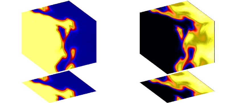
Figure 5: From left to right instantaneous mass fractions of H₂ and OH are shown. Unburnt turbulent gas in injected on the left.

For the test case shown here the turbulent intensity is 7 times larger than the laminar flame velocity $S_{\rm L}=10.2$ m s^-1. We find that for the mean inlet velocity $3S_{\rm L}$ the flame is nearly stationary inside the domain. This indicates that the turbulent flame velocity in this case is around $3S_{\rm L}$. However, it is hard to determine the turbulent flame speed precisely, because it is difficult to make the flame perfectly stationary inside the domain. This is partly because of the fact that between inlet and outlet the turbulence is decaying. Far from the inlet the turbulence is weaker than close to the inlet, whereas the turbulent flame speed increases with the turbulent intensity. As a result, the flame which is already far from the inlet tends to move even further downstream and the flame brush becomes broader.

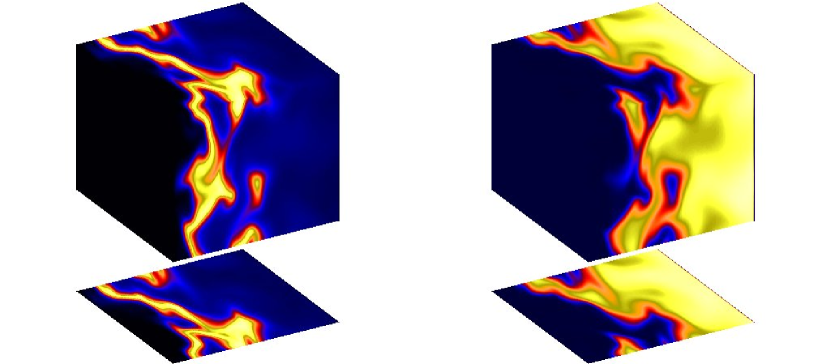
Figure 6: As Fig. 5, but for the instantaneous mass fraction of HO₂ on the left and temperature on the right.

In Fig. 5 one can see that the H₂ fuel (on the left hand side of the domain) is all consumed over the flame brush. The thickness of the flame brush is of the order of half the box length ($2.5$ mm) and is slightly smaller than the integral scale of the turbulence. The mass fraction of OH is shown in the right hand figure. It is clearly seen that OH does not burn out after the flame, but due to the very high temperatures downstream of the flame front the mass fraction of OH stays rather constant. For HO₂ the situation is however rather different and it exists only in the neighborhood of the reaction zone of the flame (see the left hand figure of Fig. 6). This indicates that HO₂ might be used as an indicator of the reaction zone. In the right-hand figure the temperature is shown to increase from 750 K to 1984 K, but the maximum value will increase even more downstream of the box due to radical reconnection.

In addition, we find that the turbulence is damped behind the flame front, and the burnt gas stream looks much more laminar there (not shown here). This happens because the values of temperature and hence also viscosity of the burnt gas are much larger than those of the unburned mixture.

5.1.1 Timings

As DNS is very CPU intensive, it is crucial that the timings are as good as possible. The current setup has been tested on a single processor with different chemistry and transport data, and the results are presented in Table 2. Run A, with the full Li mechanism and mixture averaged transport coefficients, use the most resources, as expected. By simplifying the transport data [21] (Run C) Eq. (17) is substituted by

$$D_{k}=D_{0}\frac{T^{n}}{\rho}$$ (33)

and Eq. (23) is substituted by

$$\lambda=\rho c_{p}\kappa_{0}T^{n}$$ (34)

where $n=0.7$ and $D_{0}=\kappa_{0}=2.9\times 10^{-5}$ g/(s cm Kⁿ) leading to a 28% reduction in CPU consumption. Lets now turn off reactions, but still keeping all the 13 species (Run D), and an additional 53% reduction is achieved.

For comparison, Run E is shown in order to see how much is gained by solving only the Navier-Stokes equation together with the continuity equation, assuming an isothermal medium with transport coefficients and thermodynamics such that all species can be neglected. It is seen that this is 20 times faster than Run D. This large difference is due to the fact that for Run E only 4 equations are solved, in contrast to the 18 equations for run D. Furthermore, and even more importantly, the time consuming process of determining the thermodynamics, such as enthalpy and heat capacity, together with the calculation of the viscosity, is omitted.

5.2 Spherical flame front

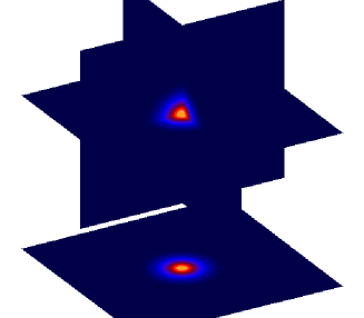
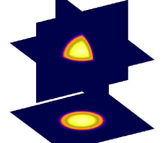
Figure 7: 3D images of the hot spot at moment $t=0$ s (left panel) and $t=1.2\times 10^{-4}$ s (right panel).

A study of the spherical and cylindrical flames is important because these cases are useful for determining important parameters in premixed combustion such as burning velocity, flame stretch rate, and flame curvature. There is a lot of numerical and experimental research in this area [13]. The most important difficulty in the numerical approach is the large computational demand. The typical mesh size has to be $\delta x=40-60$ $\mu$m [14], i.e. for a cube of 3 cm³ one needs about $500^{3}$ grid points and ideally 512 processors.

For illustration purposes we consider a smaller cube ($1\,{\rm cm}^{3}$), centered at the reference point with the hot spherical spot in its center (see Fig. 8). The initial hydrogen-air mixture with $Y_{\rm H_{2}}=2.4$ $\%$, $Y_{\rm O_{2}}=23$ $\%$ and $Y_{\rm N_{2}}=74.6$ $\%$ is under a pressure of $p=1$ bar. We use NSCBC boundary conditions, take a grid size of (80 $\times$ 80 $\times$ 80), and 25 processors on the Cray XT4/XT5. The results are presented in Figs. 7 and 8. The 3D images of the hot spot at the different moments (at $t=0$ s and $t=1.2\times 10^{-4}$ s) are presented in Fig. 7. In Fig. 8 one sees that the gas is burned in the center and then the flame front is expanding symmetrically in all three directions.

This problem is also used as a good test for the fully three dimensional NSCBC boundary conditions. We tested the implemented NSCBC boundary condition both for laminar and turbulent regimes. In the laminar case we find that due to the full NSCBC boundary conditions [18] the code runs well up to the moment when the flame front comes to the domain boundaries. In the turbulent regime the problems appear near the corners and edges of the domain because of the eddies at the boundaries. We avoid such a problem by using buffer (or sponge) zones (for details see [2]). We add the term to the right-hand side of the momentum equation

$$\frac{{\rm D}V_{i}^{j}}{{\rm D}t}=...-\frac{V_{i}^{j}-V_{{\rm ref},i}}{\tau}\zeta(x_{i}),\quad j=1,...,N_{i},$$ (35)

where $j$ denotes the meshpoint and $N_{i}$ is total number of grid points in the $i$ direction, and dots indicate the presence of terms that where already specified in equation (2), $\zeta(x_{i})$ is equal to zero everywhere except in the buffer zones where it is equal to unity. The length of the buffer zone is 10 $\%$ of the domain, and we choose $\tau=5\delta t$ and $V_{{\rm ref},i}=0$.

Figure 8: Temperature as a function of $x$ coordinate in the mid-plane of the box at $t=0$ s (dashed curve), $t=10^{-4}$ s (dotted-dashed curve) and $t=1.9\times 10^{-4}$ s (solid curve).

6 Conclusions

In this paper we have presented a high-order public domain code for direct numerical simulation of compressible flows with detailed chemical reactions. The Pencil Code provides sixth-order spatial accuracy in the simple one-step reaction case, and fifth order accuracy in the case where upwinding for density advection is necessary. For validation purposes we compare our results with the Chemkin tool for 0D and 1D test problems, and show that they are in good agreement. Finally, we calculate the flame speed in 3D both in laminar and turbulent cases.

The code is well suited for considering also more complicated reaction schemes such as methane combustion. Furthermore, it is straightforward to consider the interaction with additional chemicals such as nitrogen and to follow the production of NOx gases. In particular, it is important to consider combustion in the presence of steam. This is well known to lead to a reduction of NOx gases. Combustion in the presence of more complicated boundary conditions involving, for example, smaller inlet geometries has also been considered. Some of these cases, including those with a turbulent inlet, are available among the many sample cases that come with the code. For the benefit of the community, it is advantageous if prospective contributers to the code ask one of the code owners listed on http://pencil-code.googlecode.com/ to obtain permission as a committer.

$Header: /var/cvs/brandenb/f90/pencil-natalia/chemistry/tex/method/paper.tex,v 1.104 2010-05-28 11:53:45 nbabkovs Exp $

References

- The Pencil Code [2001] http://pencil-code.googlecode.com/.
- Babkovskaia et al. [2008] N. Babkovskaia, A. Brandenburg, J. Poutanen, J., Boundary layer on the surface of a neutron star, Monthly Notices Roy. Astron. Soc. 386 (2008) 1038–1044.
- Brandenburg [2001] A. Brandenburg, The inverse cascade and nonlinear alpha-effect in simulations of isotropic helical hydromagnetic turbulence, Astrophys. J. 550 (2001) 824–840.
- Brandenburg [2003] A. Brandenburg, Advances in nonlinear dynamos. The Fluid Mechanics of Astrophysics and Geophysics, Vol. 9 Eds. A. Ferriz-Mas & M. Núñez, Taylor & Francis, London and New York, 2003.
- Brandenburg & Dobler [2002] A. Brandenburg, W. Dobler, Hydromagnetic turbulence in computer simulations, Comp. Phys. Comm. 147 (2002) 471–475.
- CFX [2010] http://www.ansys.com/products/fluid-dynamics/cfx/
- Chemkin [2010] http://www.chemkin.com/
- Coffee & Heimerl [1981] T. P. Coffee, J. M. Heimerl, Transport algorithms for premixed, laminar steady-state flames, Combustion and Flame 43 (1981) 273–289.
- Doom et al. [2007] J. Doom, Y. Hou, K. Mahesh, A numerical method for DNS/LES of turbulent reacting flows, J. Comput. Phys. 226 (2007) 1136–115.
- Evlampiev [2007] Evlampiev, A.,PhD thesis, Technische Universiteit Eindhoven, 2007.
- Ferziger and Echekki [1993] J. H. Ferziger, T. Echekki, A simplified reaction rate model and its application to the analysis of premixed flames, Combust. Sci. Tech. 89 (1993) 293–351.
- Fluent [2010] http://www.fluent.com/
- Groot and De Goey [2002] G. Groot, L. De Goey, A computational study on propagating spherical and cylindrical premixed flames, Proceedings of the Combustion Institute, 29 (2002) 1445–1451
- Groot [2003] G. Groot, Model ling of propagating spherical and cylindrical premixed flames, PhD thesis, 2003.
- Gordon and McBride [1971] 1.S. Gordon, B. J. McBride, Computer Program for Calculation of Complex Chemical Equilibrium Compositions, Rocket Performance, Incident and Reflected Shocks and Chapman-Jouguet Detonations, NASA Report SP–273 (1971).
- Hirschfelder et al. [1969] J. O. Hirschfelder, J. O. Curtiss, R. B. Byrd, Molecular theory of gases and liquids, John Wiley & Sons, New York, 1969.
- Li et al. [2004] Li, J., Zhao, Z., Kazakov, A., Dryer, F. L., An updated comprehensive kinetic model of hydrogen combustion, Int. J. Chem. Kinet. 36 (2004) 566–575.
- Lodato et al. [2008] G. Lodato, P. Domingo, L. Vervisch, Three-dimensional boundary conditions for direct and large-eddy simulations of compressible viscous flows, J. Comput. Phys. 227 (2008) 5105–5143.
- OpenFOAM [2010] http://www.openfoam.com/
- Magnussen [1981] B. F. Magnussen, On the Structure of Turbulence and a Generalized Eddy Dissipation Concept for Chemical Reaction in Turbulent Flow, In Nineteenth AIAA Aerospace Meeting, St. Louis, 1981.
- Poludnenko and Oran [2010] A. Y. Poludnenko and E. S. Oran The interaction of high-speed turbulence with flames: Global properties and internal flame structure Combustion and Flame 157 (2010) 995–1011.
- Magnussen [1989] B. F. Magnussen, Modeling of Pollutant Formation in Gas Turbine Combustors Based on The Eddy Dissipation Concept, In Eighteenth International Congress on Combustion Engines, Tianjin, China, 1989.
- Magnussen and Hjertager [1976] B. F. Magnussen and B. H. Hjertager, On mathematical modeling of turbulent combustion with special emphasis on soot formation and combustion, In Sixteenth Symposium (International) on Combustion, The Combustion Institute, Pittsburgh, 1976, p. 719.
- Monchick and Mason [1961] L. Monchick, E. A. Mason, Transport properties of polar gases, J. Chem. Phys. 35 (1961) 1676–1697.
- Mourits and Rummens [1977] M. M. Mourits, F. H. A. Rummens, A critical evaluation of Lennard-Jones and Stockmayer potential parameters and of some correlation methods, Can. J. Chem. 55 (1977) 3007–3020.
- Poinsot and Lele [1992] T. Poinsot, S.K. Lele, Boundary conditions for direct simulations of compressible viscous flows, J. Comput. Phys. 101 (1992) 104–129.
- Poinsot and Veynante [2005] T. Poinsot, D. Veynante, Theoretical and Numerical Combustion, Edwards, 2005.
- Strohle and Myhrvold [2007] J. Strohle, T. Myhrvold, An evaluation of detailed reaction mechanism for hydrogen combustion under gas turbine conditions, 32 (2007) 125–135.
- Warnatz [1982] J. Warnatz, in Numerical Methods in Flame Propagation, edited by N.Peters and J. Wamatz Friedr. Vieweg and Sohn, Wiesbaden, 1982.
- Wilke [1950] C. R. Wilke, A Viscosity Equation for Gas Mixtures, J. Chem. Phys. 18 (1950) 517–519.
- Williams [1985] F. A. Williams, Combustion Theory, Benjamin Cummings, Menlo Park, CA, 1985.
- Williamson [1980] J. H. Williamson, Low-storage Runge-Kutta schemes, J. Comput. Phys. 35 (1980) 48–56.