Feshbach resonances of harmonically trapped atoms

Abstract

Employing a short-range two-channel description we derive an analytic model of atoms in isotropic and anisotropic harmonic traps at a Feshbach resonance. On this basis we obtain a new parameterization of the energy-dependent scattering length which differs from the one previously employed. We validate the model by comparison to full numerical calculations for ⁶Li-⁸⁷Rb and explain quantitatively the experimental observation of a resonance shift and trap-induced molecules in exited bands. Finally, we analyze the bound state admixture and Landau-Zener transition probabilities.

In the last decade reams of fascinating experiments with ultracold atoms have been carried out with applications ranging from studying condensed matter Hamiltonians and new phases of matter to performing quantum information processing Jaksch and Zoller (2005). Two key techniques made these achievements possible: (i) Atom-atom interaction characterized by the $s$-wave scattering length $a$ can be tuned using a magnetic Feshbach resonance (MFR). (ii) Atoms can be confined in various geometries such as dipole traps, optical lattices, or atomic waveguides Bloch et al. (2008). The known theory of MFR’s successfully describes the free scattering process for varying magnetic field $B$ and energy $E\rightarrow 0$. However, for the full understanding and precise controllability of confined atoms at an MFR a trap-version of this theory is needed which incorporates the energy dependence of the scattering process. This is especially the case for strong confinement which has been lately used to explore confinement-induced resonances and scattering in mixed dimensions Haller et al. (2010); *cold:lamp10. These systems show exciting behavior such as the formation of confinement-induced molecules Moritz et al. (2005).

In the following we present an approach to analytically describe MFR’s of harmonically trapped atoms. We obtain the eigenenergy equation, the admixture of the resonant molecular bound state $A(E,B)$, and a general parameterization of the energy-dependent scattering length $a(E,B)$. We show that the energy dependence of $a$ differs significantly from the one previously used to describe trapped gases Bolda et al. (2002); *cold:wout03; *cold:kryc09; Idziaszek and Calarco (2006) while it confirms the functional form of other two-channel models for trapped atoms Dunn et al. (2005); *cold:moor06; *cold:nyga08. We derive energy-dependent formulations of the resonance width and resonance shift and extend the model to anisotropic harmonic traps. The validity of our approach is verified by comparing to full multi-channel calculations for ⁶Li-⁸⁷Rb in harmonic confinement.

We demonstrate the usefulness of the new model by explaining the experimental observation of a shift of the resonance position of ⁸⁷Rb in an optical lattice Widera et al. (2004) and by circumstantiating the observation of confinement-induced molecules in exited states by Syassen et al. (2007). We analyze the bound state admixture and show that it might be responsible for enhanced losses of trapped ⁶Li far away from the resonance Bourdel et al. (2003). Finally, Landau-Zener transition probabilities are derived from the full energy spectrum.

Hamiltonian

We consider the relative-motion $s$-wave Hamiltonian of two atoms in harmonic confinement $\hat{H}=-\frac{\hbar^{2}}{2m}\frac{d^{2}}{dR^{2}}+\frac{1}{2}m\omega^{2}R^{2}+\hat{V}_{ZH}+\hat{V}_{\rm int}(R)$ with reduced mass $m$, trap frequency $\omega$, Zeeman and hyperfine energy $\hat{V}_{ZH}$, and the electron-spin dependent interaction potential $\hat{V}_{\rm int}(R)$. Within the two-channel (TC) description one projects onto the subspace of open and closed channels with the operators $\hat{\rm P}$ and $\hat{\rm Q}$, respectively. We consider the case of an elastic collision with one open channel. This results in the coupled equations

$$(\hat{\rm H}_{P}-E)|\Psi_{P}\rangle+\hat{\rm W}|\Psi_{Q}\rangle = 0\,,$$ (1)

$$(\hat{\rm H}_{Q}-E)|\Psi_{Q}\rangle+\hat{\rm W}^{\dagger}|\Psi_{P}\rangle = 0\,,$$ (2)

with $\hat{\rm H}_{P}=\hat{\rm P}\hat{\rm H}\hat{\rm P}$, $\hat{\rm H}_{Q}=\hat{\rm Q}\hat{\rm H}\hat{\rm Q}$, $\hat{\rm W}=\hat{\rm P}\hat{\rm H}\hat{\rm Q}$, $|\Psi_{P}\rangle=\hat{\rm P}|\Psi\rangle$, $|\Psi_{Q}\rangle=\hat{\rm Q}|\Psi\rangle$, and $E$ the energy above the threshold of the open-channel interaction potential Schneider and Saenz (2009). Furthermore, one assumes that close to the MFR $|\Psi_{Q}\rangle$ is simply a multiple $A$ of a bound eigenstate $|\Phi_{b}\rangle$ with eigenenergy $E_{b}$. We call this closed-channel state “resonant bound state” (RBS). To first order, the energy $E_{b}$ may be expanded linearly in the magnetic field $B$, i.e. $E_{b}(B)=\mu(B-B_{0})$.

Be $|\Phi_{E}\rangle$ the normalized solution of the open channel with $|\Psi_{P}\rangle=C|\Phi_{E}\rangle$ then $C^{2}+A^{2}=1$ holds which allows us to define a phase $\tan\delta_{\rm\scriptscriptstyle RBS}=A/C$ attributed to the RBS admixture. Introducing $|\Psi_{P}\rangle=C|\Phi_{E}\rangle$ and $|\Psi_{Q}\rangle=A|\Phi_{b}\rangle$ into Eq. (2) and multiplying by $\langle\Phi_{b}|$ gives

$$\tan{\delta_{\rm\scriptscriptstyle RBS}}=\frac{\langle\Phi_{E}|\hat{W}|\Phi_{b}\rangle}{(E-E_{b})}\,.$$ (3)

For infinite detuning $E-E_{b}$ the open channel is assumed to be in some background eigenstate $|\Phi_{\rm bg}\rangle$ of $\hat{\rm H}_{P}$ with eigenenergy $E_{\rm bg}$. Multiplying Eq. (1) by $|\Phi_{\rm bg}\rangle$ and using Eq. (3) yields the eigenenergy equation

$$(E-E_{b})(E-E_{\rm bg})=\frac{\langle\Phi_{\rm bg}|\hat{W}|\Phi_{b}\rangle\langle\Phi_{E}|\hat{W}|\Phi_{b}\rangle}{\langle\Phi_{\rm bg}|\Phi_{E}\rangle}\,.$$ (4)

Short-range approximation

In order to find simplified expressions for $\langle\Phi_{\rm bg}|\hat{W}|\Phi_{b}\rangle$, $\langle\Phi_{E}|\hat{W}|\Phi_{b}\rangle$, and $\langle\Phi_{\rm bg}|\Phi_{E}\rangle$ we assume that the interaction acts only in some small range $R<R_{\rm int}\ll a_{\rm ho}$ such that for $R>R_{\rm int}$ the solution $|\Phi_{E}\rangle$ is given by $\tilde{\Phi}_{E}(R)=A_{\nu}D_{\nu}(\rho)$, where $D_{\nu}(\rho)$ is the parabolic cylinder function, $\rho=\sqrt{2}R/a_{\rm ho}$, $a_{\rm ho}=\sqrt{\hbar/(m\omega)}$, $\nu=E/(\hbar\omega)-1/2$, and $A_{\nu}$ is a normalization constant. For $R\ll a_{\rm ho}$ one has $D_{\nu}(\rho)=D_{\nu}(0)\left(1-\rho/[\sqrt{2}f(E)]\right)$ with $f(E)=\Gamma\left(\frac{1}{4}-\frac{E}{2\hbar\omega}\right)/2\Gamma\left(\frac{3}{4}-\frac{E}{2\hbar\omega}\right)$ Abramowitz and Stegun (1965). Considering the logarithmic derivative one obtains the scattering length $a(E)=a_{\rm ho}f(E)$, which is equivalent to the result in Busch et al. (1998).

In the spirit of a Taylor expansion we parameterize $\langle\Phi_{E}|\hat{W}|\Phi_{b}\rangle$ by a linear combination $\alpha\,\tilde{\Phi}_{E}(0)+\beta\,\tilde{\Phi}_{E}^{\prime}(0)$. That is, one can define a $\gamma_{E}$ and an $a^{*}$ such that

$$\langle\Phi_{E}|\hat{W}|\Phi_{b}\rangle=\gamma_{E}\tilde{\Phi}_{E}(0)\left(1-\frac{a^{*}}{a}\right)\,.$$ (5)

Here, $\gamma_{E}$ describes the coupling strength to the RBS and $a^{*}$ defines the scattering length of the state $|\Phi_{E}\rangle$ when it is orthogonal to $\hat{W}|\Phi_{b}\rangle$. Since the orthogonality fixes the phase of $|\Phi_{E}\rangle$ within the coupling range the energy-dependence of $a^{*}$ should be usually negligible. We find that also the variation of $\gamma_{E}$ is negligible which can be explained by the stability of the nodal structure of $|\Phi_{E}\rangle$ for most of the coupling range. Analogous to Eq. (5), we set $\langle\Phi_{\rm bg}|\hat{W}|\Phi_{b}\rangle=\gamma_{\rm bg}\tilde{\Phi}_{E_{\rm bg}}(0)\left(1-\frac{a^{*}}{a_{\rm bg}}\right)$ where we allow for a different coupling strength $\gamma_{\rm bg}$ of the uncoupled background state to the RBS. We assume $a^{*}$ to have the same value as in Eq. (5) since it is determined by the requirement of orthogonality to the constant term $\hat{W}|\Phi_{b}\rangle$.

Finally, we set $\langle\Phi_{\rm bg}|\Phi_{E}\rangle=\langle\tilde{\Phi}_{\rm bg}|\tilde{\Phi}_{E}\rangle$ neglecting the behavior of the wave-functions at $R<R_{\rm int}$. This approximation cannot reproduce the exact energies $E$ where $\langle\Phi_{\rm bg}|\Phi_{E}\rangle=0$ that depend on the nodal structure at $R<R_{\rm int}$. However, it is applicable in a sufficient range around $E=E_{\rm bg}$ such that states of any energy can be described by choosing an appropriate background state.

Applying these assumptions to Eq. (4) and using the properties of $\langle D_{\nu}|D_{\nu^{\prime}}\rangle$ Gradshteyn and Ryzhik (2007) one finds the analytic eigenenergy equation

$$E-E_{b}=\frac{2\gamma_{\rm bg}\gamma_{E}}{a_{\rm ho}\hbar\omega}\frac{\left(f(E)-\frac{a^{*}}{a_{\rm ho}}\right)\left(f(E_{\rm bg})-\frac{a^{*}}{a_{\rm ho}}\right)}{f(E)-f(E_{\rm bg})}\,.$$ (6)

Energy-dependent scattering length

In order to determine the interaction dependent scattering length $a(E,B)$ we demand that it is equal to the scattering length $a_{\rm ho}f(E)$ of $\tilde{\Phi}_{E}(R)$, i.e. that the eigenenergies are given by the roots of $a(E,B)=a_{\rm ho}f(E)$. Since $R_{\rm int}\ll a_{\rm ho}$ the trap has no influence on the interaction and thus on $a(E,B)$. The value of $f(E_{\rm bg})$ in Eq. (6) is in analogy determined by the root of the eigenequation for the uncoupled problem $a_{\rm bg}(E_{\rm bg})=a_{\rm ho}f(E_{\rm bg})$ which is closest to $E$. Here, $a_{\rm bg}$ is the background scattering length that varies with the energy approximately like $a_{\rm bg}(k)^{-1}=a_{0}^{-1}-\frac{1}{2}k^{2}R_{\rm eff}$ with $k^{2}=2mE/\hbar^{2}$, $a_{0}$ the zero-energy background scattering length, and $R_{\rm eff}>0$ the effective range that can be well estimated from the van-der-Waals coefficient $C_{6}$ Flambaum et al. (1999). Since the interaction is trap independent one can use the $\omega\rightarrow 0$ limit to set $f(E_{\rm bg})\equiv a_{\rm bg}(E)/a_{\rm ho}$. Then, rearranging Eq. (6) yields

$$a(E,B)=a_{\rm bg}(E)\left(1-\frac{\Delta B}{B-B_{0}+\delta B-E/\mu}\right)$$ (7)

with resonance width $\Delta B=\frac{2\gamma_{\rm bg}\gamma_{E}ma_{\rm bg}}{\mu\hbar^{2}}\left(1-\frac{a^{*}}{a_{\rm bg}}\right)^{2}$ and detuning $\delta B=a_{\rm bg}\Delta B/(a_{\rm bg}-a^{*})$. The scattering length $a^{*}=a(E=0,B_{0})$ has an important impact on the behavior of $\Delta B$ and $\delta B$. For small $a_{\rm bg}/a^{*}$ one has $\Delta B\propto a_{\rm bg}^{-1}$ and $\delta B\approx$ const. while for systems with large $a_{\rm bg}$ the value of $a^{*}$ is negligible such that $\delta B=\Delta B\propto a_{\rm bg}$.

Let us compare the result to the previously used energy dependence of the scattering length given as Bolda et al. (2002); *cold:wout03; *cold:kryc09; Idziaszek and Calarco (2006)

$$a(E,B)=a_{\rm bg}\left(1-\frac{\Delta B\left(1+(ka_{\rm bg})^{2}\right)}{B-B_{0}+\delta B+(ka_{\rm bg})^{2}\Delta B-E/\mu}\right)\,.$$ (8)

Here, the term $(ka_{\rm bg})^{2}$ induces an additional energy-dependence. We examined a two-channel model system and found no energy dependence connected to $(ka_{\rm bg})^{2}$ while the behavior described by Eq. (7) could be validated . The absence of the dependence on $(ka_{\rm bg})^{2}$ is also supported by other two-channel models in the presence of a trapping potential Dunn et al. (2005); *cold:moor06; *cold:nyga08.

RBS admixture

From the formal limit $E_{\rm bg}\rightarrow E$ of Eq. (6) and of the short-range approximation of Eq. (4) one can infer that $\tilde{\Phi}_{E}^{2}(0)=\frac{2}{a_{\rm ho}\hbar\omega}\frac{f^{2}(E)}{f^{\prime}(E)}$. With this the short-range approximation of Eq. (3) can be written in terms of $f(E)$ as

$$\tan^{2}\delta_{\rm\scriptscriptstyle RBS}=\frac{\gamma_{E}}{\gamma_{\rm bg}}\frac{a_{\rm ho}}{a_{\rm bg}\mu\Delta B}\frac{\left(f(E)-a_{\rm bg}/a_{\rm ho}\right)^{2}}{f^{\prime}(E)}\,.$$ (9)

Extension to anisotropic harmonic traps

Our model can be easily extended to anisotropic harmonic traps. The eigenenergy relation in a trap with $\omega_{x}=\omega_{y}=\eta\omega_{z}$ is known to be $a=-\sqrt{\pi}d/\mathcal{F}(x,\eta)$ with $d,x,$ and $\mathcal{F}$ defined in Idziaszek and Calarco (2006). Since $a(E,B)$ is trap-independent we have to replace for $\eta\neq 1$ in the eigenenergy relation $a_{\rm ho}f(E)$ by $-\sqrt{\pi}d/\mathcal{F}(x,\eta)$. One can show that this necessitates the same replacement in the expression for $\tilde{\Phi}_{E}^{2}(0)$ and accordingly in Eq. (9).

Comparison with full numerical calculations

For the realistic case of ⁶Li-⁸⁷Rb we have performed full numerical multi-channel (MC) calculations in order to obtain eigenenergies and channel admixtures for different trap frequencies $\omega$ ($\eta=1$) and magnetic fields $B$. From the $E\rightarrow 0$ limit in free space we obtain $a_{0}=-17.77\,$a.u. and from the $C_{6}$ coefficient $R_{\rm eff}=1899.9\,$a.u. The magnetic field positions of vanishing and resonant scattering length and the channel admixtures at resonance of the first two trap states in a shallow trap with $\omega=2\pi\times 20\,$kHz yield the parameters $\mu=2.44\,\mu_{B}$, $a^{*}=63.14\,$a.u., $B_{0}=1064.62\,$G, $\gamma_{E}=2.73\times 10^{-8}\,$a.u., and $\gamma_{\rm bg}=2.63\times 10^{-8}\,$a.u.

Figure 1 shows a comparison of the eigenenergies and RBS admixture obtained from the full MC calculation and from our model in a trap with $\omega=2\pi\times 200\,$kHz which corresponds to a deep optical lattice. Both results are in very good agreement with a deviation $<0.003\,\hbar\omega$ and $<0.1\%$, respectively. This shows that the model accurately covers the $E$ and $B$ dependence of the scattering process. Only for energies well below zero, the model fails to reproduce $E$ and $A$ correctly. Here, the van-der-Waals interaction becomes dominant the long range such that the approximation of a short-rang interaction breaks down. For the considered trap the roles of $a^{*}$ and $a_{\rm bg}(E)$ become apparent through a significant broadening of $\Delta B$ by $0.18\,$G between the $1^{\rm st}$ and the $4^{\rm th}$ state.

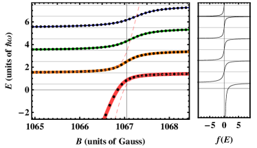
a)                                          b)
c)

Figure 1: a) Energy spectrum of ⁶Li-⁸⁷Rb as a function of the magnetic field $B$ in a trap with $\omega=2\pi\times 200\,$kHz. Dots indicate MC calculations while lines indicate solutions of Eq. (6). The eigenenergies of Eq. (11) are shown as dashed lines. b) Scattering length $a(E,B)/a_{\rm ho}=f(E)$ corresponding to an eigenenergy $E$ of the system. At $E=\hbar\omega(2n+1/2)$ with $n=\mathbb{N}$ resonances appear. c) Contribution $A^{2}$ of the RBS for each energy level as a function of the magnetic field $B$. Dots indicate MC calculations while lines indicate results of Eq. (9) with energies from solutions of Eq. (6).

Resonance position in the harmonic trap

As shown in Fig. 1 b) the resonances of the scattering length $a(E,B)\propto f(E)$ are located at $E_{\rm res}^{(n)}=\hbar\omega(2n+\frac{1}{2})$. In an anisotropic trap the resonance energies $E_{\rm res}^{(n)}$ are determined by the roots of $\mathcal{F}(x,\eta)$. Consequently, the magnetic resonance position changes according to Eq. (7) from the free-space position $B_{R}=B_{0}-\delta B$ to

$$B_{\rm res}^{(n)}=B_{0}-\delta B+E_{\rm res}^{(n)}/\mu\,.$$ (10)

The difference of the resonance position for each energy level $n$ opens the exciting possibility to tune the magnetic field to a resonance of a specific trap state which in turn enhances inelastic collisions depopulating this level. By successively adjusting the magnetic field at different resonance positions one might be able to engineer an ensemble in an excited state or cool the system to its relative-motion ground state. A good candidate for this approach would be an MFR of ¹³³Cs at $19.8\,$G where the small value of $\mu\Delta B=2\pi\times 4\,$kHz [See][andreferencestherein.]cold:chin10 admits to address single levels in reasonably deep traps.

Applying Eq. (10) one is able to explain the disagreement of an experimentally observed MFR position of ⁸⁷Rb in a negligibly weak trap ($B_{\rm res}=9.09(1)\,$G Erhard et al. (2004)) and a trap of frequency $\omega_{x}=2\pi\times 33\,$kHz, $\omega_{y}\approx\omega_{z}\approx 2\pi\times 42\,$kHz ($B_{\rm res}=9.121(9)\,$G Widera et al. (2004)). The energy dependence of $\delta B$ in unknown. However, its impact is likely to be negligible. For $C_{6}=4660\,$a.u. Klausen et al. (2001) it holds $\left.d\,\delta B/dE\right|_{E=0}<0.1\,\mu_{B}^{-1}$ for both $a_{\rm bg}\ll a^{*}$ and $a_{\rm bg}\gg a^{*}$ while $1/\mu=0.5\,\mu_{B}^{-1}$ [See][andreferencestherein.]cold:chin10. Hence, the resonance shift is approximately given by $E_{\rm res}^{(1)}/\mu=0.034\,$G which is in good agreement with the experimental results.

Trap-induced molecules in exited states

Another effect of the trap concerns the RBS admixture. It is present for each energy level [see Fig. 1 c)] which suggests that RBS molecules can be created not only in the bound state Partridge et al. (2005) but also in exited states, e.g. exited bands of an optical lattice. Indeed, these confinement-induced molecules have been experimentally observed by Syassen et al. (2007). By inducing Rabi oscillations between atoms and RBS molecules at a very narrow ⁸⁷Rb resonance ($\mu\Delta B=2\pi\times 2\,$kHz, $a_{\rm bg}=100.8\,$a.u.) they could produce a large number of molecules in an optical lattice with two atoms per site in the center. After a sudden change of the magnetic field they measured the number of unbound atoms featuring pronounced maxima and broad minima. The suppressed dissociation at the minima can be attributed to a strong RBS admixture of excited trap states. Supported by our MC calculations for ⁶Li-⁸⁷Rb we assume $\gamma_{E}\approx\gamma_{\rm bg}$ in order to estimate the RBS admixture using Eq. (9). Figure 2 shows the atom number observed in Syassen et al. (2007) and the RBS admixture for excited eigenstates at different magnetic fields. Clearly, a large RBS admixture coincides with suppressed dissociation. Here, the RBS molecules survive as part of an eigenstate of the new Hamiltonian while for magnetic fields where the RBS admixtures are small the projection of the RBS onto the eigenstates leads to a larger fraction of unbound atoms. The effects of the energy-dependence of $a_{\rm bg}$ can be studied by an effective range approximation $a_{\rm bg}=(a_{0}^{-1}-\frac{1}{2}k^{2}R_{\rm eff}+\frac{1}{4}k^{4}V_{\rm eff})^{-1}$. With $a_{0}=100.8\,$a.u., $R_{\rm eff}$ determined from $C_{6}=4660\,$a.u. Klausen et al. (2001) and $V_{\rm eff}=(1700\,{\rm a.u.})^{3}$ the positions of small RBS admixture are shifted towards those of maximal dissociation.

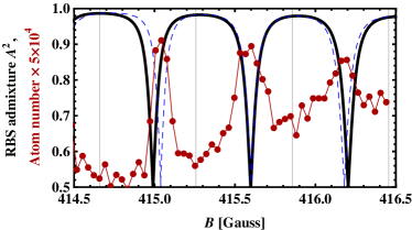
Figure 2: Atom number vs. magnetic field (dots) as measured in Syassen et al. (2007). RBS admixture of eigenstates according to Eq. (9) with $\gamma_{E}=\gamma_{\rm bg}$, $a^{*}\gg a_{\rm bg}$, and $a_{\rm bg}=a_{0}$ (solid line) and for an energy-dependent $a_{\rm bg}$ given in the text (dashed line).

Novel resonance phenomenon

For no external trap the resonance of the scattering length coincides with the maximal RBS admixture to the scattering wave function Schneider and Saenz (2009) such that the influence of both effects can hardly be distinguished. In traps this rule can be strongly violated. Searching for roots of the derivative of Eq. (9) with respect to $E$ one finds a maximal RBS admixture where $E$ solves $a_{\rm bg}(E)/a_{\rm ho}=f(E)-2f^{\prime}(E)^{2}/f^{\prime\prime}(E)$. For large $a_{\rm bg}$ and higher lying solutions $E_{\rm max}^{(n)}$ of this equation $E_{\rm max}^{(n)}$ can be far away from the resonance energies $E_{\rm res}^{(n)}$. Translated to the magnetic field the offset between the resonance position $B_{\rm res}^{(n)}$ and the position of maximal RBS admixture $B_{\rm max}^{(n)}$ can even approach $\Delta B$ which is accompanied by a vanishing scattering length at $B_{\rm max}^{(n)}$! Hence, this offset should be significant in a Fermionic system such as ⁶Li with a large background scattering length.

Bourdel et al. (2003) performed an experiment with $2N=7\times 10^{4}$ ⁶Li atoms in two different hyperfine states in a trap with $\omega_{x}=2\pi\times 0.78\,$kHz and $\omega_{y}\approx\omega_{z}\approx 2\pi\times 2.2\,$kHz Bourdel et al. (2003). They found a local maximum of atom loss close to $B_{R}$ but a global one at an about $-80\,$G shifted magnetic field. Atoms at the Fermi edge have a relative-motion energy equal to the Fermi energy $E_{F}=2\pi\hbar(6N\omega_{x}\omega_{y}\omega_{z})^{1/3}$. For $a_{0}=-1405\,$a.u., $\Delta B|_{E=0}=-300\,$G, $C_{6}=1393.4\,$a.u. [See][andreferencestherein.]cold:chin10 and $\eta=3$ our model predicts a maximal RBS admixture $-80.8\,$G shifted from the resonance. This agrees well with the maximum loss position which can be an indication that the RBS admixture enhances transitions to deeper bound states and thereby influences atom-loss processes. Note, that another qualitative explanation for the off-resonant loss has been given by Bourdel et al. (2003).

Landau-Zener avoided crossing

Finally, we derive Landau-Zener transition propabilities for each avoided crossing in the spectrum. Expanding $f(E)\approx f(E_{\rm bg})+f^{\prime}(E_{\rm bg})(E-E_{\rm bg})$ in Eq. (6) around some background energy $E_{\rm bg}$ yields the eigenenergy equation

$$(E-E_{b}-\mu\delta B)(E-E_{\rm bg})=\mu\Delta B\frac{f(E_{\rm bg})}{f^{\prime}(E_{\rm bg})}$$ (11)

which describes the avoided crossing of a molecular eigenstate to a background state with coupling strength $\delta^{2}=\mu\Delta Bf(E_{\rm bg})/f^{\prime}(E_{\rm bg})$. For the $n^{\rm th}$ avoided crossing and $a_{\rm bg}\ll a_{\rm ho}$ we have $1/f^{\prime}(E_{\rm bg})\approx 2\hbar\omega\binom{n-1/2}{n-1}/\sqrt{\pi}$ Busch et al. (1998) such that the diabatic transition probability is given as $P_{n}=e^{-2\pi G_{n}}$ with $G_{n}=|\delta^{2}/(\hbar\mu\dot{B})|\approx\left|2\omega\Delta Ba_{\rm bg}\binom{n-1/2}{n-1}/(\sqrt{\pi}a_{\rm ho}\dot{B})\right|$. Of course, only for $|\delta|\ll\hbar\omega$ the Landau-Zener theory can give exact results while otherwise two coupled states offer only a quantitative approximation. This can be judged from Fig. 1 a) for the first avoided crossing where $|\delta|\approx 1.4\hbar\omega$.

In conclusion, we developed an analytic model of atoms in isotropic and anisotropic harmonic traps experiencing a Feshbach resonance. The energy-dependent scattering length was determined and compared to a previous parameterization. Consequences of the model including a resonance shift, molecules in excited trap states, and a maximal molecular admixture away from the resonance were studied. Our model is in agreement with full numerical calculations and experimental results. We expect the approach to be applicable for an analytic treatment of other Feshbach-type resonances in a quasicontinuum.