Non-white frequency noise in spin torque oscillators and its effect on spectral linewidth

Abstract

We measure the power spectral density of frequency fluctuations in nanocontact spin torque oscillators over time scales up to 50 ms. We use a mixer to convert oscillator signals ranging from 10 GHz to 40 GHz into a band near 70 MHz before digitizing the time domain waveform. We analyze the waveform using both zero crossing time stamps and a sliding Fourier transform, discuss the different limitations and advantages of these two methods, and combine them to obtain a frequency noise spectrum spanning more than five decades of Fourier frequency $f$. For devices having a free layer consisting of either a single Ni${}_{\text{}80}$Fe${}_{\text{}20}$ layer or a Co/Ni multilayer we find a frequency noise spectrum that is white at large $f$ and varies as $1/f$ at small $f$. The crossover frequency ranges from $\approx 10^{4}\,\mathrm{Hz}$ to $\approx 10^{6}\,\mathrm{Hz}$ and the $1/f$ component is stronger in the multilayer devices. Through actual and simulated spectrum analyzer measurements, we show that $1/f$ frequency noise causes both broadening and a change in shape of the oscillator’s spectral line as measurement time increases. Our results indicate that the long term stability of spin torque oscillators cannot be accurately predicted from models based on thermal (white) noise sources.

I Introduction

In a spin torque oscillator (STO), a direct current passing through a reference magnetic layer becomes spin-polarized and transfers angular momentum to a second magnetic layer that is excited into steady-state oscillation. The oscillating magnetization causes an oscillating device resistance, through either the giant magnetoresistance effect or the tunneling magnetoresistance effect, which in combination with the bias current generates an oscillating voltage as the output signal. Interest in potential applications of STOs in integrated microwave circuits is driven by their rapid frequency tunability, small size ($\lesssim 100\,\mathrm{nm})$, and compatibility with standard semiconductor processing techniques. Recent reviews cover both the physics Ralph:2008pr and possible applications Silva:2008xd ; Katine:2008sh of STOs and other devices based on spin torque effects.

For any oscillator, noise is both an important figure of merit for applications and a useful probe of internal physical processes. Previous models of STO noise Tiberkevich:2007fc ; Kim:2008kx ; Kim:2008zr ; Tiberkevich:2008ys ; Kudo:2009fk ; SilvaKeller_preprint2010 have considered noise driven by a thermal source having a white power spectral density (PSD). Perhaps because most experiments on STOs have used a spectrum analyzer (SA) to measure signals in the frequency domain, most previous theoretical work has focused on how frequency noise determines the width of the spectral line. For purely white frequency noise, the relation is straightforward: a constant PSD $S_{\textrm{wh}}$ gives a Lorentzian spectral line whose full width at half maximum is simply $\Delta\nu_{\textrm{wh}}=\pi S_{\textrm{wh}}$ Lesage:1979dq ; Lax:1967cr . The situation is more complicated when the frequency noise is not white. Colored noise in STOs can occur both at high frequencies, due to an intrinsic relaxation rate that suppresses rapid frequency fluctuations Tiberkevich:2008ys ; SilvaKeller_preprint2010 , and at low frequencies as we demonstrate here. The stability of an oscillator cannot be described by a single number such as linewidth when its frequency noise is colored, and a measurement of the noise spectrum is required to accurately predict oscillator performance in specific applications and to test models of the physical origin of the noise.

In the next section we present generic equations for an oscillator in the time domain and introduce the various PSDs we use here. Then we describe our STO devices and our measurement techniques, including the use of a mixer to facilitate the measurement of signals well above 10 GHz. Next we describe two methods (both employing standard digital signal processing techniques) for computing the PSD of frequency fluctuations from the voltage waveform of the STO. While each method has different bandwidth limitations, when combined they yield noise spectra extending over more than five decades of Fourier frequency $f$. We present these combined spectra for two types of STOs, both of which show $1/f$ frequency noise below $f\approx 1\,\mathrm{MHz}$. Finally, we connect the frequency noise with SA measurements. The measured linewidth is larger than the value implied by the white part of the frequency noise spectrum and it increases with measurement time, effects that have been seen in semiconductor lasers having $1/f$ frequency noise. The line shape also changes, becoming more Gaussian at long measurement times, and we discuss how this affects the interpretation of STO line shape measurements.

II Time Domain Oscillator Model

The voltage output of a generic oscillator can be written as

$$V(t)=\left[{V_{0}+\epsilon(t)}\right]\sin\left[{2\pi\nu_{0}t+\phi(t)}\right],$$ (1)

where $\epsilon(t)$ is the deviation from the nominal amplitude $V_{0}$, $\nu_{0}$ is the nominal frequency, and $\phi(t)$ is the deviation from the nominal phase $2\pi\nu_{0}t$. From the total phase

$$\theta(t)\equiv 2\pi\nu_{0}t+\phi(t)$$ (2)

we define an instantaneous frequency

$$\nu(t)\equiv\frac{1}{2\pi}\frac{d\theta}{dt}=\nu_{0}+\frac{1}{2\pi}\frac{d\phi}{dt}.$$ (3)

From this equation, it is clear that phase and frequency are equivalent, not independent, ways of representing oscillator fluctuations.

Oscillator noise is commonly expressed in terms of the PSD of $V(t)$, $\phi(t)$, or $\nu(t)$, which we denote as $S_{V}(\nu)\;\mathrm{[V^{2}/Hz]}$, $S_{\mathrm{\phi}}(f)\;\mathrm{[rad^{2}/Hz]}$, and $S_{\nu}(f)\;\mathrm{[Hz^{2}/Hz]}$. The units of each PSD are given in square brackets and $f$ is Fourier frequency. Note that $S_{V}(\nu)$, the quantity measured by an SA with swept frequency $\nu$, includes amplitude noise that does not appear in the other two PSDs. These PSDs can be measured in various ways; we will describe the methods we use below. We will also make use of the Fourier identity

$$S_{\nu}(f)=f^{2}S_{\phi}(f),$$ (4)

which follows from the fact that frequency is the time derivative of phase.

III Experimental Methods

Our nanocontact STOs consist of a laterally extended spin valve structure and a metallic contact of nominal diameter 60 nm to 70 nm. Figure 1 shows the two types of structures we used. Both structures have a thick layer of Co${}_{\text{}90}$Fe${}_{\text{}10}$ that serves as the reference layer. We use “NiFe” to label devices whose free layer consists of $5\,\mathrm{nm}$ of Ni${}_{\text{}80}$Fe${}_{\text{}20}$ and “Co/Ni” to label devices whose free layer consists of a multilayer of Co and Ni. With no applied magnetic field, the free layer magnetization of the NiFe devices lies in the film plane, whereas that of the Co/Ni devices lies perpendicular to the film plane due to interfacial anisotropies intrinsic to the multilayer Daalderop:1992dp . The NiFe devices are from the same wafer as those used in Pufall:2007hb and the Co/Ni devices are from the same wafer as those used in Rippard:2010uq .

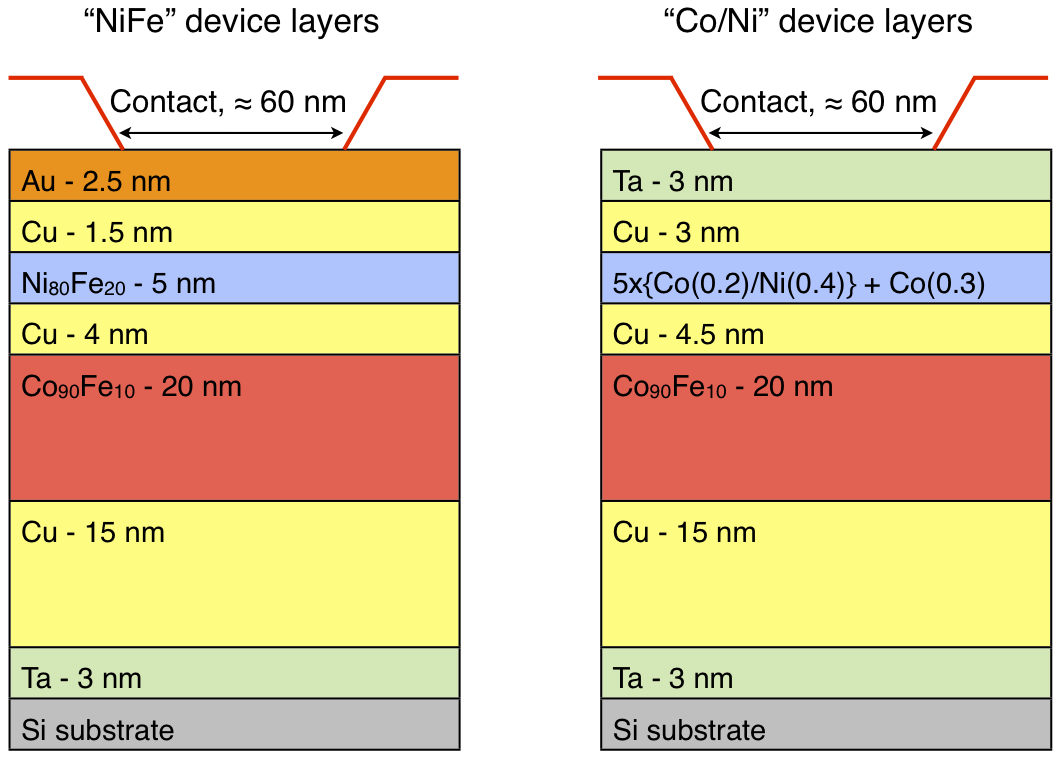
Figure 1: (Color online) Spin valve layers used for the NiFe and Co/Ni STO nanocontact devices. In each case, the layers extend laterally over a mesa of several $\mu\textrm{m}$ on a side. The current that generates the spin torque effect flows through a metallic nanocontact to the top layer and returns through the bottom Cu layer.

We used microwave probes to contact the devices, which were at room temperature. The high-frequency STO output, after separation from the bias current by a bias tee, passed through an amplifier with a power gain of 36 dB before entering an SA. We measured more than a dozen devices from four different wafers, at a variety of applied magnetic fields and bias currents, and we observed non-white frequency noise in all cases. Here we present representative data from one NiFe device and one Co/Ni device. The NiFe device was measured with a magnetic field $\mu_{0}H_{0}=1.0\,\mathrm{T}$ applied at an angle of $80^{\circ}$ from the film plane and a bias current $I_{\textrm{b}}=12.1\,\mathrm{mA}$, for which $\nu_{0}=13.2\,\mathrm{GHz}$. The Co/Ni device was measured with $\mu_{0}H_{0}=1.2\,\mathrm{T}$ applied at $85^{\circ}$ from the film plane and $I_{\textrm{b}}=7.5\,\mathrm{mA}$, for which $\nu_{0}=36.5\,\mathrm{GHz}$. We chose these conditions to illustrate how devices with nearly the same SA linewidth ($\approx 11\,\mathrm{MHz}$ in this case) can have significantly different frequency noise spectra.

Our technique for time domain measurements was motivated by a desire to measure STO signals well above 10 GHz using readily available commercial instruments. We used the intermediate frequency (IF) output of the mixer in an SA, with a fixed local oscillator (LO) frequency, to translate the input signal $V(t)$ to an IF signal $V_{\textrm{IF}}(t)$ centered at $70\,\mathrm{MHz}$. Ignoring the negligible phase noise of the LO, a perfect sine wave $V(t)$ would appear at the IF output as a perfect $70\,\mathrm{MHz}$ sine wave, whereas the frequency or phase fluctuations in an actual $V(t)$ appear as corresponding fluctuations in $V_{\textrm{IF}}(t)$. The advantage of the IF measurement technique is that STO signals for any $\nu_{0}$ within the range of the SA are translated to a common, lower frequency at which digitization is straightforward. A disadvantage is that the limited IF bandwidth prevents the measurement of signals with large linewidths. For the data presented here, the available IF band was approximately $(70\pm 20)\,\mathrm{MHz}$ and we were limited to STO signals with linewidths $\lesssim 30\,\mathrm{MHz}$. We used an oscilloscope to digitize $V_{\textrm{IF}}(t)$ at $10^{9}$ samples per second and to apply a digital $150\,\mathrm{MHz}$ lowpass filter to reduce preamplifier and oscilloscope noise. Figure 2 shows a portion of the resulting waveform. The available oscilloscope memory limited the duration of each filtered waveform to $\leq 50\,\mathrm{ms}$.

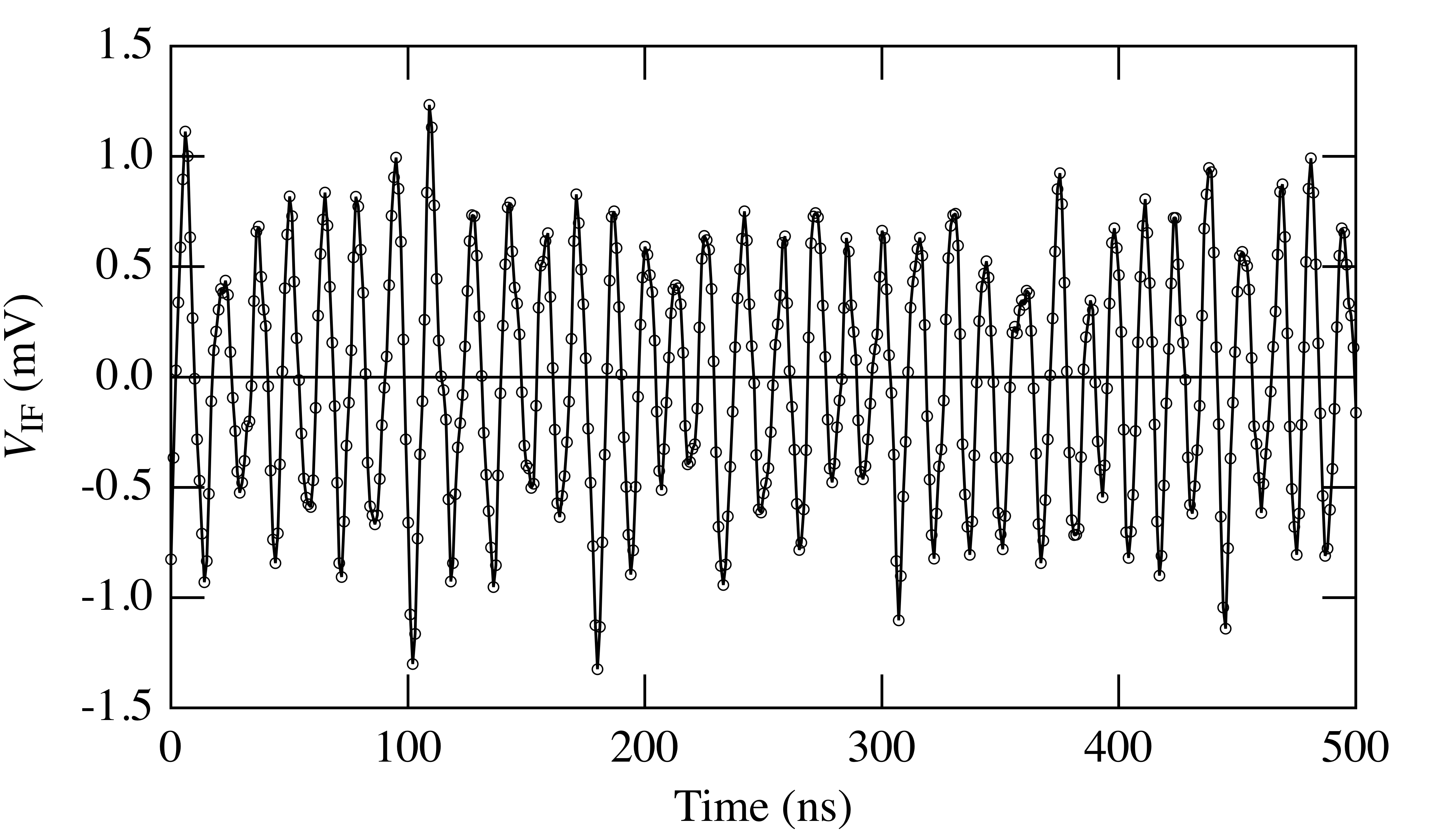
Figure 2: A short section of the IF waveform $V_{\textrm{IF}}(t)$ for the NiFe device. The amplitude variations seen in these data are dominated by amplifier noise.

IV Data Analysis Methods

In this section we describe two different methods for obtaining $S_{\nu}(f)$ from $V_{\textrm{IF}}(t)$. We discuss limitations and averaging considerations in some detail and we show that the two methods agree over their common range of $f$. Beyond the points we highlight here, many textbooks and other sources (e.g., Press:2007ek ) contain details of the digital signal processing techniques involved. In the next section we present composite spectra obtained by combining the two methods in order to cover a broader range of $f$ than is possible with either method alone while preserving the benefits of averaging.

The first analysis method is the “zero crossing” method. As described in Keller:2009ey , we obtain a value of the oscillator phase each time $V_{\textrm{IF}}(t)$ crosses zero, which yields $\phi(t)$ as shown in Figs. 3(a) and 3(b) for the NiFe device. Because the values of $\phi$ are not equally spaced in time, one should in principle estimate the PSD using an algorithm such as the Lomb periodogram Press:2007ek that is suitable for a time series with irregular spacing. However, in practice the variations in spacing are sufficiently small that we find no significant difference between the Lomb PSD and that obtained by assuming uniform spacing and applying conventional PSD algorithms. Thus for the analysis presented here we have replaced the actual time stamps in each $\phi(t)$ trace with values separated by the mean spacing for that trace. To reduce scatter in the spectra Press:2007ek , we averaged PSDs computed from half-overlapping segments of $\phi(t)$, each multiplied by a Hann window, to obtain $S_{\mathrm{\phi}}(f)$ shown in Fig. 3(c). We chose segment lengths of $1\,\mathrm{ms}$ and $10\,\mathrm{ms}$ to balance the tradeoff between averaging and frequency resolution. We found it necessary to omit the lowest three frequency bins from $S_{\mathrm{\phi}}(f)$ to obtain results that are independent of segment length; thus for $10\,\mathrm{ms}$ segments $S_{\mathrm{\phi}}(f)$ begins at $f=400\,\mathrm{Hz}$ rather than $(10\,\mathrm{ms})^{-1}=100\,\mathrm{Hz}$. (Spurious effects arise when there is a large difference between the initial and final values of $\phi$ for a segment. Consider a segment where $\phi(t)$ varies linearly: multiplying a line by a window that falls to zero at each end will create artificially large Fourier components near the inverse segment length.) Finally, we use Eq. (4) to obtain $S_{\mathrm{\nu}}(f)$ for the zero crossing method, with the result shown in Figure 3(d).

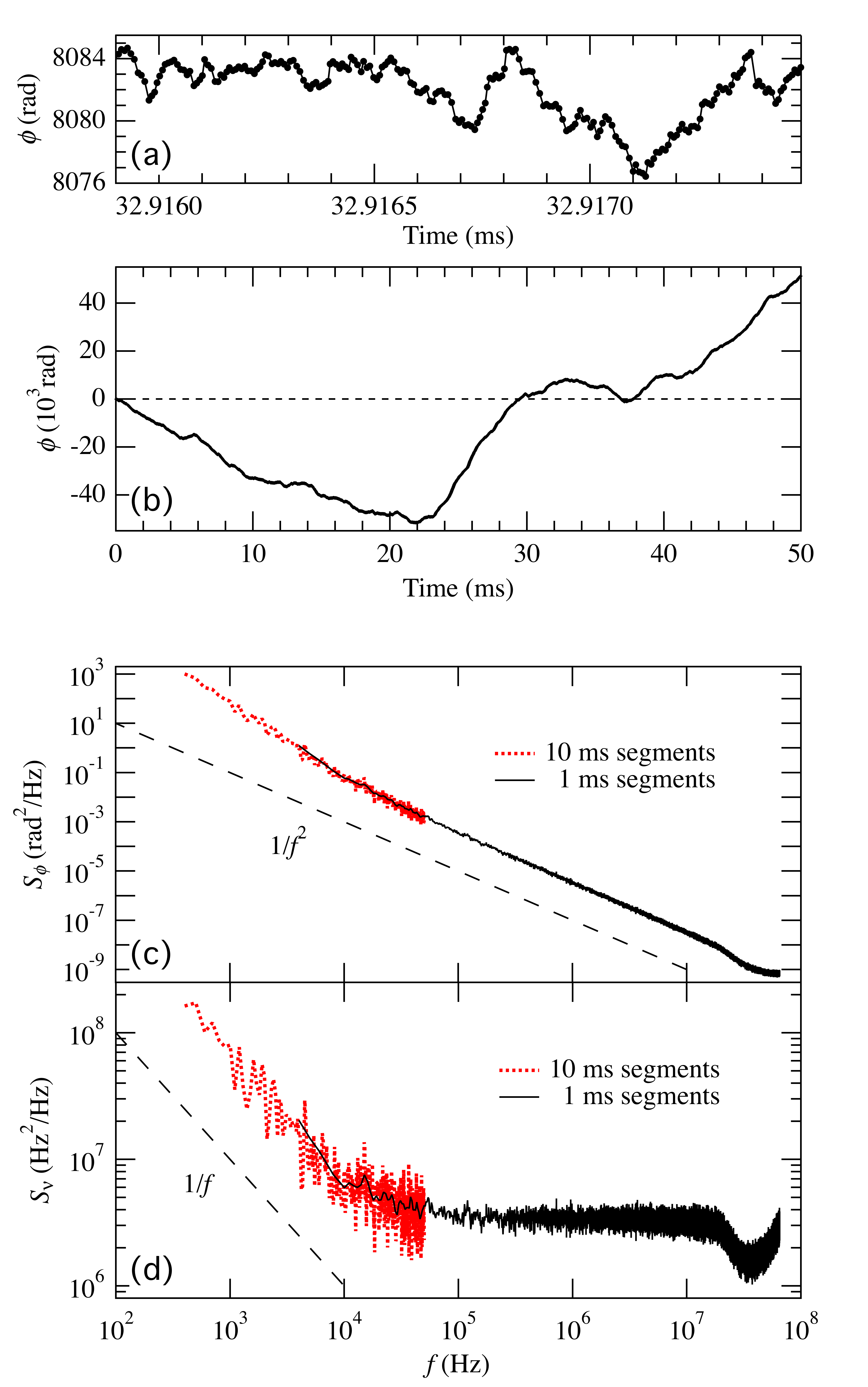
Figure 3: (Color online) Zero crossing method for computing $S_{\mathrm{\nu}}(f)$ from $V_{\textrm{IF}}(t)$. (a) Short section of $\phi(t)$ from zero crossings of $V_{\textrm{IF}}(t)$ for the NiFe device. (b) $\phi(t)$ for the entire $50\,\mathrm{ms}$ IF waveform. (c) Average $S_{\mathrm{\phi}}(f)$ computed from segments of $\phi(t)$ to reduce scatter in the PSD. (d) $S_{\mathrm{\nu}}(f)$ computed using Eq. (4). For both (c) and (d), dotted curves are the average PSD from 9 half-overlapping, $10\,\mathrm{ms}$ segments (points for $f>5\times 10^{4}\,\mathrm{Hz}$ are not shown) and solid curves are the average PSD from 99 half-overlapping, $1\,\mathrm{ms}$ segments. $S_{\mathrm{\phi}}(f)$ flattens near $10^{-9}\,\mathrm{rad{}^{2}/Hz}$ due to the noise floor for the zero crossing method set by amplifier noise in our setup Keller:2009ey , which causes the upturn in $S_{\mathrm{\nu}}(f)$ at large $f$. Dashed lines are visual guides indicating $1/f^{2}$ and $1/f$ power law spectra.

The rolloff in $S_{\mathrm{\nu}}(f)$ beginning at $f\approx 20\,\mathrm{MHz}$ qualitatively resembles the expected rolloff due to the intrinsic relaxation rate at which an STO returns to its stable precessional orbit after a fluctuation SilvaKeller_preprint2010 . However, in our case this rolloff is due to the limited bandwidth of the IF output (it occurs near $20\,\mathrm{MHz}$ in all our data) and does not reflect an intrinsic time scale of the STO. For the rest of this paper we show $S_{\mathrm{\nu}}(f)$ from the zero crossing method only for $f\leq 20\,\mathrm{MHz}$.

The second analysis method is the “sliding DFT” method. We compute the discrete Fourier transform (DFT) of half-overlapping segments of $V_{\textrm{IF}}(t)$ and fit a Lorentzian peak to the DFT to determine the center frequency for each segment . This yields a trace of $\nu(t)$, as shown in Figs. 4(a) and 4(b) for the NiFe device. The shortest segment that gave reliable results was $300\,\mathrm{ns}$, which for half-overlapping segments gives a value of $\nu$ every $150\,\mathrm{ns}$. We then compute $S_{\mathrm{\nu}}(f)$ for the DFT method from $\nu(t)$, again averaging the PSDs of half-overlapping, Hann-windowed segments. Since the relative excursions in $\nu(t)$ are much smaller than those in $\phi(t)$, there are no spurious effects for long segments and $S_{\mathrm{\nu}}(f)$ is independent of segment length over the entire range of $f$. We could easily obtain $S_{\mathrm{\phi}}(f)$ for the DFT method using Eq. (4), but the features of interest here are more easily seen in $S_{\mathrm{\nu}}(f)$.

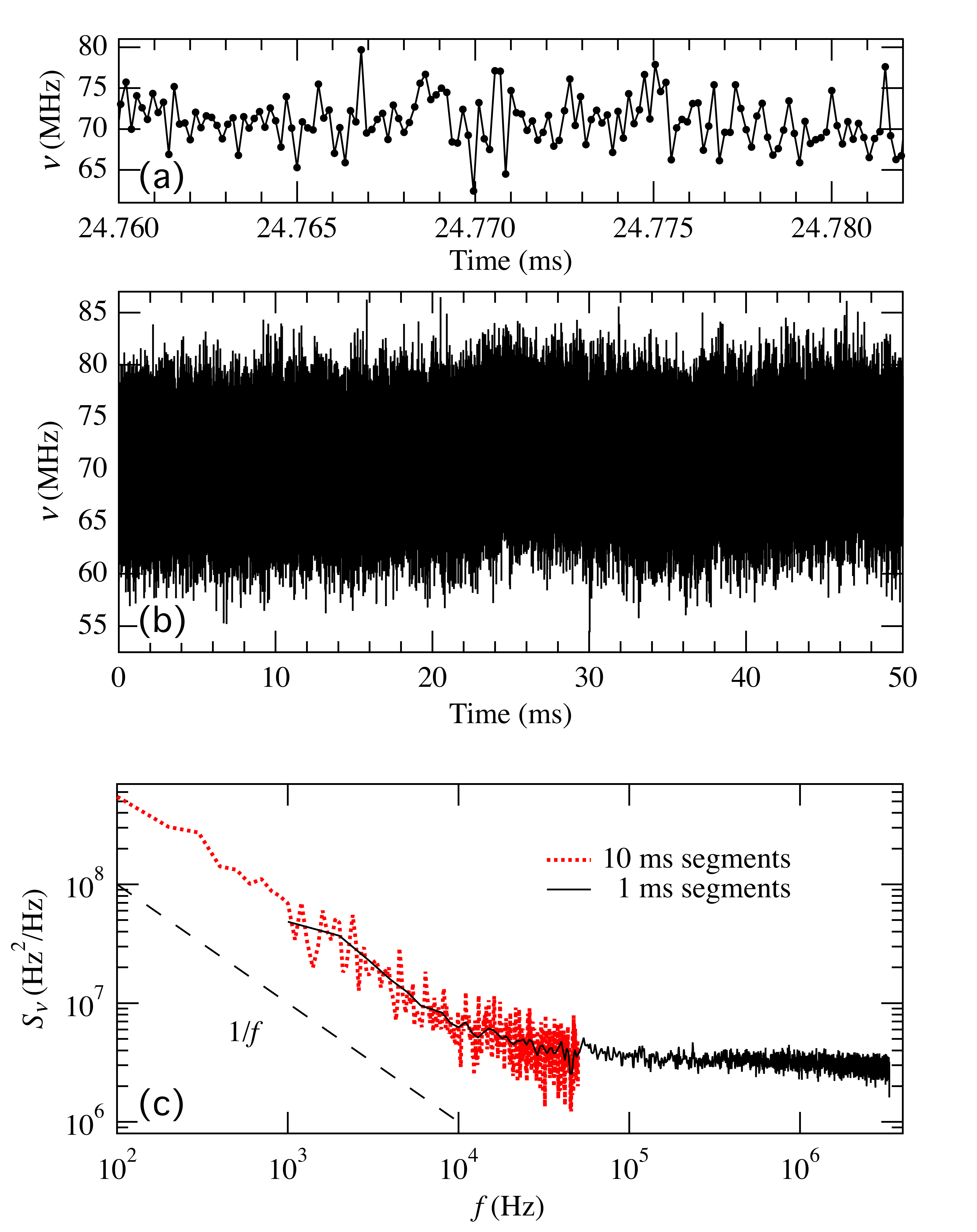
Figure 4: (Color online) Sliding DFT method for computing $S_{\mathrm{\nu}}(f)$ from $V_{\textrm{IF}}(t)$. (a) Short section of $\nu(t)$ from DFTs of half-overlapping segments of $V_{\textrm{IF}}(t)$ for the NiFe device. (b) $\nu(t)$ for the entire $50\,\mathrm{ms}$ IF waveform. (c) Average $S_{\mathrm{\nu}}(f)$ computed from segments of $\nu(t)$ to reduce scatter in the PSD. Dotted curve is for 9 half-overlapping, $10\,\mathrm{ms}$ segments (points for $f>5\times 10^{4}\,\mathrm{Hz}$ are not shown). Solid curve is for 99 half-overlapping, $1\,\mathrm{ms}$ segments. Dashed line is a visual guide indicating a $1/f$ power law spectrum.

In Fig. 5 we compare the average $S_{\mathrm{\nu}}(f)$ for $10\,\mathrm{ms}$ segments obtained from the two analysis methods. The two methods give nearly identical results over their common frequency range. Such agreement between two different routes to the same quantity is evidence that neither method is distorted by numerical artifacts, and thus that both methods reveal the actual frequency fluctuations of the oscillator . Comparing frequency ranges in Fig. 5, the zero crossing method extends up to $f=20\,\mathrm{MHz}$, while the DFT method is limited to $f\lesssim 3\,\mathrm{MHz}$ by the minimum DFT segment length mentioned above. On the other hand, since the DFT method avoids the spurious effects related to segment length, it extends to lower frequencies than the zero crossing method (for a given segment length).

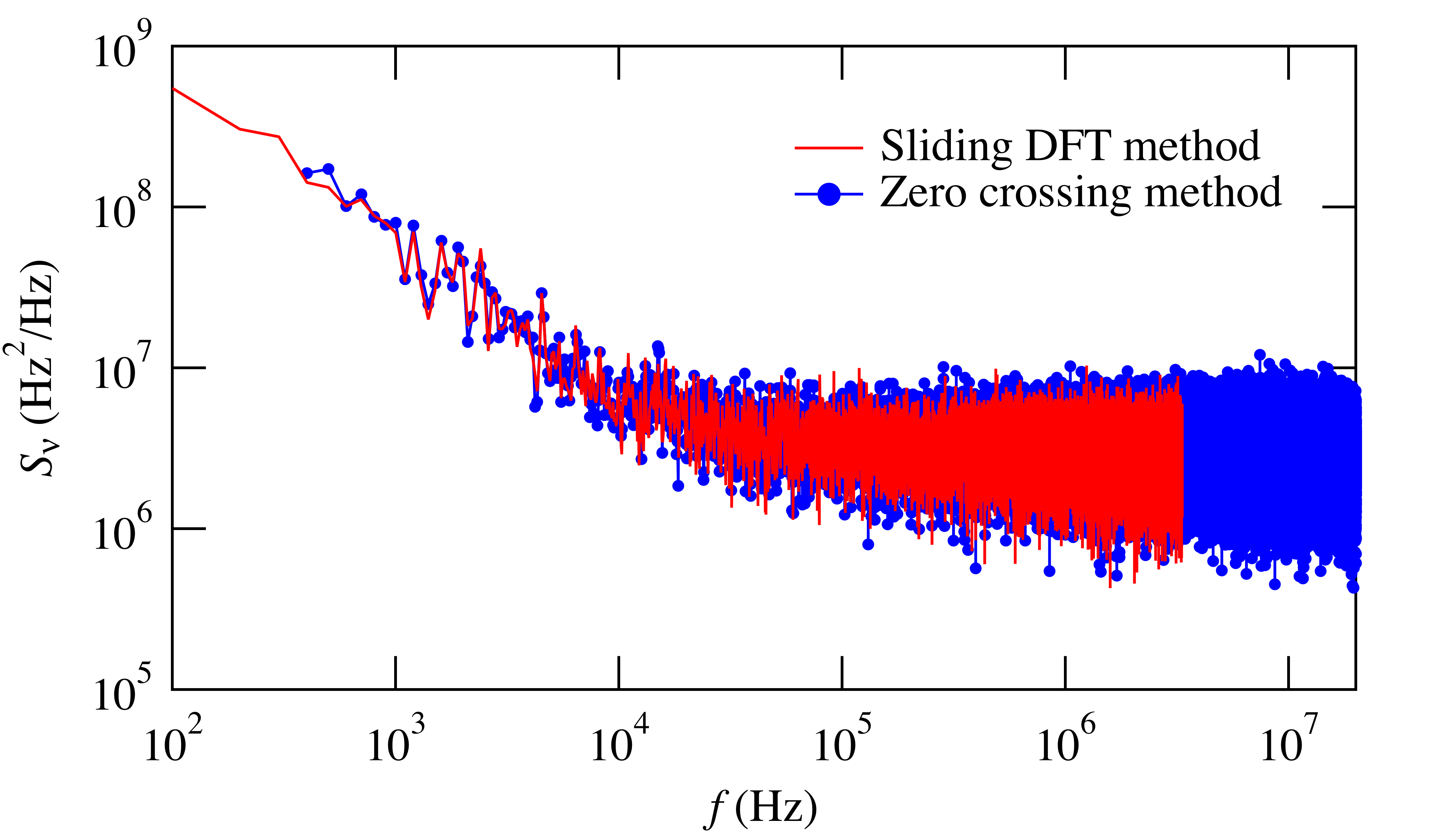
Figure 5: (Color online) Comparison of $S_{\mathrm{\nu}}(f)$ from two analysis methods for the NiFe device. The curves are those for $10\,\mathrm{ms}$ segments shown in Figures 3(d) and 4(c), here shown for all $f\leq 20\,\mathrm{MHz}$. The agreement indicates that numerical artifacts are likely negligible in both methods.

V Results and Discussion

As mentioned above, we combine spectra from the zero crossing and DFT methods to obtain $S_{\mathrm{\nu}}(f)$ over a larger frequency range than is possible with either method alone. As shown in Fig. 6, the zero crossing method using $1\,\mathrm{ms}$ segments together with the DFT method using $10\,\mathrm{ms}$ segments yields $S_{\mathrm{\nu}}(f)$ spanning more than five decades in $f$. Both the NiFe and Co/Ni devices show the same overall behavior: $S_{\mathrm{\nu}}(f)$ is constant at large $f$ (excluding the rolloff and noise floor features mentioned above) and varies as approximately $1/f$ at small $f$. We found this same qualitative behavior in all STOs we measured. For a given device, we have not found a clear dependence of either the white or $1/f$ noise on bias current or applied field, but our measurements to date have consisted of a broad survey rather than a search for systematic trends. One clear pattern that does emerge from our data is that the Co/Ni devices have stronger $1/f$ noise than the NiFe devices, as illustrated by the representative spectra in Fig. 6. The white noise for the two device types is typically comparable (factor of 2.5 difference in Fig. 6), while the $1/f$ component is typically 10 times larger in the Co/Ni devices (factor of 15 difference in Fig. 6). Whether this systematic difference is due to the different materials in the STO free layer, the different magnetic anisotropies (which lead to different precessional trajectories), or to other factors is an important topic for future investigations.

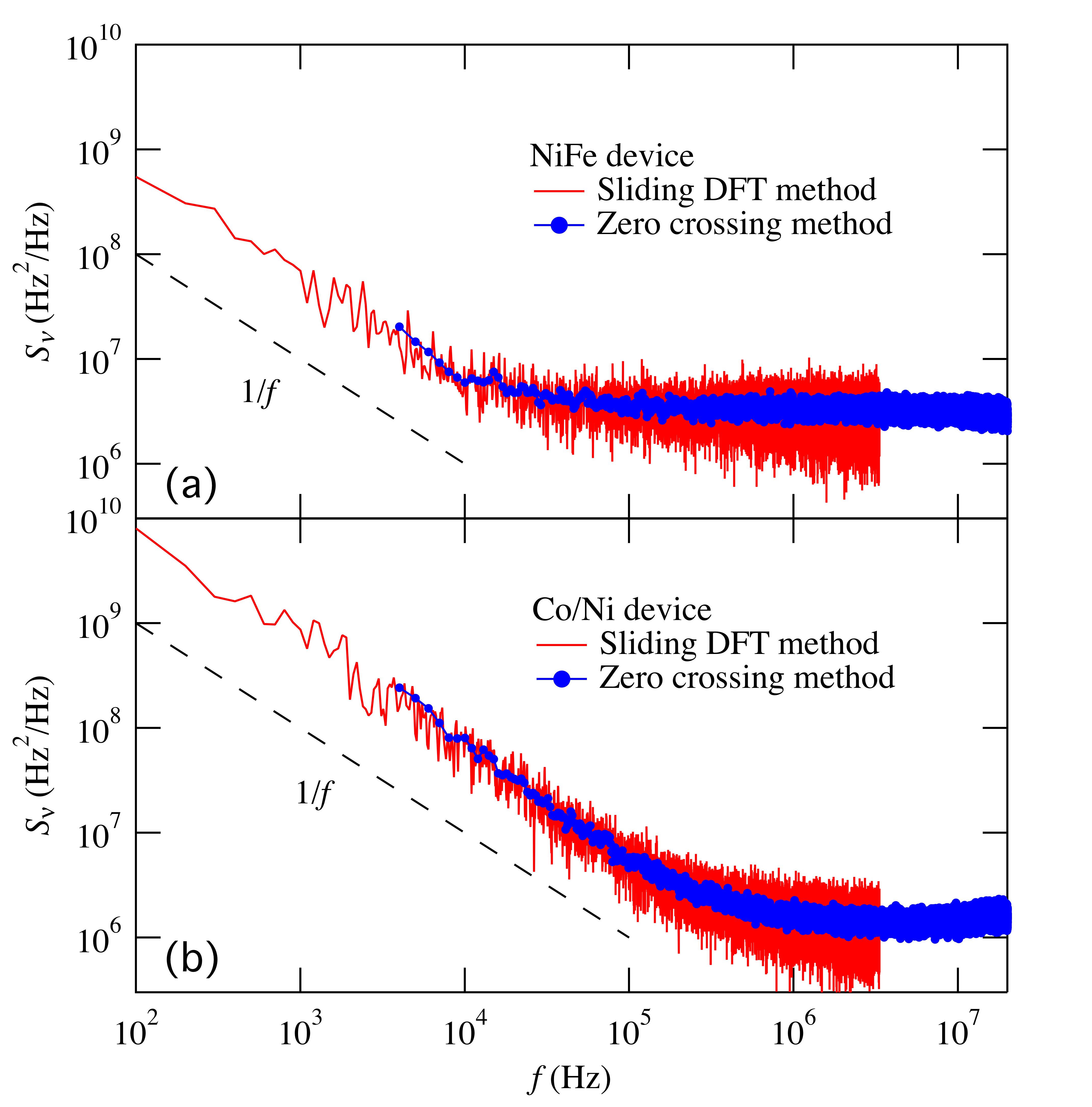
Figure 6: (Color online) Combined frequency noise from both analysis methods for (a) NiFe device and (b) Co/Ni device. Segment length is $1\,\mathrm{ms}$ for the zero crossing method and $10\,\mathrm{ms}$ for the sliding DFT method. Dashed lines are visual guides indicating a $1/f$ power law spectrum.

Several considerations rule out sources for the $1/f$ noise other than the STO itself. Noise from the bias current source is filtered by the dc path of the bias tee, which has a bandwidth of $8\,\mathrm{kHz}$, whereas we observed $1/f$ noise up to much higher frequencies. Furthermore, an effect due to bias current noise would scale with $|d\nu_{0}/dI_{\textrm{b}}|$ of the STO, but the devices shown in Fig. 6 follow the opposite trend: the NiFe device has a larger $d\nu_{0}/dI_{\textrm{b}}$ (by a factor of $\approx 3$) but weaker $1/f$ noise than the Co/Ni device. Noise from other sources such as the oscilloscope, preamplifier, or stray magnetic fields would affect all our measurements equally, which is not consistent with the reproducible differences among devices that we observed.

Another trend emerges when we compare the measured SA linewidth, $\Delta\nu_{\textrm{SA}}$, with the value expected from the white noise level in $S_{\mathrm{\nu}}(f)$, $\Delta\nu_{\textrm{wh}}$. (At this point we report Lorentzian linewidths for a measurement time of $1\,\mathrm{s}$; see below for why it is important to specify both line shape and time scale.) Our NiFe devices have SA linewidths that are 1.1 to 1.3 times larger than expected from the white noise: $\Delta\nu_{\textrm{SA}}=11.2\,\mathrm{MHz}$ and $\Delta\nu_{\textrm{wh}}=10.4\,\mathrm{MHz}$ for the device in Fig. 6 (all values of $\Delta\nu$ here have an uncertainty of approximately $\pm 0.5\,\mathrm{MHz}$ unless error bars on a plot indicate otherwise). In constrast, our Co/Ni devices have SA linewidths that are 2 to 3 times larger than expected from the white noise: $\Delta\nu_{\textrm{SA}}=10.0\,\mathrm{MHz}$ and $\Delta\nu_{\textrm{wh}}=4.1\,\mathrm{MHz}$ for the device in Fig. 6. As we describe next, this trend can be understood as a consequence of the different $1/f$ noise strength in the different devices.

Spectral line broadening due to $1/f$ frequency noise is well known in the field of single-mode semiconductor lasers. We first give a brief description of the key concepts and then apply them to our measurements in the next paragraph. White frequency noise in a laser, caused by spontaneous emission events, gives a spectral line having a Lorentzian shape Henry:1982fk . Frequency noise having a $1/f$ spectrum, caused by the fluctuating number of charge carriers in the semiconductor, gives an additional contribution to the spectral line having a Gaussian shape Mercer:1991zr ; Stephan:2005ly . When the white and $1/f$ contributions to the spectral line are comparable, the shape can be described by a convolution of Lorentzian and Gaussian profiles known as a Voigt function Mercer:1991zr ; Stephan:2005ly . Importantly, the broadening depends not only on the white and $1/f$ noise strengths, but also on the time scale of the measurement. Semiconductor laser spectra are typically measured by interfering the light with a delayed copy of itself at a photodiode detector and modulating one arm of the interferometer (typically at $100\,\mathrm{MHz}$) to avoid low frequency photodiode noise Okoshi:1980bh . (The delay is achieved by placing a length of optical fiber in one arm of the interferometer.) This method essentially translates spectral lines from optical frequencies to radio frequencies, where they can be measured with a conventional SA. The delay time $T_{\textrm{del}}$ in such a measurement sets a lower limit on the frequency noise: only $S_{\mathrm{\nu}}(f)$ above $f\approx 1/T_{\textrm{del}}$ contributes to the spectral line Mercer:1991zr . Once $T_{\textrm{del}}$ is long enough that this lower limit lies in the $1/f$ region of $S_{\mathrm{\nu}}(f)$, the spectral line will become broader as $T_{\textrm{del}}$ increases. A numerical study of cases where the white and $1/f$ noise contributions were comparable showed that the overall (Voigt) linewidth varies approximately logarithmically with delay time Mercer:1991zr .

To apply the semiconductor laser picture to an electronic oscillator such as an STO, we must consider the appropriate time scale for an SA measurement. For a single SA sweep, the analog of $T_{\textrm{del}}$ is the sweep time over which the LO moves through a span around $\nu_{0}$. The minimum sweep time for commercial instruments is typically $1\,\mathrm{ms}$. Comparing this time with the spectra in Fig. 6, we see that individual SA sweeps involve times over which the frequency noise in our STOs is not white. Moreover, several sweeps are usually averaged together and there is a dead time of $\approx 100\,\mathrm{ms}$ between sweeps (required for restabilization of the LO). We typically averaged 10 sweeps to produce the final $S_{V}(\nu)$ that we fit to determine $\Delta\nu_{\textrm{SA}}$, thus the total measurement time was $T_{\textrm{meas}}\approx 1\,\mathrm{s}$. Certainly frequency noise below $f\approx 1\,\mathrm{Hz}$ cannot contribute to the spectral line, but the dead time prevents an exact mapping between $T_{\textrm{del}}$ in the laser measurement and $T_{\textrm{meas}}$ for our averaged SA measurements. We therefore proceed by developing a numerical model of a swept SA that simulates the signal processing occuring after the mixer, i.e., the steps that convert $V_{\textrm{IF}}(t)$ into a spectrum $S_{V}(\nu)$ averaged over multiple sweeps.

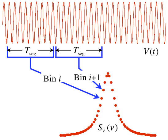
Figure 7: (Color online) Illustration of how a swept SA generates a spectrum from a voltage waveform.

The process by which an SA converts a time domain signal into a frequency domain spectrum, illustrated in Fig. 7, includes various time scales that must be incorporated into a model SA. For the ith frequency bin in the spectrum, the LO frequency of the mixer is fixed at $\nu_{\textrm{LO}}^{i}$ during a segment time $T_{\textrm{seg}}$ (although SAs often sweep the LO continuously, here we consider it to be stepped discretely). The mixer IF output goes through a bandpass filter, whose width is set by the resolution bandwidth (RBW) of the SA, and then through a power detector . The power detected during the ith segment is the value of $S_{V}$ for the ith frequency bin. For a spectrum spanning $n$ frequency bins, the time to acquire a single spectrum is $T_{\textrm{sweep}}=nT_{\textrm{seg}}$. When $N$ spectra are averaged together, the time to restabilize $\nu_{\textrm{LO}}$ at the first bin is typically much larger than $T_{\textrm{sweep}}$ and thus the total measurement time $T_{\textrm{meas}}$ is much larger than $NT_{\textrm{sweep}}$. Although this picture omits many details of the inner workings of an actual SA, it contains the relevant time scales that determine how non-white frequency noise affects the spectrum.

We created a model SA that takes $V_{\textrm{IF}}(t)$ as the input, rather than $V(t)$, since this is the data we recorded for our STOs. Thus rather than changing $\nu_{\textrm{LO}}$ to generate different frequency bins, we changed the center frequency of the bandpass filter. After filtering each segment (using a filter with 3 dB points at half the RBW away from the center frequency and a rolloff of $36\,\mathrm{dB/decade}$), we computed the “power” in each bin by simply summing the squares of the values in the segment . From each set of $n$ segments we obtained a single spectrum, and we repeated the process to obtain $N$ individual spectra for each value of $T_{\textrm{seg}}$. We fit the individual $S_{V}(\nu)$ to determine $\Delta\nu_{\textrm{SA}}$ for $T_{\textrm{meas}}=nT_{\textrm{seg}}$ and we fit the average $S_{V}(\nu)$ to determine $\Delta\nu_{\textrm{SA}}$ for $T_{\textrm{meas}}=NnT_{\textrm{seg}}$ (unlike in a real SA, there is no dead time between sweeps in our model SA). We used primarily the Voigt function to fit $S_{V}(\nu)$ because it can fit lines that are Lorentzian, Gaussian, or any mixture of the two. We first present the Voigt results and then discuss fits using pure Lorentzian and Gaussian functions.

Figure 8 shows Voigt linewidth vs. inverse measurement time for the Co/Ni device measured by (1) an actual SA, and (2) our model SA applied to the same $50\,\mathrm{ms}$ $V_{\textrm{IF}}(t)$ waveform used to compute $S_{\mathrm{\nu}}(f)$. For the model SA, we used $n=100$ and varied $T_{\textrm{meas}}$ by choosing values of $T_{\textrm{seg}}$ between $1\,\mathrm{\mu s}$ (shorter segments gave unreliable results) and $500\,\mathrm{\mu}s$. We report both the mean from fits to 10 individual spectra and the fit to the average of these 10 spectra. For the actual SA, we varied $T_{\textrm{meas}}$ by averaging with $N=1$, 2, 5, 10, 100, and 1000, repeating the measurement five times for each value of $T_{\textrm{meas}}$ in order to report a mean value and estimate its uncertainty. The actual and model SA results both show that $\Delta\nu_{\textrm{SA}}$ increases logarithmically with measurement time, and they agree quantitatively for $T_{\textrm{meas}}=1\,\mathrm{ms}$. When applied to the measured $V_{\textrm{IF}}(t)$ for the NiFe device, the model SA yields a weaker dependence of $\Delta\nu_{\textrm{SA}}$ on measurement time (the change in $\Delta\nu_{\textrm{SA}}$ barely exceeds the statistical uncertainty over the accessible range of $T_{\textrm{meas}}$), which is consistent with the weaker $1/f$ noise in $S_{\mathrm{\nu}}(f)$ for this device. We also applied the model SA to numerically generated signals. For signals having white frequency noise, $\Delta\nu_{\textrm{SA}}$ was independent of measurement time, whereas for signals having $S_{\mathrm{\nu}}(f)$ comparable to that measured for our Co/Ni device, $\Delta\nu_{\textrm{SA}}$ vs. $1/T_{\textrm{meas}}$ had a slope similar to that seen in Fig. 8. Thus the model SA applied to signals having a range of $S_{\mathrm{\nu}}(f)$ from strictly white to strongly $1/f$ indicates that the dependence of linewidth on measurement time is a direct consequence of non-white frequency noise.

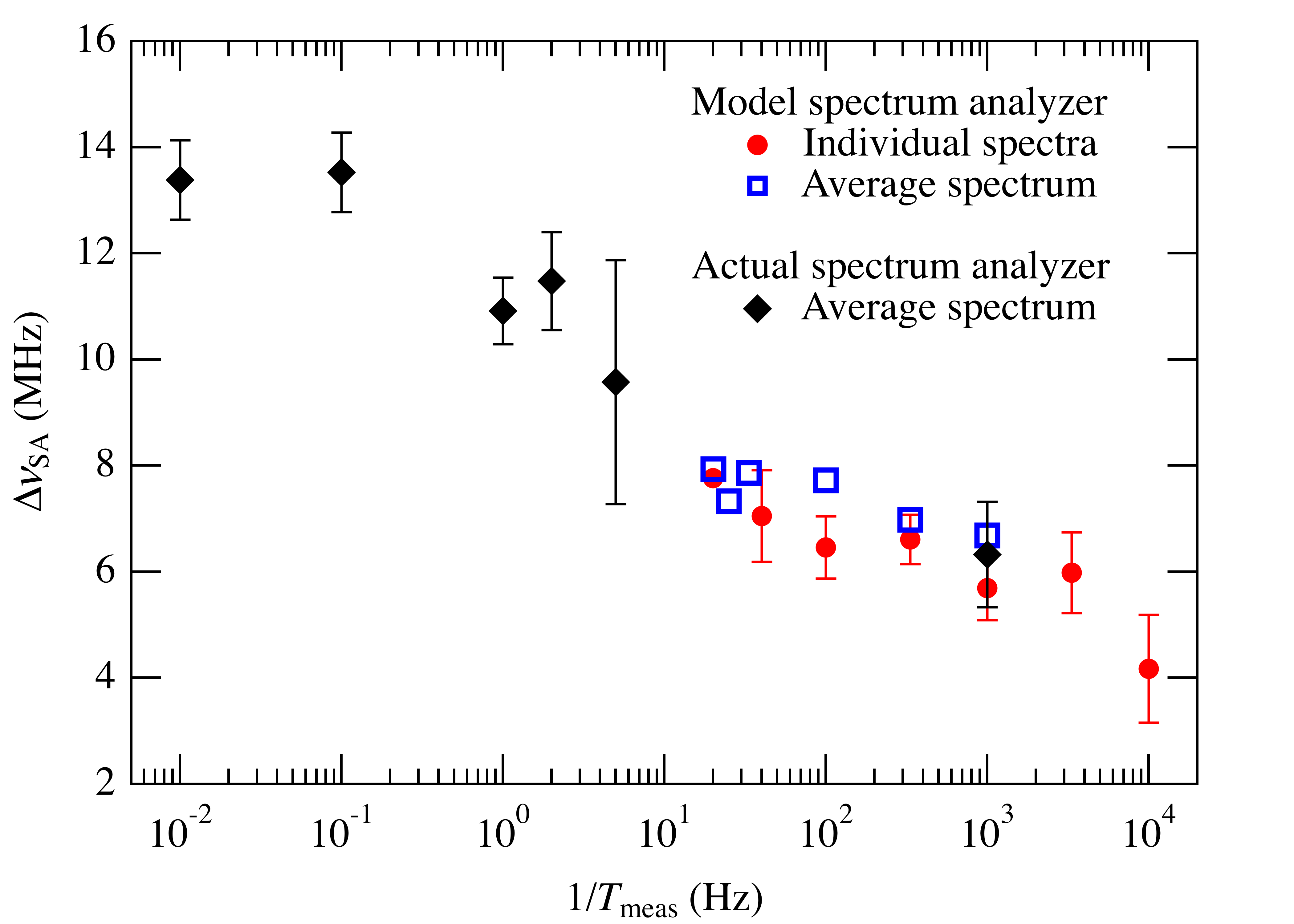
Figure 8: (Color online) Dependence of Voigt linewidth on inverse measurement time for the Co/Ni device. Model SA parameters are $\textrm{RBW}=1\,\mathrm{MHz}$, $n=100$, $N=10$ (except for the longest segments where the $50\,\mathrm{ms}$ IF waveform was used up before reaching 10 spectra). Error bars for solid circles show the standard deviation of the mean for a set of $N$ values with the same $T_{\textrm{meas}}$. Actual SA parameters are $\textrm{RBW}=1\,\mathrm{MHz}$, $T_{\textrm{sweep}}=1\,\mathrm{ms}$, dead time between sweeps $\approx 100\,\mathrm{ms}$. Error bars for solid diamonds show the standard deviation of the mean for a set of 5 successive measurements with the same $T_{\textrm{meas}}$.

As mentioned above, broadening due to $1/f$ frequency noise is accompanied by a change in the shape of the spectral line Mercer:1991zr ; Stephan:2005ly , with the Voigt shape changing from mostly Lorentzian to mostly Gaussian as $T_{\textrm{meas}}$ increases. The noise in our SA data for most values of $T_{\textrm{meas}}$ is too large to discern this trend clearly, i.e., a pure Lorentzian shape fits about as well as a Voigt shape. However, for the CoNi device at $T_{\textrm{meas}}\geq 10\,\mathrm{s}$ a Voigt shape clearly fits the data better than a Lorentzian shape, as shown in Fig. 9. We also show a pure Gaussian fit to this line for comparison, and we see that the Voigt function provides the best fit to the entire line. The Lorentzian shape gives a good fit to all spectra from the NiFe device, although we did not measure beyond $T_{\textrm{meas}}=1\,\mathrm{s}$ for the particular oscillation mode presented here. This is consistent with previous work on similar NiFe devices that did not find significant deviations from a Lorentzian line shape Rippard:2004ad ; Rippard:2004fr .

Figure 9: (Color online) Spectral line for Co/Ni device with $T_{\textrm{meas}}=10\,\mathrm{s}$. Lines show fits to Voigt, Gaussian, and Lorentzian functions.

In terms of the overall picture of STO spectral lines, our results mean there are two sources for a Gaussian contribution to line shape. The first involves the rate of relaxation to the stable precessional orbit, combined with the dependence of frequency on precessional amplitude (the “frequency nonlinearity” intrinsic to STOs Tiberkevich:2008ys ), which sets a correlation time for phase fluctuations. When this correlation time is short compared to the thermal dephasing time the line shape is Lorentzian; in the opposite limit it is Gaussian Tiberkevich:2008ys . In terms of frequency noise, this correlation suppresses $S_{\mathrm{\nu}}(f)$ at large $f$ according to

$$S_{\nu}(f)=\frac{S_{\textrm{wh}}}{1+(\nicefrac{{2\pi f}}{{\eta}})^{2}},$$ (5)

where $\eta$ is the relaxation rate SilvaKeller_preprint2010 . The second source for a Gaussian line shape is $1/f$ frequency noise, as described above, which can be understood as a correlation at long times that affects $S_{\mathrm{\nu}}(f)$ at small $f$.

Distinguishing the two mechanisms for a non-Lorentzian STO line shape clearly requires more than a single SA measurement. Since the relaxation mechanism does not depend on measurement time, SA measurements over a wide range of $T_{\textrm{meas}}$ could indicate whether the $1/f$ mechanism is significant, but a quantitative conclusion about the relative contributions of the two mechanisms would require considerable care. Another approach is to use the autocorrelation function of the STO signal to measure the correlation at short times, as done in recent experimental work Boone:2009fk where the deviation from a Lorentzian line shape was less pronounced than that seen in Fig. 9. Finally, both the relaxation rate and $1/f$ noise can be seen directly in $S_{\mathrm{\nu}}(f)$ if it is measured over a large enough range of $f$. This approach has the advantage that each mechanism can be quantified separately.

As mentioned above, in our measurements the limited IF bandwidth suppressed $S_{\mathrm{\nu}}(f)$ above $f\approx 20\,\mathrm{MHz}$. While this prevents a direct measurement of $\eta$, it does set a lower bound of $\eta/2\pi\approx 20\,\mathrm{MHz}$ (see Eq. (5)). From the theory of the relaxation mechanism Tiberkevich:2008ys ; SilvaKeller_preprint2010 , the condition for a negligible Gaussian contribution can be written as $\eta/2\pi\gg\Delta\nu_{\textrm{wh}}$. Since the measured values of $\Delta\nu_{\textrm{wh}}$ ($10.4\,\mathrm{MHz}$ for the NiFe device; $4.1\,\mathrm{MHz}$ for the Co/Ni device) are less than $20\,\mathrm{MHz}$, we can conclude that the line shape for both devices would be close to Lorentzian in the absence of $1/f$ noise. The strongly non-Lorentzian line in Fig. 9 for the Co/Ni device can be unambiguously attributed to $1/f$ frequency noise.

Although non-white frequency noise has not been directly measured in previous STO experiments, recent reports indicate it is probably an important effect in devices beyond the two types considered here. The line “jitter” and SA linewidth increasing with measurement time reported in MgO nanopillar STOs Devolder:2009ve can both be interpreted as evidence for $1/f$ frequency noise, and the authors suggest a possible mechanism for such noise that is specific to their particular devices. In other nanopillar STOs containing MgO Houssameddine:2009zm or metallic Pribiag:2009by barriers, the DFT of selected short segments yielded linewidths much smaller than those found from either DFT or SA measurements averaged over long times. Beyond these published reports, we and others have noticed when watching the non-averaged SA display that some devices show larger trace-to-trace jumps in center frequency than others, an observation that may be explained by varying amounts of $1/f$ noise in the devices.

VI Conclusion

We measured the output of two types of STOs in the time domain, using the IF ouput of an SA to access signals well above 10 GHz. We presented two techniques for obtaining the power spectrum of frequency noise, $S_{\mathrm{\nu}}(f)$, and showed the advantage of combining them to yield an averaged $S_{\mathrm{\nu}}(f)$ over a wide range of $f$. The $1/f$ noise we observed indicates that theoretical models based on thermal noise sources are insufficient for our devices over times longer than about $1\,\mathrm{\mu s}$. We also measured spectral linewidths in our devices using both an actual SA and a numerical model that allowed shorter measurement times. For the devices with the strongest $1/f$ noise, we found that SA linewidth increased, and the line shape became significantly non-Lorentzian, as measurement time increased. These results imply that SA measurements of STOs should be accompanied by measurement time values so that (1) comparisons can be made among various STOs measured by different researchers, and (2) non-Lorentzian line shapes can be correctly interpreted. Although the consequences of our results for STO applications depend on the time scales involved, we expect that measurements of $S_{\mathrm{\nu}}(f)$ will allow more accurate predictions of performance than SA measurements alone for many applications. The detailed picture of oscillator noise provided by $S_{\mathrm{\nu}}(f)$ will also help in distinguishing among different physical origins for the noise.

References

- (1) D. C. Ralph and M. D. Stiles, “Spin transfer torques,” J. Magn. Magn. Mater., vol. 320, no. 7, pp. 1190–1216, 2008.
- (2) T. J. Silva and W. H. Rippard, “Developments in nano-oscillators based upon spin-transfer point-contact devices,” J. Magn. Magn. Mater., vol. 320, pp. 1260–1271, 2008.
- (3) J. A. Katine and E. E. Fullerton, “Device implications of spin-transfer torques,” J. Magn. Magn. Mater., vol. 320, pp. 1217–1226, 2008.
- (4) V. Tiberkevich, A. Slavin, and J.-V. Kim, “Microwave power generated by a spin-torque oscillator in the presence of noise,” Appl. Phys. Lett., vol. 91, p. 192506, 2007.
- (5) J.-V. Kim, V. Tiberkevich, and A. N. Slavin, “Generation linewidth of an auto-oscillator with a nonlinear frequency shift: Spin-torque nano-oscillator,” Phys. Rev. Lett., vol. 100, p. 017207, 2008.
- (6) J.-V. Kim, Q. Mistral, C. Chappert, V. S. Tiberkevich, and A. N. Slavin, “Line shape distortion in a nonlinear auto-oscillator near generation threshold: Application to spin-torque nano-oscillators,” Phys. Rev. Lett., vol. 100, p. 167201, 2008.
- (7) V. S. Tiberkevich, A. N. Slavin, and J.-V. Kim, “Temperature dependence of nonlinear auto-oscillator linewidths: Application to spin-torque nano-oscillators,” Phys. Rev. B, vol. 78, p. 092401, 2008.
- (8) K. Kudo, T. Nagasawa, R. Sato, and K. Mizushima, “Amplitude-phase coupling in a spin-torque nano-oscillator,” J. Appl. Phys., vol. 105, p. 07D105, 2009.
- (9) T. J. Silva and M. W. Keller, “Theory of thermally induced phase noise in spin torque oscillators for a high-symmetry case.” To appear in IEEE Trans. Magn., 2010.
- (10) P. Lesage and C. Audoin, “Characterization and measurement of time and frequency stability,” Radio Science, vol. 14, pp. 521–539, 1979.
- (11) M. Lax, “Classical noise V. Noise in self-sustained oscillators,” Phys. Rev., vol. 160, pp. 290–307, 1967.
- (12) G. H. O. Daalderop, P. J. Kelly, and F. J. A. den Broeder, “Prediction and confirmation of perpendicular magnetic anisotropy in Co/Ni multilayers,” Phys. Rev. Lett., vol. 68, pp. 682–685, 1992.
- (13) M. R. Pufall, W. H. Rippard, M. L. Schneider, and S. E. Russek, “Low-field current-hysteretic oscillations in spin-transfer nanocontacts,” Phys. Rev. B, vol. 75, p. 140404, 2007.
- (14) W. H. Rippard, A. M. Deac, M. R. Pufall, J. M. Shaw, M. W. Keller, S. E. Russek, G. E. W. Bauer, and C. Serpico, “Spin-transfer dynamics in spin valves with out-of-plane magnetized CoNi free layers,” Phys. Rev. B, vol. 81, p. 014426, 2010.
- (15) W. H. Press, S. A. Teukolsky, W. T. Vetterling, and B. P. Flannery, Numerical Recipes: The Art of Scientific Computing. Cambridge Univ. Press, 3 ed., 2007.
- (16) M. W. Keller, A. B. Kos, T. J. Silva, W. H. Rippard, and M. R. Pufall, “Time domain measurement of phase noise in a spin torque oscillator,” Appl. Phys. Lett., vol. 94, p. 193105, 2009.
- (17) C. Henry, “Theory of the linewidth of semiconductor lasers,” Quantum Electronics, IEEE Journal of, vol. 18, pp. 259 – 264, 1982.
- (18) L. Mercer, “1/f frequency noise effects on self-heterodyne linewidth measurements,” J. Lightwave Technol., vol. 9, pp. 485 –493, 1991.
- (19) G. M. Stéphan, T. T. Tam, S. Blin, P. Besnard, and M. Têtu, “Laser line shape and spectral density of frequency noise,” Phys. Rev. A, vol. 71, p. 043809, 2005.
- (20) T. Okoshi, K. Kikuchi, and A. Nakayama, “Novel method for high resolution measurement of laser output spectrum,” Electron. Lett., vol. 16, pp. 630–631, 1980.
- (21) W. H. Rippard, M. R. Pufall, S. Kaka, T. J. Silva, and S. E. Russek, “Current-driven microwave dynamics in magnetic point contacts as a function of applied field angle,” Phys. Rev. B, vol. 70, p. 100406, 2004.
- (22) W. H. Rippard, M. R. Pufall, S. Kaka, S. E. Russek, and T. J. Silva, “Direct-current induced dynamics in Co90Fe10/Ni80Fe20 point contacts,” Phys. Rev. Lett., vol. 92, p. 027201, 2004.
- (23) C. Boone, J. A. Katine, J. R. Childress, J. Zhu, X. Cheng, and I. N. Krivorotov, “Experimental test of an analytical theory of spin-torque-oscillator dynamics,” Phys. Rev. B, vol. 79, p. 140404, 2009.
- (24) T. Devolder, L. Bianchini, J.-V. Kim, P. Crozat, C. Chappert, S. Cornelissen, M. O. de Beeck, and L. Lagae, “Auto-oscillation and narrow spectral lines in spin-torque oscillators based on MgO magnetic tunnel junctions,” J. Appl. Phys., vol. 106, p. 103921, 2009.
- (25) D. Houssameddine, U. Ebels, B. Dieny, K. Garello, J.-P. Michel, B. Delaet, B. Viala, M.-C. Cyrille, J. A. Katine, and D. Mauri, “Temporal coherence of MgO based magnetic tunnel junction spin torque oscillators,” Phys. Rev. Lett., vol. 102, no. 25, p. 257202, 2009.
- (26) V. S. Pribiag, G. Finocchio, B. J. Williams, D. C. Ralph, and R. A. Buhrman, “Long-timescale fluctuations in zero-field magnetic vortex oscillations driven by dc spin-polarized current,” Phys. Rev. B, vol. 80, p. 180411, 2009.