Interface mapping in two-dimensional random lattice models

Abstract

We consider two disordered lattice models on the square lattice: on the medial lattice the random field Ising model at $T=0$ and on the direct lattice the random bond Potts model in the large-$q$ limit at its transition point. The interface properties of the two models are known to be related by a mapping which is valid in the continuum approximation. Here we consider finite random samples with the same form of disorder for both models and calculate the respective equilibrium states exactly by combinatorial optimization algorithms. We study the evolution of the interfaces with the strength of disorder and analyse and compare the interfaces of the two models in finite lattices.

I Introduction

The presence of different type of quenched disorder could influence the cooperative behaviour of many-body systems in different measure. In this respect dilution or random ferromagnetic bonds, which are often called as $T_{c}$-disorder, have a relatively weak effect. The ferromagnetic order in the pure system, which is present for $T<T_{c}$, is not destroyed by a small amount of $T_{c}$-disorder. Dilution has a dramatic effect only in the vicinity of a phase transition point, $|T-T_{c}|/T_{c}\ll 1$. If this transition is of second order even its universality class can be changed for any small amount of disorderharris .

A disorder perturbation with a stronger effect is represented by random fieldsnatt . As an example we consider here the random field Ising model (RFIM) in which the fields are taken from a distribution with zero mean and variance $h_{0}^{2}$. In dimensions, $d>2$, the phase transition is governed by a zero-temperature fixed point, the ground state of the system being disordered for $h_{0}>h_{0,c}(d)>0$, and there is magnetic long-range-order for $h_{0}<h_{0,c}(d)$. In two-dimensions we have $h_{0,c}(2)=0$, thus the magnetic order in the ground state is destroyed by any finite random fieldimryma ; aizenmanwehr . The ground state of the RFIM is conveniently characterized by geometric (or Ising) clustersdroplet , which are formed by adjacent spins being in the same orientation. In $2d$ these clusters are homogeneous only up to a finite characteristic length, $\ell_{g}$, which is called the breaking-up length of geometrical clusterslb ; seppala ; kornyei . In a coarse-grained picture the ground state consists of randomly oriented domains of typical size, $\ell_{g}$, and as a consequence there is no long-range-order in the system. For weak disorder, $h_{0}\ll J$, $J=1$ being the nearest neighbour coupling constant, the breaking-up length is large, and for $h_{0}\to 0$ it diverges aslb :

$$\ell_{g}(h_{0})\sim\exp(Ah_{0}^{-2})\;,$$ (1)

with a disorder dependent constant, $A=O(1)$.

As far as first-order transitions are concerned the effect of bond disorder is also strong and the physical phenomena is analogous to that of the RFIM discussed beforeCardy99 . As a prototypical model having a first-order phase transition we consider the $q$-state Potts modelWu in which the number of states is sufficiently large, $q>q_{c}(d)$. In the pure system having homogeneous couplings ($J=J_{0}$) at the first-order transition point, $T=T_{c}$, the ordered and disordered phases coexist, the latent heat is finite and there is a finite jump of the order-parameter. Introducing random ferromagnetic couplings, such that the fluctuating part, $\kappa=\dfrac{J-J_{0}}{J_{0}}$, has zero mean and variance $\kappa_{0}^{2}$ the latent heat and the jump of the magnetization is generally reduced with increasing $\kappa_{0}$. In dimensions $d>2$ for weak disorder, $\kappa_{0,c}(d)>\kappa_{0}>0$, the transition stays first order, whereas for strong disorder, $\kappa_{0}>\kappa_{0,c}(d)$, the latent heat is vanishing and the transition softens to second orderimrywortis ; aizenmanwehr . The critical exponents of this transition are independent of the strength of disorder, but they generally depend on the value of $q$pottsmc ; pottstm ; olson99 ; ai03 ; long2d . In the borderline case, $\kappa_{0}=\kappa_{0,c}(d)$, there is a tricritical point with a new class of tricritical exponents, which are expected to be independent of the value of $q$ and the actual fixed point is at $q\to\infty$mai05 . In $2d$ the limiting value is $\kappa_{0,c}(2)=0$ and the phase transition is softened to second order by any weak bond disorderimrywortis ; aizenmanwehr .

To characterize the state of the system we consider the high-temperature series expansionkasteleyn , which in the large-$q$ limit is dominated by a single diagram. In the pure case this diagram is either the fully connected graph, which happens in the ordered phase, $T<T_{c}$, or the fully disconnected graph, which is the case in the disordered phase, $T>T_{c}$. At the phase transition point these two basic graphs coexist. In the disordered model the dominant diagram at $T=T_{c}$ contains both connected and disconnected parts. In $2d$ the optimal diagram is homogeneous only up to a characteristic finite length, $\ell_{d}$, which is the breaking-up length of the optimal diagram. For small disorder the breaking-up length is large and in the limit $\kappa_{0}\to 0$ it is divergentmai05 :

$$\ell_{d}(\kappa_{0})\sim\exp(B\kappa_{0}^{-2})\;,$$ (2)

which is in the same form, as for the RFIM in Eq.(1). In the thermodynamic limit the optimal diagram is a random composition of the two basic graphs of typical size, $\ell_{d}$, therefore there is no phase coexistence in $2d$ and the transition is of second order.

As described above the RFIM and the random bond Potts model (RBPM) have analogous physical properties. This analogy was first noticed by Cardy and Jacobsen pottstm (CJ) and they have obtained an exact mapping, which is valid in the limit of $d\to 2$ and $q\to\infty$, when the interface Hamiltonian of the two problems have the same type of solid-on-solid (SOS) description. From this mapping follows that the energy exponents of the tricritical RBPM are equivalent to the magnetization exponents of the critical RFIM. Furthermore, analyzing the renormalization group (RG) flow it was conjectured that the above mapping stays valid for $d>2$, in particular at $d=3$. This conjecture has been numerically tested mai05 for the $3d$ RBPM in the large-$q$ limit.

The CJ-mapping has consequences at $d=2$, as far as interface properties of the two models are concerned at large scales. This has already been mentioned with respect to the same form of the breaking-up lengths in Eqs.(1) and (2). In this context one may ask the question how this mapping works in finite scales? In this paper we are going to perform a systematic study and consider both models with exactly the same form of disorder. For this we put the Potts model on the square lattice, whereas the Ising model on the medial lattice. In this way couplings of the Potts model and fields of the Ising model are on the same position. We study random samples with fixed boundary conditions, which prefer the opposite orientation for the RFIM and the different phases (basic graphs) for the RBPM at the two halves of the lattice. Using combinatorial optimization algorithmheiko ; aips02 we calculate exactly the ground state of the RFIM and the optimal diagram of the RBPM and study their evolution with increasing the strength of disorder. We also compare the diagrams obtained in the two problems and study their fitting.

The structure of the rest of the paper is the following. The RFIM and the RBPM are defined in Sec.II together with the asymptotic mapping. Evolution of the diagrams with the strength of disorder are presented in Sec.III whereas a comparison of the diagrams of the two models are shown in Sec.IV. Our paper is closed by a discussion in Sec.V.

II Models and asymptotic mapping

We consider a square lattice the sites of which are at $(x,y)$ with $1\leq x\leq L$ and $-(L-1)/2\leq y\leq(L-1)/2$ and both $x$ and $y$ being integer. In the corresponding medial lattice the sites are placed to the middle of the links and have coordinates $(u,v)$ as $(x,y+1/2)$ and $(x+1/2,y)$, see Fig.1.

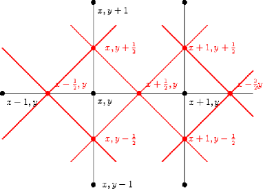
Figure 1: The square lattice (black) with the Potts spins and its medial lattice (red) with the Ising spins.

II.1 Random field Ising model

Spins of the random field Ising model, $\sigma_{u,v}=\pm 1$, are put on the vertices of the medial lattice. The Hamiltonian of the model is given by:

$${\cal H_{I}}=-\sum_{u,v}\sigma_{u,v}\sigma_{u+1/2,v\pm 1/2}-\sum_{u,v}h(u,v)\sigma_{u,v}\;.$$ (3)

The external field, $h(u,v)$, is a random number which is parametrized as:

$$h(u,v)=h_{0}\epsilon(u,v)\;,$$ (4)

where the distribution of $\epsilon(u,v)$ has zero mean and variance unity. We apply fixed spin boundary conditions: the Ising spins at the upper part of the boundary ($v>0$) are fixed to $+1$, and at the lower part of the boundary ($v<0$) they are fixed to $-1$. This model is studied at $T=0$. For a given realization of the disorder we calculate the ground state exactly by a combinatorial optimization algorithm.

II.1.1 SOS approximation

For weak disorder, such that $\ell_{g}(h_{0})>L$, the ground state is well approximated by two clusters with $+1$ and $-1$ spins, respectively, and having an interface in between. Furthermore we use the solid-on solid (SOS) approximation, when the height of the interface at position $u$ is given by a unique function, $\zeta(u)$. In this case the position of the interface is obtained by minimizing the SOS energy functionalpottstm :

$$E(\zeta)=-h_{0}\sum_{{u}}\left(\sum_{v<\zeta(u)}-\sum_{v>\zeta(u)}\right)\epsilon(u,v)\;,$$ (5)

with the constrain that the length of the interface, measured in the medial lattice is constant.

II.2 Random bond Potts model

The random bond Potts model is put on the vertices of the original square lattice and defined by the Hamiltonian:

$${\cal H_{P}}=-\sum_{x,y} [ J(x,y+1/2)\delta(s_{x,y},s_{x,y+1})$$

$$+ J(x+1/2,y)\delta(s_{x,y},s_{x+1,y})]\;.$$

Here $s_{x,y}=1,2,\dots,q$ is a Potts spin variable at site $(x,y)$ and the couplings, $J(x,y+1/2)\equiv J(u,v)>0$ and $J(x+1/2,y)\equiv J(u,v)>0$, are independent and identically distributed random numbers. Introducing the reduced temperature, $T^{\prime}=T\ln q$, and similarly, $\beta^{\prime}=1/T^{\prime}=\beta/\ln q$, the partition function in the random cluster representation is given bykasteleyn :

$$Z=\sum_{G\subseteq E}q^{c(G)}\prod_{(u,v)\in G}\left[q^{K(u,v)}-1\right]$$ (7)

with $K(u,v)=\beta^{\prime}J(u,v)$. Here the sum runs over all subset of bonds, $G\subseteq E$ and $c(G)$ stands for the number of connected components of $G$. In the following we consider the large-$q$ limit, where $q^{K(u,v)}\gg 1$, and the partition function can be written as

$$Z=\sum_{G\subseteq E}q^{\phi(G)},\quad\phi(G)=c(G)+\sum_{(u,v)\in G}K(u,v)$$ (8)

which is dominated by the largest term, $\phi^{*}=\max_{G}\phi(G)$, so thatJRI01 ; ai03

$$Z=q^{\phi^{*}}+{\rm subleading~{}terms}.$$ (9)

For random couplings with $0<K(u,v)<1$ we use the form, $K(u,v)=K(1+\kappa(u,v))$ and the $\kappa(u,v)$ random numbers are taken from a symmetric distribution: $P(\kappa)=P(-\kappa)$, with a variance $\kappa_{0}^{2}$, thus $\kappa(u,v)=\kappa_{0}\epsilon(u,v)$. For this type of distribution the phase transition point of the system follows from self-duality and given bydom_kinz :

$$K_{c}=\frac{1}{2}.$$ (10)

Thus at the critical point the random couplings are parametrized as:

$$\beta^{\prime}J(u,v)=K(u,v)=\dfrac{1}{2}\left[1+\kappa_{0}\epsilon(u,v)\right]\;$$ (11)

and the strength of disorder is measured by $\kappa_{0}$. In our problem we use such type of boundary conditions, that the boundary couplings at the upper part of the lattice $(v>0)$ are strong $\kappa^{+}=1$, thus promoting an ordered phase, whereas at the lower part of the lattice $(v<0)$ these are weak, $\kappa^{-}=0$, thus favouring the disordered phase. For a given realization of the disorder we calculate the ground state exactly by a combinatorial optimization algorithmaips02 .

II.2.1 SOS approximation

In the following we consider the model at the critical point in the weak disorder limit, when $\ell_{d}(\kappa_{0})>L$. In this case we use the approximation that the optimal diagram consists of a fully connected part, denoted by $G_{c}$, and a fully disconnected part, denoted by $\overline{G_{c}}$, having an interface in between. The interface is approximated with the solid-on-solid (SOS) model: having a unique height $\zeta(u)$ at position $u$pottstm ; long2d . The lattice contains $N=L^{2}$ points, from which $n(G_{c})$ and $n(\overline{G_{c}})$ are in $G_{c}$ and in $\overline{G_{c}}$, respectively. Similarly, out of the $E=2L(L-1)$ edges, there are $e(G_{c})$ in the subgraph, $G_{c}$. The cost function in Eq.(8) is given by:

$$\phi = N+1-n(G_{c})+\sum_{(u,v)\in G}(1+\kappa_{0}\epsilon(u,v))/2$$

$$= N+1-n(G_{c})-e(G_{c})/2+\sum_{(u,v)\in G}\kappa_{0}\epsilon(u,v)/2\;.$$

Now we use the microcanonical condition: $\sum_{all~{}bonds}\epsilon(u,v)=0$ and arrive to the cost function:

$$4\phi(\zeta)=\kappa_{0}\sum_{{u}}\left(\sum_{v<\zeta(u)}-\sum_{v>\zeta(u)}\right)\epsilon(u,v)\;,$$ (13)

for a fixed value of $n(G_{c})-e(G_{c})/2$. This latter quantity is uniquely determined by the length of the interface, which is measured in the square lattice.

Comparing the two expressions in Eqs.(5) and (13) we see that in the SOS approximation the position of the interface is obtained by finding the extremal value of the same expression, however with somewhat different constrains. In both cases the length of the interface is fixed, however in the RFIM this length is measured in the medial lattice, whereas for the RBPM in the original lattice. In the following we study both models numerically and see how well the SOS approximation and thus the above relation is valid in finite systems.

III Evolution of interfaces with the strength of disorder

In the numerical study we use bimodal disorder, such that $\epsilon(u,v)=\pm 1$ with the same probability.

III.1 Random field Ising model

For RFIM the evolution of the ground state with the strength of disorder, $h_{0}$, for a given realization of the random numbers, $\epsilon(u,v)$, is illustrated in Fig.2. In the limit $h_{0}\to 0^{+}$ there is a unique SOS interface between two oppositely magnetized clusters. With increasing $h_{0}$ at $h_{0,1}$ the ground state will change. It still consists of two large clusters, however the interface have some overhangs, thus it is no-longer of SOS type. With further increased disorder, for $h_{0}\geq h_{0,2}$, no longer two clusters exist, but some islands are formed in the big clusters. Finally, for strong disorder, $h>h_{0,3}$, the ground state is represented by several disjoint clusters and one can not identify an interface in the systempercolation .

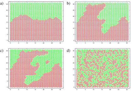
Figure 2: Evolution of the ground state of the RFIM with increasing strength of disorder in a $32\times 32$ lattice. Up and down spins are represented by dark (red) and light (green) regions. a) $h_{0}=0.1275$: Two clusters with an SOS interface. b) $h_{0}=0.2525$: Two clusters with an interface with overhangs. c) $h_{0}=0.3275$: Internal islands are formed within the big clusters. d) $h_{0}=4.0$: Several disjoint clusters are formed.

We have studied the behavior of the first relevant disorder scale, $h_{0,1}$, at which the SOS picture is broken down. Having several samples we have calculated its mean value, which is then repeated for different finite sizes, $L$. $\overline{h}_{0,1}(L)$ is found to go to zero with $L$ as a power-low, $\overline{h}_{0,1}(L)\sim L^{-\omega}$, which is illustrated in Fig.3. The exponent is found to be: $\omega=0.36(5)$. Similarly, the second disorder scale, $h_{0,2}$, is found to follow the same type of decay with $L$, with the same exponent, $\omega$, but with a different prefactor.

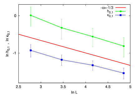
Figure 3: Average value of the critical disorder strength for the RFIM, $h_{0,1}$, and that for the RBPM, $\kappa_{0,1}$, as a function of $L$ in log-log scale. The straight line indicating the theoretical prediction has a slope $-\omega=-1/3$.

Our numerical results are in agreement with the exact result, that for any finite $h_{0}>0$ in the thermodynamic limit there is no long range order in the $2d$ RFIM.

III.2 Random bond Potts model

We have repeated the previous analysis for the RBPM. For a given random sample we have varied the strength of disorder, $\kappa_{0}$, and studied the form of the optimal diagram. Having the same set of $\epsilon(u,v)$ as for the RFIM in Fig.2 the results are collected in Fig.4. In the limit $\kappa_{0}\to 0$ the interface is plane, with a minimal length, $L_{int}=L$ (not shown in Fig.4). At a limiting value, $\kappa_{0,0}$, the interface becomes an SOS interface with $L_{int}>L$. Further increasing $\kappa_{0}$ the length of the interface is increasing, but it stays SOS type. Afterwards, at $\kappa_{0,1}$ the interface will loose its SOS character: overhangs and bubbles appear. Finally, for strong disorder the optimal diagram is composed of disjoint subgraphs. We can thus conclude that the evolution of the interfaces in the RBPM and in the RFIM with the strength of disorder are qualitatively very similar. There are, however, differences, for $\kappa_{0}\leq\kappa_{0},0$, which are due to the different orientations of the interface lines.

We have also studied the size dependence of the average value of $\kappa_{0,1}$, which is shown in Fig.3. Here also a power-low decay is found with the same exponent, $\omega$, as for the RFIM.

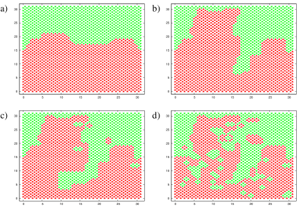
Figure 4: Evolution of the optimal set of the RBPM with increasing strength of disorder in a $32\times 32$ lattice having the same set of $\epsilon(u,v)$ as for the RFIM in Fig.2. Connected graphs and isolated sites are represented by dark (red) and light (green) regions. a) $\kappa_{0}=0.25$: Two clusters with an SOS interface. b) $\kappa_{0}=0.34$: Two clusters with an interface with overhangs. c) $\kappa_{0}=0.5$: Internal islands are formed within the big clusters. d) $\kappa_{0}=0.76$: Several disjoint clusters are formed.

We can explain the value of the $\omega$ exponent, which is measured both for the RFIM and for the RBPM, in the following way. Let us concentrate now on the RFIM, for the RBPM similar reasoning works. At $h_{0,1}$ the first overhang in the ground state of the RFIM appears. The difference between the ground states for $h<h_{0,1}$ and $h>h_{0,1}$ has a narrow shape. Its typical width is $w=O(1)$, since the total length of the interface is increased by $\Delta L_{int}=O(1)$, and its height is given by $L_{\perp}$, which is the size of the transverse fluctuations of the SOS interface and given byGwa_Spohn : $L_{\perp}\sim L^{2/3}$. Now we use the Imry-Ma argumentimryma and compare the loss of energy due to the increase of the interface: $E_{int}\sim w$, with that of the gain due to disorder fluctuations: $E_{fl}\sim h_{0,1}\sqrt{wL_{\perp}}$. From the condition: $E_{int}=E_{fl}$ we obtain the estimate $h_{0,1}\sim L^{-1/3}$, thus the exponent is given by $\omega=1/3$ in agreement with the numerical results.

IV Comparison of the structure of the graphs in the two models

The SOS mappings presented in Sec.II assure that for weak disorder the scaling behavior of the interfaces in the two models are asymptotically equivalent. Here we study the question what happens for finite systems and for not too weak disorder, which type of similarity occurs between the ground states of the two problems. For this study we consider exactly the same random samples for the two models, which means that the set of random variables, $\epsilon(u,v)$, are the same for each position, $(u,v)$, just the strength of disorder, $h_{0}$ and $\kappa_{0}$, respectively, can be different. For a given sample we calculate the ground state of the RFIM, as well as the optimal set of the RBPM and compare them. In order to define a quantitative measure of the difference between the two graphs we consider the medial lattice and assign to each site, $(u,v)$, a variable denoted by $D(u,v)$. If in the ground state of the RFIM $\sigma(u,v)=+1$ ($\sigma(u,v)=-1$) and at the same time in the optimal set of the RBPM the edge $(u,v)$ is occupied (non-occupied), then $D(u,v)=0$, otherwise $D(u,v)=1$. In Fig.5 we compare the ground state configurations in Fig.2 with the optimal sets in Fig.4. One can see in this figure that close to the boundaries $D(u,v)$ is typically zero (Greyscale (gsc) 3 (red) and gsc 2 (green) points) and in the interface region we have sites with $D(u,v)=1$ (gsc 4 (blue) and gsc 1 (yellow) points). The difference between the two graphs is defined by the fraction of non-coherent sites:

$$\delta(h_{0},\kappa_{0})=\dfrac{1}{2L(L-1)}\sum_{(u,v)}D(u,v)\;,$$ (14)

what we call as discrepancy. Here $2L(L-1)$ is the number of sites in the medial lattice with the given boundary condition.

In the actual calculation we have fixed the value of the RBPM disorder parameter, $\kappa_{0}$, and calculated the discrepancy for different values of $h_{0}$. In this way we have measured the minimum value of the discrepancy, $\delta_{min}(\kappa_{0})$, and the corresponding value of the RFIM parameterh0min , $\tilde{h}_{0}$. The average value of the minimal discrepancy, $[\delta_{min}]_{\rm av}(\kappa_{0})$ versus $\kappa_{0}$ is plotted in Fig.6 for different finite systems from $L=16$ to $L=128$.

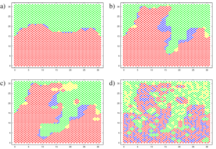
Figure 5: Comparison of the ground state of the RFIM with the optimal set of the RBPM for the same pair of disorder parameters ($h_{0}$ and $\kappa_{0}$) as given in the panels of Figs.2 and 4, respectively. Greyscale (gsc) 3 (red) points represent: up spins in the RFIM and the connected graph in the RBPM; gsc 2 (green) points: down spins and isolated sites; gsc 4 (blue) points: down spins and connected graph; gsc 1 (yellow) points: up spins and isolated sites. The gsc 4 (blue) and gsc 1 (yellow) points are non-coherent sites. The values of the discrepancies are $\delta=24/1984$, $135/1984$, $187/1984$ and $559/1984$, for panels $a)$, $b)$, $c)$ and $d)$, respectively.

For large $\kappa_{0}$ the curves have a plateau, then with decreasing $\kappa_{0}$ they start to decrease, pass over a minimum and afterwards increase for small $\kappa_{0}$. With increasing size the value at the minimum $[\delta_{min}]_{\rm av}^{min}(L)$ is decreasing and in the large-$L$ limit the minimum is expected to be shifted at the origin. Indeed in the inset of Fig.6 we have plotted $[\delta_{min}]_{\rm av}^{min}(L)$ as a function of $L$ and in a log-log scale an asymptotically linear dependence is found, thus $[\delta_{min}]_{\rm av}^{min}(L)\sim L^{-\omega^{\prime}}$. Here the exponent is $\omega^{\prime}=0.39(7)$, which is compatible with $\omega^{\prime}=1/3$, the value of which follows from the following simple argument. For weak disorder the interface in the RBPM is approximately flat (see the reasoning in Sec.III) whereas in the RFIM it is rough having a transverse fluctuation of size $L_{\perp}\sim L^{2/3}$. In the interface region there are $L\times L_{\perp}$ sites, consequently the average discrepancy behaves as $\sim L^{-1/3}$, in agreement with the numerical results. We can thus conclude that in the large-$L$ limit the behavior of the discrepancy with the strength of disorder is the following. It starts from zero at $\kappa_{0}=0$, has an approximately quadratic variation for small disorder and approaches a plateau for stronger disorder. This behavior is in complete agreement with the SOS mapping in Sec.II).

We have also checked the actual form of the graphs in the two problems for strong disorder. As illustrated in Fig.5 the two graphs generally have quite similar structure, as far as the subgraphs, the topology of the islands, etc. are concerned.

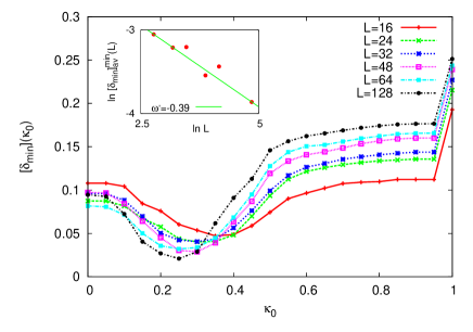
Figure 6: Average value of the minimal discrepancy as a function of the disorder parameter $\kappa_{0}$ for different finite systems. In the inset the minimal value of $[\delta_{min}]_{\rm av}(\kappa_{0})$ is plotted as a function of $L$ in a log-log scale. Here the straight line has a slope of $\omega^{\prime}=0.39$, to be compared with the theoretical prediction: $1/3$.

V Discussion

In this paper we have considered two problems of lattice statistics in which disorder has a strong and somewhat analogous effect as far as the cooperative behavior of the models are considered. In both problems geometrical interpretation of the state of the system is used. In the first problem, which is the two-dimensional Ising model we use clusters of parallel spins (geometrical clusters) to characterize the ground state. Here random fields destroy the ferromagnetic order at $T=0$ and the geometrical clusters have homogeneous parts of finite extent, $\ell_{g}(h_{0})$. In the second problem, which is the two-dimensional Potts model with a large number of states the optimal diagram of the high-temperature series expansion is used as a geometrical interpretation. Here we consider the first-order transition point of the pure system, which transition is softened to a continuous one due to bond disorder. As a consequence at the transition point there is no phase-coexistence and the homogeneous parts of the optimal diagram have a finite extent of $\ell_{d}(\kappa_{0})$.

In this paper we have considered finite samples of linear length, $L$, by varying the strength of disorder, $h_{0}$ and $\kappa_{0}$ in the two problems, respectively. Having fixed spin boundary conditions for $\ell_{g}(h_{0})>L$ ($\ell_{d}(\kappa_{0})>L$) there are basically two phases (two elementary diagrams) in the ground state (optimal diagram) of the RFIM (RBPM), which are separated by an interface. For large scales and in the SOS approximation the interface Hamiltonians of the two problems have similar forms.

Here we have studied the validity of the interface mapping in finite systems, by putting the Potts model on the square lattice and the Ising model on the medial lattice. In this way the bonds of the Potts model and the fields of the Ising model have the same location. Using the same disordered samples we have studied the evolution of the interfaces in the two models as the strength of disorder is gradually increased. We have seen a similar trend of the evolution in the two models, however, in finite lattices we have observed also differences. These differences are basically due to the fact, that the interfaces have different orientations in the two models: in the RBPM it is in the (1,0) direction, whereas in the RFIM it has an (1,1) orientation. In the SOS approximation the interfaces are obtained by minimizing the same cost function, however with different constrains in the two problems.

We have also compared the cluster structure of the two problems and have obtained the following conclusion. The relative difference between the two geometrical objects as quantified by the discrepancy in Eq.(14) tends to zero if i) the size of the system goes to infinity and ii) the strength of disorder goes to zero. The finite-size corrections are found to be in power law form, which vanish as $L^{-\omega}$ with $\omega=1/3$. Consequently relatively large finite samples are needed to see the asymptotic behavior.

- (1) A. B. Harris, J. Phys. C 7, 1671 ( 1974).
- (2) See, for example, T. Nattermann, in Spin Glasses and Random Fields, ed. A.P. Young (World Scientific, Singapore, 1998).
- (3) Y. Imry and S. K. Ma, Phys. Rev. Lett. 35, 1399 (1975).
- (4) M. Aizenman and J. Wehr, Phys. Rev. Lett. 62, 2503 (1989); errata 64, 1311 (1990).
- (5) M.E. Fisher, Physics (Long Island City, N.Y.), 3, 25 (1967).
- (6) K. Binder, Z. Phys. B 50, 343 (1983).
- (7) E.T. Seppälä and M.J. Alava, Phys. Rev. E 63, 066109 (2001).
- (8) L. Környei, and F. Iglói, Phys. Rev. E 75, 011131 (2007).
- (9) For a review, see: J.L. Cardy, Physica A263, 215 (1999).
- (10) F.Y. Wu, Rev. Mod. Phys. 54, 235 (1982).
- (11) Y. Imry and M. Wortis, Phys. Rev. B19, 3580 (1979); K. Hui and A.N. Berker, Phys, Rev. Lett. 62, 2507 (1989).
- (12) M. Picco, Phys. Rev. Lett. 79, 2998 (1997); C. Chatelain and B. Berche, Phys. Rev. Lett. 80, 1670 (1998); Phys. Rev. E58 R6899 (1998); 60, 3853 (1999); T. Olson and A.P. Young, Phys. Rev. B60, 3428 (1999).
- (13) J.L. Cardy and J.L. Jacobsen, Phys. Rev. Lett. 79, 4063 (1997), J.L. Jacobsen and J.L. Cardy, Nucl. Phys. B515, 701 (1998).
- (14) T. Olson and A.P. Young, Phys. Rev. B60, 3428 (1999).
- (15) J.L. Jacobsen and M. Picco, Phys. Rev. E61, R13 (2000); M. Picco (unpublished).
- (16) J.-Ch. Anglès d’Auriac and F. Iglói, Phys. Rev. Lett. 90, 190601 (2003).
- (17) M.-T. Mercaldo, J-Ch. Anglès d’Auriac, and F. Iglói, Phys. Rev. E 69, 056112 (2004).
- (18) M.-T. Mercaldo, J-Ch. Anglès d’Auriac, and F. Iglói, Europhys. Lett. 70, 733 (2005); Phys. Rev. E73, 026126 (2006).
- (19) P.W. Kasteleyn and C.M. Fortuin, J. Phys. Soc. Jpn. 46 (suppl.), 11 (1969).
- (20) A.K. Hartmann and H. Rieger, Optimization Algorithms in Physics (Wiley-VCH, Berlin, 2002)
- (21) J.-Ch. Anglès d’Auriac et al., J. Phys. A35, 6973 (2002); J.-Ch. Anglès d’Auriac, in New Optimization Algorithms in Physics, edt. A. K. Hartmann and H. Rieger (Wiley-VCH, Berlin 2004).
- (22) This point should be related to the percolation transition of the geometrical clustersseppala ; kornyei . For there is an infinite geometrical cluster in the system, whereas for stronger random fields there is no spanning cluster.
- (23) R. Juhász, H. Rieger, and F. Iglói, Phys. Rev. E64, 056122 (2001).
- (24) W. Kinzel and E. Domany, Phys. Rev. B23, 3421 (1981).
- (25) L.-H. Gwa and H. Spohn, Phys. Rev. A 46, 844 (1992).
- (26) For a given value of there is a finite interval of which corresponds to the minimal discrepancy condition. Here we use the smallest such value as .