Abstract

The $f(R)$ gravity models formulated in Einstein conformal frame are equivalent to Einstein gravity together with a minimally coupled scalar field. We shall explore phantom behavior of $f(R)$ models in this frame and compare the results with those of the usual notion of phantom scalar field.

1 Introduction

There are strong observational evidences that the expansion of the universe is accelerating. These observations are based on type Ia supernova [1], cosmic microwave background radiation [2], large scale structure surveys [3] and weak lensing [4]. There are two classes of models aim at explaining this phenomenon: In the first class, one modifies the laws of gravity whereby a late-time acceleration is produced. A family of these modified gravity models is obtained by replacing the Ricci scalar $R$ in the usual Einstein-Hilbert Lagrangian density for some function $f(R)$ [5] [6]. In the second class, one invokes a new matter component usually referred to as dark energy. This component is described by an equation of state parameter $\omega\equiv\frac{p}{\rho}$, namely the ratio of the homogeneous dark energy pressure over the energy density. For a cosmic speed up, one should have $\omega<-\frac{1}{3}$ which corresponds to an exotic pressure $p<-\rho/3$. Recent analysis of the latest and the most reliable dataset (the Gold dataset [7]) have indicated that significantly better fits are obtained by allowing a redshift dependent equation of state parameter [8]. In particular, these observations favor the models that allow the equation of state parameter crossing the line corresponding to $\omega=-1$, the phantom divide line (PDL), in the near past. It is therefore important to construct dynamical models that provide a redshift dependent equation of state parameter and allow for crossing the phantom barrier.
Most simple models of this kind employ a scalar field coupled minimally to curvature with negative kinetic energy which referred to as phantom field [9] [10]. In contrast to these models, one may consider models which exhibit phantom behavior due to curvature corrections to gravitational equations rather than introducing exotic matter systems. Recently, there is a number of attempts to find phantom behavior in $f(R)$ gravity models. It is shown that one may realize crossing the PDL in this framework without recourse to any extra component relating to matter degrees of freedom with exotic behavior [11] [12]. Following these attempts, we intend to explore phantom behavior in some $f(R)$ gravity models which have a viable cosmology, i.e. a matter-dominated epoch followed by a late-time acceleration. In contrast to [12], we shall consider $f(R)$ gravity models in Einstein conformal frame. It should be noted that mathematical equivalence of Jordan and Einstein conformal frames does not generally imply that they are also physically equivalent. In fact it is shown that some physical systems can be differently interpreted in different conformal frames [13] [14]. The physical status of the two conformal frames is an open question which we are not going to address here. Our motivation to work in Einstein conformal frame is that in this frame, $f(R)$ models consist of Einstein gravity plus an additional dynamical degree of freedom, the scalar partner of the metric tensor. This suggests that it is this scalar degree of freedom which drives late-time acceleration in cosmologically viable $f(R)$ models. We compare this scalar degree of freedom with the usual notion of phantom scalar field. We shall show that behaviors of this scalar field attributed to $f(R)$ models which allow crossing the PDL are similar to those of a quintessence field with a negative potential rather than a phantom with a wrong kinetic term.

2 Phantom as a Minimally coupled Scalar Field

The simplest class of models that provides a redshift dependent equation of state parameter is a scalar field minimally coupled to gravity whose dynamics is determined by a properly chosen potential function $V(\varphi)$. Such models are described by the Lagrangian density

$$L=\frac{1}{2}\sqrt{-g}(R-\alpha~{}g^{\mu\nu}\partial_{\mu}\varphi\partial_{\nu}\varphi-2V(\varphi))$$ (1)

where $\alpha=+1$ for quintessence and $\alpha=-1$ for phantom. The distinguished feature of the phantom field is that its kinetic term enters (1) with opposite sign in contrast to the quintessence or ordinary matter. The Einstein field equations which follow (1) are

$$R_{\mu\nu}-\frac{1}{2}g_{\mu\nu}R=T_{\mu\nu}$$ (2)

with

$$T_{\mu\nu}=\alpha~{}\partial_{\mu}\varphi\partial_{\nu}\varphi-\frac{1}{2}\alpha~{}g_{\mu\nu}\partial_{\gamma}\varphi\partial^{\gamma}\varphi-g_{\mu\nu}V(\varphi)$$ (3)

In a homogeneous and isotropic spacetime, $\varphi$ is a function of time alone. In this case, one may compare (3) with the stress tensor of a perfect fluid with energy density $\rho_{\varphi}$ and pressure $p_{\varphi}$. This leads to the following identifications

$$\rho_{\varphi}=\frac{1}{2}\alpha\dot{\varphi}^{2}+V(\varphi)~{},~{}~{}~{}~{}~{}p_{\varphi}=\frac{1}{2}\alpha\dot{\varphi}^{2}-V(\varphi)$$ (4)

The equation of state parameter is then given by

$$\omega_{\varphi}=\frac{\frac{1}{2}\alpha\dot{\varphi}^{2}-V(\varphi)}{\frac{1}{2}\alpha\dot{\varphi}^{2}+V(\varphi)}$$ (5)

In the case of a quintessence (phantom) field with $V(\varphi)>0$ ($V(\varphi)<0$) the equation of state parameter remains in the range $-1<\omega_{\varphi}<1$. In the limit of small kinetic term (slow-roll potentials [15]), it approaches $\omega_{\varphi}=-1$ but does not cross this line. The phantom barrier can be crossed by either a phantom field ($\alpha<0$) with $V(\varphi)>0$ or a quintessence field ($\alpha>0$) with $V(\varphi)<0$, when we have $2|V(\varphi)|>\dot{\varphi}^{2}$. This situation corresponds to

$$\rho_{\varphi}>0~{}~{}~{}~{}~{},~{}~{}~{}~{}~{}p_{\varphi}<0~{}~{}~{}~{}~{},~{}~{}~{}~{}~{}V(\varphi)>0~{}~{}~{}~{}~{}~{}~{}~{}~{}~{}~{}~{}~{}~{}~{}phantom$$ (6)

$$\rho_{\varphi}<0~{}~{}~{}~{}~{},~{}~{}~{}~{}~{}p_{\varphi}>0~{}~{}~{}~{}~{},~{}~{}~{}~{}~{}V(\varphi)<0~{}~{}~{}~{}~{}~{}~{}~{}~{}~{}quintessence$$ (7)

Here it is assumed that the scalar field has a canonical kinetic term $\pm\frac{1}{2}\dot{\varphi}^{2}$. It is shown [16] that any minimally coupled scalar field with a generalized kinetic term (k-essence Lagrangian [17]) can not lead to crossing the PDL through a stable trajectory. However, there are models that employ Lagrangians containing multiple fields [18] or scalar fields with non-minimall coupling [19] which in principle can achieve crossing the barrier.
There are some remarks to do with respect to $V(\varphi)<0$ appearing in (7). In fact, the role of negative potentials in cosmological dynamics has been recently investigated by some authors [20]. One of the important points about the cosmological models containing such potentials is that they predict that the universe may end in a singularity even if it is not closed. For more clarification, consider a model containing different kinds of energy densities such as matter, radiation, scalar fields and so on. The Friedmann equation in a flat universe is $H^{2}\propto\rho_{t}$ with $\rho_{t}=\Sigma_{i}\rho_{i}$ being the sum of all energy densities. It is clear that the universe expands forever if $\rho_{t}>0$. However, if the contribution of some kind of energy is negative so that $\rho_{i}<0$, then it is possible to have $H^{2}=0$ at finite time and the size of the universe starts to decrease . We will return to this issue in the context of $f(R)$ gravity models in the next section.
The possibility of existing a fluid with a surenegative pressure ($\omega<-1$) leads to problems such as vacuum instability and violation of energy conditions [22]. For a perfect fluid with energy density $\rho$ and pressure $p$, the weak energy condition requires that $\rho\geq 0$ and $\rho+p\geq 0$. These state that the energy density is positive and the pressure is not too large compared to the energy density. The null energy condition $\rho+p\geq 0$ is a special case of the latter and implies that energy density can be negative if there is a compensating positive pressure. The strong energy condition as a hallmark of general relativity states that $\rho+p\geq 0$ and $\rho+3p\geq 0$. It implies the null energy condition and excludes excessively large negative pressures. The null dominant energy condition is a statement that $\rho\geq|p|$. The physical motivation of this condition is to prevent vacuum instability or propagation of energy outside the light cone. Applying to an equation of state $p=\omega\rho$ with a constant $\omega$, it means that $\omega\geq-1$. Violation of all these reasonable constraints by phantom, gives an unusual feature to this principal energy component of the universe. There are however some remarks concerning how these unusual features may be circumvented [22] [23].

3 $f(R)$ Gravity

Let us consider an $f(R)$ gravity model described by the action

$$S=\frac{1}{2}\int d^{4}x\sqrt{-g}~{}f(R)+S_{m}(g_{\mu\nu},\psi)$$ (8)

where $g$ is the determinant of $g_{\mu\nu}$, $f(R)$ is an unknown function of the scalar curvature $R$ and $S_{m}$ is the matter action depending on the metric $g_{\mu\nu}$ and some matter field $\psi$. It is well-known that these models are equivalent to a scalar field minimally coupled to gravity with an appropriate potential function. In fact, we may use a new set of variables

$$\bar{g}_{\mu\nu}=p~{}g_{\mu\nu}$$ (9)

$$\phi=\frac{1}{2\beta}\ln p$$ (10)

where $p\equiv\frac{df}{dR}=f^{{}^{\prime}}(R)$ and $\beta=\sqrt{\frac{1}{6}}$. This is indeed a conformal transformation which transforms the above action in the Jordan frame to the Einstein frame [13] [24] [25]

$$S=\frac{1}{2}\int d^{4}x\sqrt{-g}~{}\{\bar{R}-\bar{g}^{\mu\nu}\partial_{\mu}\phi~{}\partial_{\nu}\phi-2V(\phi)\}+S_{m}(\bar{g}_{\mu\nu}e^{2\beta\phi},\psi)$$ (11)

In the Einstein frame, $\phi$ is a minimally coupled scalar field with a self-interacting potential which is given by

$$V(\phi(R))=\frac{Rf^{\prime}(R)-f(R)}{2f^{\prime 2}(R)}$$ (12)

Note that the conformal transformation induces the coupling of the scalar field $\phi$ with the matter sector. The strength of this coupling $\beta$, is fixed to be $\sqrt{\frac{1}{6}}$ and is the same for all types of matter fields.
Variation of the action (11) with respect to $\bar{g}_{\mu\nu}$, gives the gravitational field equations

$$\bar{G}_{\mu\nu}=T^{\phi}_{\mu\nu}+\bar{T}^{m}_{\mu\nu}$$ (13)

where

$$\bar{T}^{m}_{\mu\nu}=\frac{-2}{\sqrt{-g}}\frac{\delta S_{m}}{\delta\bar{g}^{\mu\nu}}$$ (14)

$$T^{\phi}_{\mu\nu}=\partial_{\mu}\phi~{}\partial_{\nu}\phi-\frac{1}{2}\bar{g}_{\mu\nu}\partial_{\gamma}\phi~{}\partial^{\gamma}\phi-V(\phi)\bar{g}_{\mu\nu}$$ (15)

Here $\bar{T}^{m}_{\mu\nu}$ and $T^{\phi}_{\mu\nu}$ are stress tensors of the matter system and the minimally coupled scalar field $\phi$, respectively. Comparing (3) and (15) indicates that $\alpha=1$ and $\phi$ appears as a normal scalar field. Thus the equation of state parameter which corresponds to $\phi$ is given by

$$\omega_{\phi}\equiv\frac{p_{\phi}}{\rho_{\phi}}=\frac{\frac{1}{2}\dot{\phi}^{2}-V(\phi)}{\frac{1}{2}\dot{\phi}^{2}+V(\phi)}$$ (16)

Inspection of (16) reveals that for $\omega_{\phi}<-1$, we should have $V(\phi)<0$ and $|V(\phi)|>\frac{1}{2}\dot{\phi}^{2}$ which corresponds to (7). In explicit terms, crossing the PDL in this case requires that $\phi$ appear as a quintessence (rather than a phantom) field with a negative potential.
Here the scalar field $\phi$ has a geometric nature and is related to the curvature scalar by (10). One may therefore use (10) and (12) in the expression (16) to obtain

$$\omega_{\phi}=\frac{3\dot{R}^{2}f^{\prime\prime 2}(R)-\frac{1}{2}(Rf^{\prime}(R)-f(R))}{3\dot{R}^{2}f^{\prime\prime 2}(R)+\frac{1}{2}(Rf^{\prime}(R)-f(R))}$$ (17)

which is an expression relating $\omega_{\phi}$ to the function $f(R)$. It is now possible to use (17) and find the functional forms of $f(R)$ that fulfill $\omega_{\phi}<-1$. In general, to find such $f(R)$ gravity models one may start with a particular $f(R)$ function in the action (8) and solve the corresponding field equations for finding the form of $H(z)$. One can then use this function in (17) to obtain $\omega_{\phi}(z)$. However, this approach is not efficient in view of complexity of the field equations. An alternative approach is to start from the best fit parametrization $H(z)$ obtained directly from data and use this $H(z)$ for a particular $f(R)$ function in (17) to find $\omega_{\phi}(z)$. We will follow the latter approach to find $f(R)$ models that provide crossing the phantom barrier.
We begin with the Hubble parameter $H\equiv\frac{\dot{a}}{a}$. Its derivative with respect to cosmic time $t$ is

$$\dot{H}=\frac{\ddot{a}}{a}-(\frac{\dot{a}}{a})^{2}$$ (18)

where $a(t)$ is the scale factor of the Friedman-Robertson-Walker (FRW) metric. Combining this with the definition of the deceleration parameter

$$q(t)=-\frac{\ddot{a}}{aH^{2}}$$ (19)

gives

$$\dot{H}=-(q+1)H^{2}$$ (20)

One may use $z=\frac{a(t_{0})}{a(t)}-1$ with $z$ being the redshift, and the relation (19) to write (20) in its integration form

$$H(z)=H_{0}~{}exp~{}[\int_{0}^{z}(1+q(u))d\ln(1+u)]$$ (21)

where the subscript “0” indicates the present value of a quantity. Now if a function $q(z)$ is given, then we can find evolution of the Hubble parameter. Here we use a two-parametric reconstruction function characterizing $q(z)$ [26][27],

$$q(z)=\frac{1}{2}+\frac{q_{1}z+q_{2}}{(1+z)^{2}}$$ (22)

where fitting this model to the Gold data set gives $q_{1}=1.47^{+1.89}_{-1.82}$ and $q_{2}=-1.46\pm 0.43$ [27]. Using this in (21) yields

$$H(z)=H_{0}(1+z)^{3/2}exp[\frac{q_{2}}{2}+\frac{q_{1}z^{2}-q_{2}}{2(z+1)^{2}}]$$ (23)

In a spatially flat FRW spacetime $R=6(\dot{H}+2H^{2})$ and therefore $\dot{R}=6(\ddot{H}+4\dot{H}H)$. In terms of the deceleration parameter we have

$$R=6(1-q)H^{2}$$ (24)

and

$$\dot{R}=6H^{3}\{2(q^{2}-1)-\frac{\dot{q}}{H}\}$$ (25)

which the latter is equivalent to

$$\dot{R}=6H^{3}\{2(q^{2}-1)+(1+z)\frac{dq}{dz}\}$$ (26)

It is now possible to use (22) and (23) for finding $R$ and $\dot{R}$ in terms of the redshift. Then for a given $f(R)$ function, the relation (17) determines the evolution of the equation of state parameter $\omega_{\phi}(z)$.
As an illustration we apply this procedure to some $f(R)$ functions. Let us first consider the model [28] [29]

$$f(R)=R+\lambda R^{n}$$ (27)

in which $\lambda$ and $n$ are constant parameters. In terms of the values attributed to these parameters, the model (27) is divided in three cases [29]. Firstly, when $n>1$ there is a stable matter-dominated era which does not follow by an asymptotically accelerated regime. In this case, $n=2$ corresponds to Starobinsky’s inflation and the accelerated phase exists in the asymptotic past rather than in the future. Secondly, when $0<n<1$ there is a stable matter-dominated era followed by an accelerated phase only for $\lambda<0$. Finally, in the case that $n<0$ there is no accelerated and matter-dominated phases for $\lambda>0$ and $\lambda<0$, respectively. Thus the model (27) is cosmologically viable in the regions of the parameters space which is given by $\lambda<0$ and $0<n<1$.
Due to complexity of the resulting $\omega_{\phi}(z)$ function, we do not explicitly write it here and only plot it in Fig.1a for some parameters. As the figure shows, there is no phantom behavior and $\omega_{\phi}(z)$ remains near the line of the cosmological constant $\omega_{\phi}=-1$. We also plot $\omega_{\phi}$ in terms of $n$ and $\lambda$ for $z=1$ in Fig.1b. The figure shows that $\omega_{\phi}$ remains near unity except for a small region in which $-1\leq\omega_{\phi}<0$ and therefore the PDL is never crossed.
Now we consider the models presented by Starobinsky [30]

$$f(R)=R-\gamma R_{c}\{1-[1+(\frac{R}{R_{c}})^{2}]^{-m}\}$$ (28)

and Hu-Sawicki [31]

$$f(R)=R-\gamma R_{c}\{\frac{(\frac{R}{R_{c}})^{m}}{1+(\frac{R}{R_{c}})^{m}}\}$$ (29)

where $\gamma$, $m$ and $R_{c}$ are positive constants with $R_{c}$ being of the order of the presently observed effective cosmological constant. Using the same procedure, we can obtain evolution of the equation of state parameter for both models (28) and (29). We plot the resulting functions in Fig.2. The figures show that while the model (29) allows crossing the PDL for the given values of the parameters, in the model (28) the equation of state parameter remains near $\omega_{\phi}=-1$. To explore the behavior of the models in a wider range of the parameters, we also plot $\omega_{\phi}$ in the redshift $z=1$ in Fig.3.
It is interesting to consider violation of energy conditions for the model (29) which can exhibit phantom behavior. In Fig.4, we plot some expressions corresponding to null, weak and strong energy conditions. As it is indicated in the figures, the model violates weak and strong energy conditions while it respects null energy condition for a period of evolution of the universe. Moreover, Fig.4a indicates that $\rho_{\phi}<0$ for some parameters in terms of which the PDL is crossed. This is in accord with (7) and (16) which require that in order for crossing the PDL, $\phi$ should be a quintessence field with a negative potential function.

4 Concluding Remarks

We have studied phantom behavior for some $f(R)$ gravity models in which the late-time acceleration of the universe is realized. Working in Einstein conformal frame, we separate the scalar degree of freedom which is responsible for the late-time acceleration. Comparing this scalar field with the phantom field, we have made our first observation that the former appears as a minimally coupled quintessence whose dynamics is characterized by a negative potential. The impact of such a negative potential in cosmological dynamics is that it leads to a collapsing universe or a big crunch [20]. As a consequence, the $f(R)$ gravity models in which crossing the phantom barrier is realized predict that the universe stops expanding and eventually collapses. This is in contrast to phantom scalar fields in which the final stage of the universe has a divergence of the scale factor at a finite time, or a big rip [9] [10].
We have used the reconstruction functions $q(z)$ and $H(z)$ fitting to the Gold data set to find evolution of equation of state parameter $\omega_{\phi}(z)$ for some cosmologically viable $f(R)$ models. We obtained the following results :

1) The model (27) does not provide crossing the PDL. It however allows $\omega_{\phi}$ to be negative for a small region in the parameters space. For $n=0$, the expression (27) appears as the Einstein gravity plus a cosmological constant. This state is indicated in Fig.1b when the equation of state parameter experiences a sharp decrease to $\omega_{\phi}=-1$.

2) We also do not observe phantom behavior in the Starobinsky’s model (28). In the region of the parameters space corresponding to $m>0.5$ the equation of state parameter decreases to $\omega_{\phi}=-1$ and the model effectively appears as $\Lambda$CDM.

3) The same analysis is fulfilled for Hu-Sawicki’s model (29). This model exhibits phantom crossing in a small region of the parameters space as it is indicated in Fig.2b and Fig.3b. Due to crossing the PDL in this case, we also examine energy conditions. We find that in contrast to weak and strong energy conditions which are violated, the null energy condition hold in a period of the evolution.
Although the properties of $\phi$ differ from those of the phantom due to the sign of its kinetic term, violation of energy conditions remains as a consequence of crossing the PDL in both cases. However, the scalar field $\phi$ in our case should not be interpreted as an exotic matter since it has a geometric nature characterized by (10). In fact, taking $\omega_{\phi}<-1$ as a condition in (17) just leads to some algebraic relations constraining the explicit form of the $f(R)$ function.

Figures :

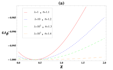
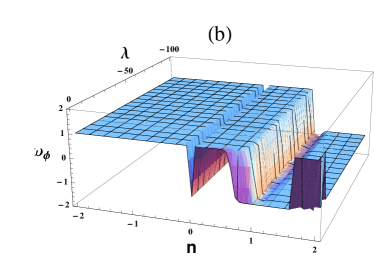
Figure 1: a) The plot of $\omega_{\phi}$ in terms of $z$ and for some values of the parameters $\lambda$ and $n$. There is not any phantom behavior in these cases. b) The plot of $\omega_{\phi}$ for the redshift $z=0.25$. Even though in a small region $\omega_{\phi}$ takes negative values, it does not however cross the PDL.

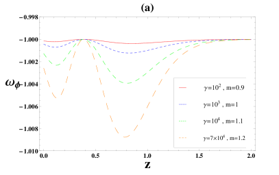
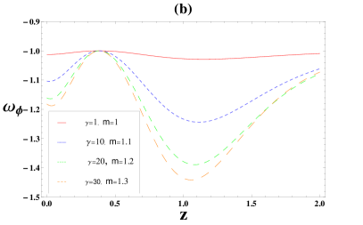
Figure 2: The plot of $\omega_{\phi}(z)$ for (a) Starobinsky’s and (b) Hu-Sawicki’s models. As the figures indicate, there is a phantom-like behavior in the latter.

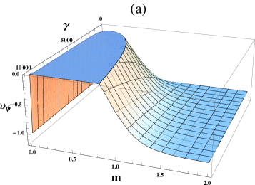
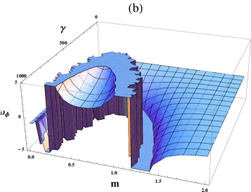
Figure 3: The plot of $\omega_{\phi}$ in the redshift $z=0.25$ for (a) Starobinsky’s and (b) Hu-Sawicki’s models. As the figures show the PDL can be crossed in the latter in a small region of the parameters space.

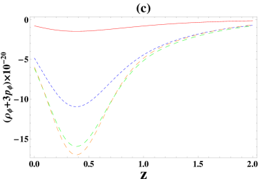
Figure 4: Variations of (a) $\rho_{\phi}$ , (b) $\rho_{\phi}+p_{\phi}$ and (c) $\rho_{\phi}+3p_{\phi}$ in terms of the redshift for Hu-Sawicki’s model. The plots indicate that $\rho_{\phi}<0$ and $\rho_{\phi}+3p_{\phi}<0$ while $\rho_{\phi}+p_{\phi}>0$ for $z<0.4$. The curves are plotted for the same values of the parameters $\gamma$ and $m$ appeared in Fig.2b.

References

-
[1]
A. G. Riess et al., Astron. J. 116, 1009
(1998)
S. Perlmutter et al., Bull. Am. Astron. Soc., 29, 1351 (1997)
S. Perlmutter et al., Astrophys. J., 517 565 (1997) -
[2]
L. Melchiorri et al., Astrophys. J. Letts., 536,
L63 (2000)
C. B. Netterfield et al., Astrophys. J., 571, 604 (2002)
N. W. Halverson et al., Astrophys. J., 568, 38 (2002)
A. E. Lange et al, Phys. Rev. D 63, 042001 (2001)
A. H. Jaffe et al, Phys. Rev. Lett. 86, 3475 (2001) -
[3]
M. Tegmark et al., Phys. Rev. D 69, 103501
(2004)
U. Seljak et al., Phys. Rev. D 71, 103515 (2005) - [4] B. Jain and A. Taylor, Phys. Rev. Lett. 91, 141302 (2003)
- [5] S. M. Carroll, V. Duvvuri, M. Trodden, M. S. Turner, Phys. Rev. D 70, 043528 (2004)
-
[6]
S. M. Carroll,
A. De Felice, V. Duvvuri, D. A. Easson, M. Trodden
and M. S. Turner, Phys. Rev. D 71, 063513 (2005)
G. Allemandi, A. Browiec and M. Francaviglia, Phys. Rev. D 70, 103503 (2004)
X. Meng and P. Wang, Class. Quant. Grav. 21, 951 (2004)
M. E. soussa and R. P. Woodard, Gen. Rel. Grav. 36, 855 (2004)
S. Nojiri and S. D. Odintsov, Phys. Rev. D 68, 123512 (2003)
P. F. Gonzalez-Diaz, Phys. Lett. B 481, 353 (2000)
K. A. Milton, Grav. Cosmol. 9, 66 (2003) - [7] A. G. Riess et al., Astrophys. J. 607, 665 (2004)
-
[8]
U. Alam, V. Sahni, T. D. Saini and A. A. Starobinsky,
Mon. Not. Roy. Astron. Soc. 354, 275 (2004)
S. Nesseris and L. Perivolaropoulos, Phys. Rev. D 70, 043531 (2004) - [9] R. R. Caldwell, Phys. Lett. B 545, 23 (2002)
- [10] R. R. Caldwell, M. Kamionkowski and N. N. Weinberg Phys. Rev. Lett. 91, 071301 (2003)
- [11] K. Bamba, C. Geng, S. Nojiri, S. D. Odintsov, Phys. Rev. D 79, 083014 (2009)
- [12] K. Nozari and T. Azizi, Phys. Lett. B 680, 205 (2009)
- [13] G. Magnano and L. M. Sokolowski, Phys. Rev. D 50, 5039 (1994)
-
[14]
Y. M. Cho, Class. Quantum Grav. 14, 2963
(1997)
E. Elizalde, S. Nojiri and S. D. Odintsov, Phys. Rev. D 70, 043539 (2004)
S. Nojiri and S. D. Odintsov, Phys. Rev. D 74, 086005 (2006)
S. Capozziello, S. Nojiri, S. D. Odintsov and A. Troisi, Phys. Lett. B 639, 135 (2006)
K. Bamba, C. Q. Geng, S. Nojiri and S. D. Odintsov, Phys. Rev. D 79, 083014 (2009)
K. Nozari and S. D. Sadatian, Mod. Phys. Lett. A 24, 3143 (2009) -
[15]
R. J. Scherrer and A. A. Sen, Phys. Rev. D 77, 083515
(2008)
R. J. Scherrer and A. A. Sen, Phys. Rev. D 78, 067303 (2008)
S. Dutta, E. N. Saridakis and R. J. Scherrer, Phys. Rev. D 79, 103005 (2009) - [16] A. Vikman, Phys. Rev. D 71, 023515 (2005)
-
[17]
C. Armendariz-Picon, V. Mukhanov and
P. J. Steinhardt, Phys. Rev. D 63, 103510 (2001)
A. Melchiorri, L. Mersini, C. J. Odman and M. Trodden, Phys. Rev. D 68, 043509 (2003) -
[18]
R. R. Caldwell and M. Doran, Phys.Rev. D 72, 043527
( 2005)
W. Hu, Phys. Rev. D 71, 047301 (2005)
Z. K. Guo, Y. S. Piao, X. M. Zhang and Y. Z. Zhang, Phys.Lett. B 608, 177 (2005)
B. Feng, X. L. Wang and X. M. Zhang, Phys. Lett. B 607, 35 (2005)
B. Feng, M. Li, Y. S. Piao and X. Zhang, Phys. Lett. B 634, 101, (2006) - [19] L. Perivolaropoulos, JCAP 0510, 001 (2005)
-
[20]
A. Linde, JHEP 0111, 052 (2001)
J. Khoury, B. A. Ovrut, P. J. Steinhardt and N. Turok, Phys. Rev. D 64, 123522 (2001)
P. J. Steinhardt and N. Turok, Phys. Rev. D 65, 126003 (2002)
N. Felder, A.V. Frolov, L. Kofman and A. V. Linde, Phys. Rev. D 66, 023507 (2002) - [21] A. de la Macorra and G. German, Int. J. Mod. Phys. D 13, 1939 (2004)
- [22] S. M. Carroll, M. Hoffman and M. Trodden Phys. Rev. D 68, 023509 (2004)
- [23] B. McInnes, JHEP 0208, 029 (2002)
- [24] K. Maeda, Phys. Rev. D 39, 3159 (1989)
- [25] D. Wands, Class. Quant. Grav. 11, 269 (1994)
- [26] Y.G. Gong and A. Wang, Phys. Rev. D 73, 083506 (2006)
- [27] Y. Gong and A. Wang, Phys. Rev. D 75, 043520 (2007)
- [28] S. Capozziello, V. F. Cardone, S. Carloni and A. Troisi, Int. J. Mod. Phys. D 12, 1969 (2003)
- [29] L. Amendola, R. Gannouji, D. Polarski and S. Tsujikawa, Phys. Rev. D 75, 083504 (2007)
- [30] A. A. Starobinsky, JETP. Lett. 86, 157 (2007)
- [31] W. Hu and I. Sawicki, Phys. Rev. D 76, 064004 (2007)