Part I 0

DASTGEER SHAIKH^1,2 B. DASGUPTA² Email:dastgeer.shaikh@uah.eduEmail:brahmananda.dasgupta@uah.edu ¹Department of Physics and
²Center for Space Physics and Aeronomic Research (CSPAR),
University of Alabama at Huntsville, Huntsville, AL 35805. USA.

I–LABEL:lastpage

An analytic model of plasma-neutral coupling in the heliosphere plasma

DASTGEER SHAIKH^1,2 B. DASGUPTA² Email:dastgeer.shaikh@uah.eduEmail:brahmananda.dasgupta@uah.edu ¹Department of Physics and
²Center for Space Physics and Aeronomic Research (CSPAR),
University of Alabama at Huntsville, Huntsville, AL 35805. USA.

Abstract

We have developed an analytic model to describe coupling of plasma and neutral fluids in the partially ionized heliosphere plasma medium. The sources employed in our analytic model are based on a $\kappa$-distribution as opposed to the Maxwellian distribution function. Our model uses the $\kappa$-distribution to analytically model the energetic neutral atoms that result in the heliosphere partially ionized plasma from charge exchange with the protons and subsequently produce a long tail which is otherwise not describable by the Maxwellian distribution. We present our analytic formulation and describe major differences in the sources emerging from these two distinct distributions.

1 Introduction

With the Voyager spacecraft now in the heliosheath (see Fig 1), the in situ character of the solar wind plasma can be explored. Surprisingly, the supersonic solar wind plasma, probed by the ACE/WIND/Cluster spacecrafts near 1 AU (Astronomical Unit), depicts an entirely different character when contrasted with the Voyager I and 2 observations in the heliosheath region (typically beyond 84 AU) (Goldstein et al 1995, Burlaga et al 2005, 2006, 2008, 2009; Stone et al 2005; Decker et al 2005; Richardson et al 2008, Zank 1999). Figure 1 shows an idealized cartoon reflecting our current understanding based on theory, simulations and modeling together with observations. Little is known about the physical processes that govern the intricate multiscale (associated with waves, structures, turbulence) interactions outlined in Fig 1. The supersonic solar wind (SW) plasma interacts with local interstellar medium (LISM) neutral hydrogen (H) gas through charge exchange leading to the creation of energetic pick up ions (PUI). The SW is decelerated, compressed and heated at a shock, the termination shock (TS), across which it develops small scale turbulence (Shukla 1978, Shaikh & Zank 2008, 2010, Shaikh 2010, Shaikh et al 2006, Mendonca & Shukla 2007). In the heliosheath region, the nonlinear structures, such as magnetic hole and humps are found (Burlaga et al 2008, 2009). The SW protons continue to interact with neutrals via charge exchange to produce significant number of pick up ions. Both in the supersonic and subsonic SW (at least in the outer heliosphere) the pressure associated with the PUIs exceeds that of the solar wind protons (Burlaga et al 2009). Both Voyager 1 and 2 are reporting a number of puzzling observations that were not anticipated by existing analytic or simulation models. An intriguing example is that of magnetic field distribution. The latter is lognormal in supersonic solar wind, whereas it exhibits a Gaussian distribution in subsonic heliosheath. Surprisingly, Voyager 2 indicates that the magnetic field distribution is lognormal in the subsonic heliosheath plasma. The source of this apparent discrepancy in the magnetic field distributions reported by Voyagers 1 & 2 in the heliosheath is not known. Another example is that of plasma in heliosheath which is compressed, turbulent and it is an admixture of waves, fluctuations and magnetic structures (magnetic hole/hump, see section 2 for details) (Burlaga 2006, 2009). The effect of PUIs on the formation and evolution of nonlinear magnetic structures, waves and fluctuations in outer heliosphere and the heliosheath plasma are an open question. These issues continue to pose severe challenges to our understanding of the heliosheath plasma.

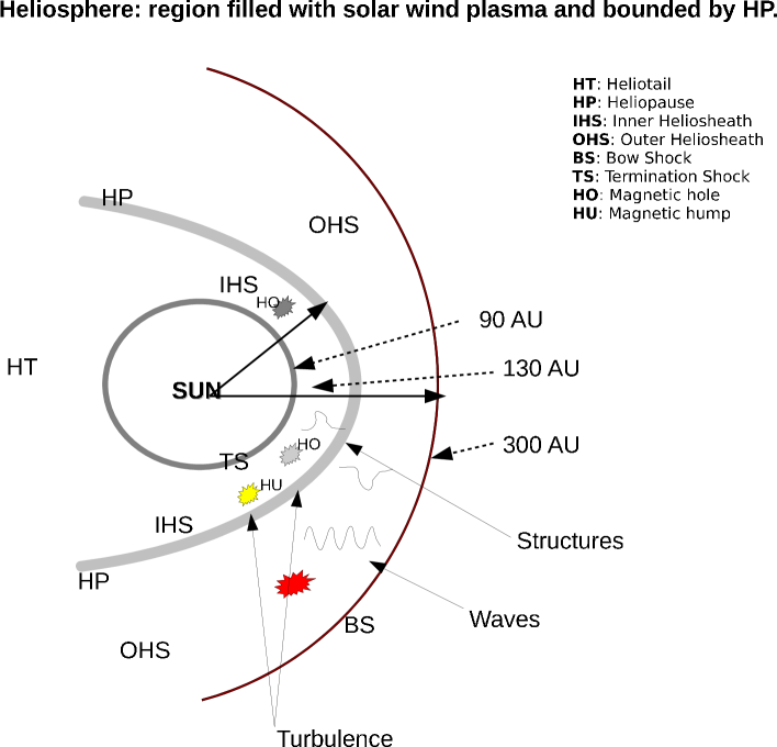
Figure 1: Schematic overview of different regions in the global heliosphere. The solar wind emanating from the Sun propagates outward and interacts with partially ionized interstellar gas predominantly via charge exchange, and creates pick up ions (PUIs). At the termination shock (TS), the supersonic SW decelerated, heated, compressed becoming subsonic, in the heliosheath, and again interacts with interstellar neutrals via charge exchange before it reaches heliopause (HP). The subsonic SW flows down into the heliotail. Magnetic structures such as magnetic holes/humps are observed in heliosheath plasma. During its journey from the Sun to the HP, the solar wind plasma develops multitude of length and time scales that interact with the partially ionized interstellar gas, TS, and nonlinear structures develop in a complex manner.

Although there exists wealth of in situ measurements by the Voyager spacecrafts, they do not provide much information about the global structure of the heliosphere interactions. For instance, the coupling of plasma protons with the interstellar neutral atoms has traditionally been done through Maxwellian sources. However, careful studies have revealed that the distribution of hydrogen neutral (after charge exchanging, they turn into energetic neutral atoms, ENA) does not exactly follow a Maxwellian functions. Recently, Prested et al. (2008) used a $\kappa$-distribution for the ENA parent population to obtain ENA maps. The advantage of using this distribution, as opposed to a Maxwellian, is that it has a power-law tail, and is therefore capable of producing ENA’s at suprathermal energies. Now there has been an increasing consensus that the plasma and neutral fluids follow nearly kappa distribution (Heerikhuisen et al 2008).

A realistic modeling of the heliosheath plasma, one that includes a self-consistent treatment of the PUIs, is therefore critically important and essential to our understanding of the highly variable heliosphere plasma. The central them of this paper is therefore to model complex coupling between plasma and neutral fluids via $\kappa$-distribution as oppose to the Maxwellian distribution. Note here that the $\kappa$ distribution modifies the charge exchange interactions in fluid equations. The kappa-distribution emphasizes charge exchange by high temperature protons. We will investigate the effects of the $\kappa$-distribution in heliosphere plasma turbulence for single fluid plasma-neutral coupled turbulence models.

In section 2, we describe $\kappa$-distribution for neutral and plasma distribution and derive sources for the complex coupling interactions between the two distinct fluids. Section 3 describes complete source terms for the coupling interactions. Finally, a summary is presented in section 5.

2 Plasma neutral coupling via $\kappa$-distribution source

The charge exchange terms can be obtained from the Boltzmann transport equation that describes the evolution of a neutral distribution function $f({\bf r},{\bf v},t)$ in a six-dimensional phase space defined respectively by position and velocity vectors ($x,v_{x},v_{y},v_{z}$) at each time $t$. Here we follow Pauls et al. (1995) in computing the charge exchange terms, based on $\kappa$-distribution functions, from various moments of the Boltzmann equation. The Boltzmann equation for the neutral distribution contains a source term proportional to the proton distribution function $f_{p}$ and a loss term proportional to the neutral distribution function $f_{n}$.

$$\frac{\partial}{\partial t}f_{p}({\bf r},{\bf v},t)+{\bf v}\cdot\nabla f_{p}({\bf r},{\bf v},t)+\frac{{\bf F}}{m}\cdot\nabla_{v}f_{p}({\bf r},{\bf v},t)=$$

$$f_{n}({\bf r},{\bf v},t)\int f_{p}({\bf r},{\bf v_{p}},t)\left|{\bf v_{p}}-{\bf v}\right|\sigma_{ex}(v_{rel})d^{3}{\bf v_{p}}-$$

$$f_{p}({\bf r},{\bf v},t)\int f_{n}({\bf r},{\bf v_{n}},t)\left|{\bf v_{n}}-{\bf v}\right|\sigma_{ex}(v_{rel})d^{3}{\bf v_{n}};$$ (1)

where, $\sigma_{ex}(v_{rel})$ is the charge exchange cross section. The charge exchange parameter has a logarithmically weak dependence on the relative speed ($v_{rel}=|{u}_{p}-{v}_{n}|$) of the neutrals and the protons through $\sigma_{\rm ex}=[(2.1-0.092\ln(v_{rel}))10^{-7}cm]^{2}$ (Fite et al 1962). This cross-section is valid as long as energy does not exceed $1eV$, which usually is the case in the inner/outer heliosphere. Beyond $1eV$ energy, this cross-section yields a higher neutral density. This issue is not applicable to our model and hence we will not consider it here. The density, momentum, and energy of the thermally equilibrated Maxwellian proton and neutral fluids can be computed from Eq. (2) by using the zeroth, first and second moments $\int f_{\xi}d^{3}\xi,\int m{\bf\xi}f_{\xi}d^{3}\xi$ and $\int m\xi^{2}/2f_{\xi}d^{3}\xi$ respectively, where $\xi={u}_{p}$ or ${v}_{n}$. Since charge exchange conserves the density of the proton and neutral fluids, there are no sources in the corresponding continuity equations. We, therefore, need not compute the zeroth moment of the distribution function. Computing directly the first moment from Eq. (2), we obtain the neutral fluid momentum equation.

A similar evolution equation can be written for the neutral distribution function $f_{n}({\bf r},{\bf v_{n}},t)$. We consider the case where both $f_{p}({\bf r},{\bf v_{p}},t)$ and $f_{n}({\bf r},{\bf v_{n}},t)$ are given by a $\kappa$ distribution of the following type:

$$f_{p}({\bf r},{\bf v_{p}})=\frac{n_{p}}{\pi^{\frac{3}{2}}v_{T_{p}}^{3}}\frac{\Gamma(\kappa+1)}{\kappa^{\frac{3}{2}}\Gamma\left(\kappa-\frac{1}{2}\right)}\left[1+\frac{({\bf v_{p}}-{\bf U_{p}})^{2}}{\kappa v_{T_{p}}^{2}}\right]^{-(\kappa+1)};$$ (2)

$$f_{n}({\bf r},{\bf v_{n}})=\frac{n_{n}}{\pi^{\frac{3}{2}}v_{T_{n}}^{3}}\frac{\Gamma(\kappa+1)}{\kappa^{\frac{3}{2}}\Gamma\left(\kappa-\frac{1}{2}\right)}\left[1+\frac{({\bf v_{n}}-{\bf U_{n}})^{2}}{\kappa v_{T_{n}}^{2}}\right]^{-(\kappa+1)}.$$ (3)

First we evaluate the following integral:

$$\beta_{p}({\bf r},{\bf v},t)=\sigma_{ex}(v_{rel})\int f_{p}({\bf r},{\bf v_{p}},t)\left|{\bf v_{p}}-{\bf v}\right|d^{3}{\bf v_{p}};$$ (4)

where $\sigma_{ex}(v_{rel})$ is taken out of the integral, as it varies slowly with respect to $(v_{rel})$. The integral (4) is fully written as

$$\beta_{p}({\bf r},{\bf v},t)=\sigma_{ex}(v_{rel})\frac{n_{p}}{\pi^{\frac{3}{2}}v_{T_{p}}^{3}}A_{\kappa}\int\left[1+\frac{({\bf v_{p}}-{\bf U_{p}})^{2}}{\kappa v_{T_{p}}^{2}}\right]^{-(\kappa+1)}\left|{\bf v_{p}}-{\bf v}\right|d^{3}{\bf v_{p}};$$ (5)

with

$$A_{\kappa}=\frac{\Gamma(\kappa+1)}{\kappa^{\frac{3}{2}}\Gamma\left(\kappa-\frac{1}{2}\right)}.$$

We write,

$${\bf v_{p}}-{\bf U_{p}}=({\bf v_{p}}-{\bf v})-({\bf U_{p}}-{\bf v})$$

and define new variables as

$${\bf V}=({\bf v_{p}}-{\bf v})/\sqrt{\kappa v_{T_{p}}^{2}};\quad{\bf x}=({\bf U_{p}}-{\bf v})/\sqrt{\kappa v_{T_{p}}^{2}};$$

with the new variables, the integral in Eq (5) becomes,

$$\beta_{p}({\bf r},{\bf v},t)=\sigma_{ex}(v_{rel})\frac{n_{p}}{\pi^{\frac{3}{2}}v_{T_{p}}^{3}}(\kappa v_{T_{p}}^{2})^{3/2}\sqrt{\kappa v_{T_{p}}^{2}}A_{\kappa}\int_{-\infty}^{\infty}\left[1+({\bf V}-{\bf x})^{2}\right]^{-(\kappa+1)}Vd^{3}{\bf V};$$ (6)

where we have used,

$$|{\bf v_{p}}-{\bf v}|=\sqrt{\kappa v_{T_{p}}^{2}}V;\quad d^{3}{\bf v_{p}}=(\kappa v_{T_{p}}^{2})^{3/2}d^{3}{\bf V}$$

and the constant before the integral in Eq (6) is,

$$\sigma_{ex}(v_{rel})\frac{n_{p}}{\pi^{\frac{3}{2}}v_{T_{p}}^{3}}(\kappa v_{T_{p}}^{2})^{3/2}\sqrt{\kappa v_{T_{p}}^{2}}~{}\frac{\Gamma(\kappa+1)}{\kappa^{\frac{3}{2}}\Gamma\left(\kappa-\frac{1}{2}\right)}=\sigma_{ex}\frac{n_{p}v_{T_{p}}}{\pi^{\frac{3}{2}}}\frac{\sqrt{\kappa}~{}\Gamma(\kappa+1)}{\Gamma\left(\kappa-\frac{1}{2}\right)}.$$

We now proceed to evaluate the integral Eq (6). In spherical coordinate,

$$d^{3}{\bf V}=V^{2}dv\sin\theta~{}d\theta~{}d\phi,$$

where $\theta$ is the angle between V and x, after performing the $\phi$ integration, with $\mu=\cos\theta$

$$I=2\pi\int^{\infty}_{0}V^{3}dV\int^{1}_{-1}d\mu(1+V^{2}-2Vx\mu+x^{2})^{-(\kappa+1)}$$ (7)

This integration becomes,

$$I=2\left[\int^{x}_{0}z^{2}(1+z^{2})^{-\kappa}dz+x^{2}\int^{x}_{0}(1+z^{2})^{-\kappa}dz+2x\int^{\infty}_{x}z(1+z^{2})^{-\kappa}dz\right],$$

with ${\bf x}=({\bf U_{p}}-{\bf v})/\sqrt{\kappa v_{T_{p}}^{2}}$. We now proceed to determine the explicit values of the above definite integrals. The first two integrals are given in terms of the hypergeometric functions, ${{}_{2}F_{1}}$, which are

$$\int^{x}_{0}z^{2}(1+z^{2})^{-\kappa}dz=\frac{x^{3}}{3}~{}{{}_{2}F_{1}}\left(\frac{3}{2},\kappa;\frac{5}{2};-x^{2}\right),$$

$$x^{2}\int^{x}_{0}(1+z^{2})^{-\kappa}dz=x~{}{{}_{2}F_{1}}\left(\frac{1}{2},\kappa;\frac{3}{2};-x^{2}\right);$$

where the Hypergeometric function ${{}_{2}F_{1}}(a,b;c;z)$ (with $a,b,c$ are constant numbers and $z$ is the variable) is expressed as a power series in $z$:

$${{}_{2}F_{1}}(a,b;c;z) = 1+\frac{ab}{c}\frac{z}{1!}+\frac{a(a+1)b(b+1)}{c(c+1)}\frac{z^{2}}{2!}$$ (8)

$$\quad+\frac{a(a+1)(a+2)b(b+1)(b+2)}{c(c+1)(c+2)}\frac{z^{3}}{3!}+...$$

Using Kummer identity for hypergeometric functions,

$${{}_{2}F_{1}}(a,b;c;z)={{}_{2}F_{1}}(b,a;c;z)=(1-z)^{-b}{{}_{2}F_{1}}[b,c-a;c;z/(z-1)]$$

$${{}_{2}F_{1}}\left(\frac{3}{2},\kappa;\frac{5}{2};-x^{2}\right)=(1+x^{2})^{-\kappa}{{}_{2}F_{1}}\left(\frac{5-3}{2},\kappa;\frac{5}{2};\frac{x^{2}}{1+x^{2}}\right)=(1+x^{2})^{-\kappa}{{}_{2}F_{1}}\left(1,\kappa;\frac{5}{2};\frac{x^{2}}{1+x^{2}}\right);$$

Similarly,

$${{}_{2}F_{1}}\left(\frac{1}{2},\kappa;\frac{3}{2};-x^{2}\right)=(1+x^{2})^{-\kappa}{{}_{2}F_{1}}\left(1,\kappa;\frac{3}{2};\frac{x^{2}}{1+x^{2}}\right)$$

The last integral can be evaluated easily

$$\int^{\infty}_{x}z(1+z^{2})^{-\kappa}dz=\left.\frac{(1+z^{2})^{-\kappa+1}}{2(-\kappa+1)}\right|^{\infty}_{x}=\frac{(1+x^{2})^{-\kappa+1}}{2(\kappa-1)}\quad(\kappa~{}{\rm must~{}be}>1)$$

Collecting the above terms, the integral $\beta_{p}({\bf r},{\bf v})$ is,

$$\beta_{p}({\bf r},{\bf v},t) = \frac{2n_{p}\sigma_{ex}v_{T_{p}}}{\sqrt{\pi\kappa}~{}x}\frac{\Gamma(\kappa+1)}{\Gamma\left(\kappa-\frac{1}{2}\right)}(1+x^{2})^{-\kappa}\left[x^{2}{{}_{2}F_{1}}\left(1,\kappa;\frac{3}{2};\frac{x^{2}}{1+x^{2}}\right)\right.$$

$$+\left.\frac{x^{2}}{3}{{}_{2}F_{1}}\left(1,\kappa;\frac{5}{2};\frac{x^{2}}{1+x^{2}}\right)+\frac{1+x^{2}}{\kappa-1}\right];\quad x=|{\bf U_{p}}-{\bf v}|/\sqrt{\kappa v_{T_{p}}^{2}}$$

An approximate value of the above expression in the two limits $\sqrt{\kappa}~{}x\ll 1$ and $x\gg 1$ can be obtained as follows:

$$\sqrt{\kappa}~{}x\ll 1:\qquad\beta=\frac{2n_{p}\sigma_{ex}v_{T_{p}}}{\sqrt{\pi\kappa}}\frac{\Gamma(\kappa+1)}{\Gamma\left(\kappa-\frac{1}{2}\right)}\left[\frac{1}{\kappa-1}+\frac{({\bf U_{p}}-{\bf v})^{2}}{3\kappa v_{T_{p}}^{2}}\right]$$ (10)

$$x\gg 1:\qquad\beta=n_{p}\sigma_{ex}\sqrt{\frac{4v_{T_{p}}\Gamma^{2}(\kappa+1)}{\pi\kappa(\kappa-1)\Gamma^{2}\left(\kappa-\frac{1}{2}\right)}+({\bf U_{p}}-{\bf v})^{2}}$$ (11)

Note that in an asymptotic limit, the Gamma functions for large argument is

$$\lim_{\kappa\rightarrow\infty}\kappa^{b-a}\frac{\Gamma(\kappa+a)}{\Gamma(\kappa+b)}\rightarrow 1,\quad\Rightarrow\quad\lim_{\kappa\rightarrow\infty}\Gamma(\kappa+a)\simeq\kappa^{a}\Gamma(\kappa)$$

3 Complete expressions for the source terms

To find the source terms, we take the moments of Eq (2) by multipling both sides with various powers of the velocity v. The zeroth order moment would contribute to the source term of the mass continuity equation, the first order moment would contribute to the source term of the momentum equation, the second order moment would contribute to the source term of the energy equation. The moments for the left hand terms of Eq (2) are well known, so we shall show the moments of the right hand terms, using kappa distribution for $f_{p}$ and $f_{n}$. We derive full expression for the integrals on the r.h.s of Eq (2) by using the complete expression for the integral for $\beta_{p}({\bf r},{\bf v},t)$ given by Eq (2) without any approximation.

Since the charge exchange process conserves the proton and neutral density, there will be no source term for the mass continuity term, so we need not calculate the zeroth moment. Hence we start with the first moment of the right hand side of Eq (2). With

$$f_{n}({\bf r},{\bf v})=\frac{n_{n}}{\pi^{\frac{3}{2}}v_{T_{n}}^{3}}\frac{\Gamma(\kappa+1)}{\kappa^{\frac{3}{2}}\Gamma\left(\kappa-\frac{1}{2}\right)}\left[1+\frac{({\bf v}-{\bf U_{n}})^{2}}{\kappa v_{T_{n}}^{2}}\right]^{-(\kappa+1)}=f_{n}({\bf r},{\bf v}-{\bf U_{n}}),$$

$${\rm and}\hskip 64.58313pt\beta_{p}({\bf r},{\bf v},t)\equiv\beta_{p}({\bf r},x,t)=\beta_{p}({\bf r},{\bf U_{p}}-{\bf v})$$

The production term for Momentum transport, is,

$$Q_{MP} = \int_{0}^{\infty}d^{3}v{\bf v}f_{n}({\bf r},{\bf v}-{\bf U_{n}})\beta_{p}({\bf r},{\bf U_{p}}-{\bf v})$$

$$= \int_{0}^{\infty}d^{3}v{\bf U_{n}}f_{n}({\bf r},{\bf v}-{\bf U_{n}})\beta_{p}[{\bf r},({\bf U_{p}}-{\bf U_{n}})-({\bf v}-{\bf U_{n}})]$$

$$+\int_{0}^{\infty}d^{3}v({\bf v}-{\bf U_{n}})f_{n}({\bf r},{\bf v}-{\bf U_{n}})\beta_{p}[{\bf r},({\bf U_{p}}-{\bf U_{n}})-({\bf v}-{\bf U_{n}})],$$

$$= {\bf U_{n}}\int_{0}^{\infty}d^{3}uf_{n}({\bf r},{\bf u})\beta_{p}[{\bf r},(\Delta{\bf U}-{\bf u})]+\int_{0}^{\infty}d^{3}u{\bf u}f_{n}({\bf r},{\bf u})\beta_{p}[{\bf r},(\Delta{\bf U}-{\bf u})];$$

where we used, ${\bf u}={\bf v}-{\bf U_{n}};\quad\Delta{\bf U}={\bf U_{p}}-{\bf U_{n}}$.

The production term for Energy transport, is,

$$Q_{EP} = \int_{0}^{\infty}d^{3}v|{\bf v}|^{2}f_{n}({\bf r},{\bf v}-{\bf U_{n}})\beta_{p}({\bf r},{\bf U_{p}}-{\bf v})$$ (13)

$$= \int_{0}^{\infty}d^{3}v|{\bf v}-{\bf U_{n}}|^{2}f_{n}({\bf r},{\bf v}-{\bf U_{n}})\beta_{p}({\bf r},{\bf U_{p}}-{\bf v})$$

$$+2{\bf U_{n}}\cdot\int_{0}^{\infty}d^{3}v{\bf v}f_{n}({\bf r},{\bf v}-{\bf U_{n}})\beta_{p}({\bf r},{\bf U_{p}}-{\bf v})$$

$$-U_{n}^{2}\int_{0}^{\infty}d^{3}vf_{n}({\bf r},{\bf v}-{\bf U_{n}})\beta_{p}({\bf r},{\bf U_{p}}-{\bf v})$$

$$= \int_{0}^{\infty}d^{3}v|{\bf v}-{\bf U_{n}}|^{2}f_{n}({\bf r},{\bf v}-{\bf U_{n}})\beta_{p}({\bf r},{\bf U_{p}}-{\bf v})$$

$$+2{\bf U_{n}}\cdot\int_{0}^{\infty}d^{3}v({\bf v}-{\bf U_{n}})f_{n}({\bf r},{\bf v}-{\bf U_{n}})\beta_{p}({\bf r},{\bf U_{p}}-{\bf v})$$

$$+2U_{n}^{2}\int_{0}^{\infty}d^{3}vf_{n}({\bf r},{\bf v}-{\bf U_{n}})\beta_{p}({\bf r},{\bf U_{p}}-{\bf v})$$

$$-U_{n}^{2}\int_{0}^{\infty}d^{3}vf_{n}({\bf r},{\bf v}-{\bf U_{n}})\beta_{p}({\bf r},{\bf U_{p}}-{\bf v})$$

As before, we introduce the variables ${\bf u}={\bf v}-{\bf U_{n}};\quad\Delta{\bf U}={\bf U_{p}}-{\bf U_{n}}$ and write $\beta_{p}({\bf r},{\bf U_{p}}-{\bf v})=\beta_{p}({\bf r},({\bf U_{p}}-{\bf U_{n}})-({\bf v}-{\bf U_{n}}))=\beta_{p}({\bf r},\Delta{\bf U}-{\bf u})$. Expression (13) can be written as

$$Q_{EP} = \int_{0}^{\infty}d^{3}uu^{2}f_{n}({\bf r},{\bf u})\beta_{p}({\bf r},\Delta{\bf U}-{\bf u})+2{\bf U_{n}}\cdot\int_{0}^{\infty}d^{3}u{\bf u}f_{n}({\bf r},{\bf u})\beta_{p}({\bf r},\Delta{\bf U}-{\bf u})$$ (14)

$$+U_{n}^{2}\int_{0}^{\infty}d^{3}uf_{n}({\bf r},{\bf u})\beta_{p}({\bf r},\Delta{\bf U}-{\bf u})$$

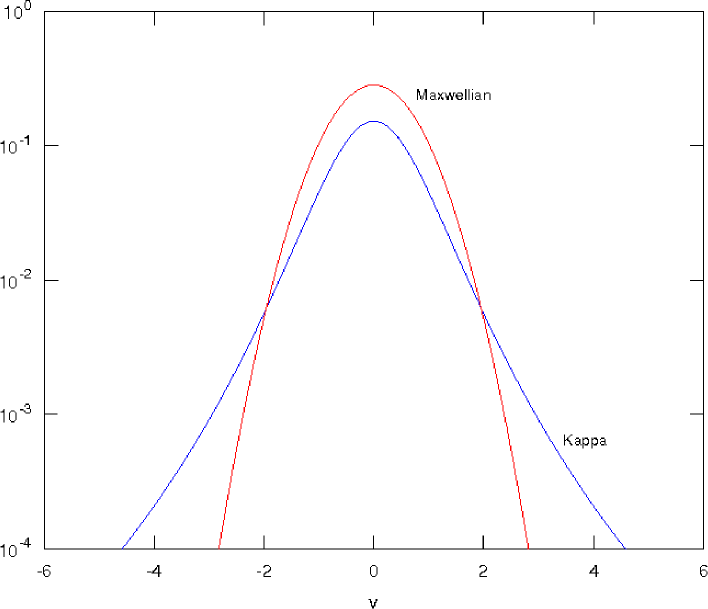
Figure 2: Comparision between the kappa and Maxwellian distribution functions for the sources. Clearly, the tail of the distribution for $\kappa$ function is long and wide as opposed to the Maxwellian distribution. It is because of this feature, we have computed sources based on a $\kappa$-distribution function.

4 Summary and conclusion

In summary, our major results are Eq (3) & Eq (13). A tentative comparison of the sources based on Maxwellian and kappa distribution functions is shown in Fig (2). It is evident from this figure that the sources based on a Maxwellian distribution function falls off sharply and without any tail region. This therefore excludes the energertic component of the neutral atoms and hence is inappropriate for typical ENAs. By contrast, the sources based on a kappa distribution function depicts a well-behaved tail distribution that represents ENA distribution.

Our previous work in Shaikh & Zank (2008) has shown that charge exchange modes modify the helioshperic turbulence cascades dramatically by enhancing nonlinear interaction time-scales on large scales. Thus the coupled plasma system evolves differently than the uncoupled system where large-scale turbulent fluctuations are strongly correlated with charge-exchange modes and they efficiently behave as driven (by charge exchange) energy containing modes of helioshperic turbulence. By contrast, small scale turbulent fluctuations are unaffected by charge exchange modes which evolve like the uncoupled system as the latter becomes less important near the larger $k$ part of the helioshperic turbulent spectrum. The neutral fluid, under the action of charge exchange, tends to enhance the cascade rates by isotropizing the helioshperic plasma turbulence on a relatively long time scale. This tends to modify the characteristics of helioshperic plasma turbulence which can be significantly different from the Kolmogorov phenomenology of fully developed turbulence. It remains to be seen how these modified sources influence nonlinear turbulent properties of the small scale helioshperic plasma fluctuations.

5 Acknowledgment

The partial support of NASA grants NNX09AB40G, NNX07AH18G, NNG05EC85C, NNX09AG63G, NNX08AJ21G, NNX09AB24G, NNX09AG29G, and NNX09AG62G is acknowledged.

19

References

• [1] Burlaga, L. F., N. F. Ness, M. H. Acuna, J. D. Richardson, E. Stone, and F. B. McDonald, The Astrophysical Journal, 692:1125โ€“1130, 2009.
• [2] Burlaga,ย L.ย F. and Ness,ย N.ย F., Astrophysical Journal, 703, 311, 2009.
• [3] Burlaga,ย L.ย F.; Ness,ย N.ย F.; Acuรฑa,ย M.ย H.; Lepping,ย R.ย P.; Connerney,ย J.ย E.ย P.; Richardson,ย J.ย D., Nature, 454, 75, 2008.
• [4] Burlaga, L.F. et al., Science, 309, 2027, 2005.
• [5] Burlaga, L. F.Ness, N. F.;Acuรฑa, M. H., Astrophys. J., 642, 584, 2006.
• [6] Decker, R. B., S. M. Krimigis, E. C. Roelof, M. E. Hill, T. P. Armstrong, G. Gloeckler, D. C. Hamilton, and L. J. Lanzerotti, Science 309, 2020-2024 , 2005.
• [7] Fite, W. L., Smith, A. C. H., and Stebbings, R. F., Proc. R. Soc. London, em A. 268, 527, 1962.
• [8] Goldstein, M. L., Roberts, D. A., andMatthaeus, W. H. Ann. Rev. Astron. & Astrophys., 33, 283, 1995.
• [9] Heerikhuisen,ย J.; Pogorelov,ย N.ย V.; Florinski,ย V.; Zank,ย G.ย P.; leย Roux,ย J.ย A., Astrophysical Journal, 682, 679, 2008.
• [10] Heerikhuisen,ย Jacob; Shaikh,ย Dastgeer; Zank,ย Gary, AIP Conference Proceedings, 932, 123, 2007.
• [11] Mendonca, J. T., and Shukla, P. K., Physics of Plasmas, Volume 14, Issue 12, pp. 122304-122304-4, 2007.
• [12] Pauls, H. L., Zank, G. P., and Williams, L. L., J. Geophys. Res. A11, 21595, 1995.
• [13] Prested, C.; Schwadron, N.; Passuite, J.; Randol, B.; Stuart, B.; Crew, G.; Heerikhuisen, J.; Pogorelov, N.; Zank, G.; Opher, M.; Allegrini, F.; McComas, D. J.; Reno, M.; Roelof, E.; Fuselier, S.; Funsten, H.; Moebius, E.; Saul, L., Journal of Geophysical Research, Volume 113, Issue A6, CiteID A06102, 2008.
• [14] Richardson,ย Johnย D., Plasma Near the Termination Shock and in the Heliosheath, AIPC, 1039, 418, 2008.; Li,ย H.; Wang,ย C.; Richardson,ย J.ย D., Geophysical Res. Lett., 3519107, 2008.
• [15] Shaikh, Dastgeer; Zank, G. P., AIP Conference Proceedings, Volume 1216, pp. 164-167, 2010.
• [16] Shaikh, Dastgeer, Journal of Plasma Physics, In press, 2009arXiv0912.1568S, 2010.
• [17] Shaikh, Dastgeer; Zank, Gary P.; Pogorelov, Nikolai, AIP Conference Proceedings, Volume 858, pp. 308-313, 2006.
• [18] Shaikh, D., and Zank, G. P., The Astrophysical Journal, Volume 688, Issue 1, pp. 683-694, 2008.
• [19] Shukla, P. K., Nature, 274, 874, 1978.
• [20] Zank, G. P., 1999, Space Sci. Rev., 89, 413-688, 1999.