Small-scale behaviour in deterministic reaction models

Abstract

In a recent paper published in this journal [42 (2009) 495004] we studied a one-dimensional particles system where nearest particles attract with a force inversely proportional to a power $\alpha$ of their distance and coalesce upon encounter. Numerics yielded a distribution function $h(z)$ for the gap between neighbouring particles, with $h(z)\sim z^{\beta(\alpha)}$ for small $z$ and $\beta(\alpha)>\alpha$. We can now prove analytically that in the strict limit of $z\to 0$, $\beta=\alpha$ for $\alpha>0$, corresponding to the mean-field result, and we compute the length scale where mean-field breaks down. More generally, in that same limit correlations are negligible for any similar reaction model where attractive forces diverge with vanishing distance. The actual meaning of the measured exponent $\beta(\alpha)$ remains an open question.

1 Introduction

In a recent publication [1] we have studied an infinite system of particles on the line, located at $\{x_{i}(t)\}_{i=-\infty}^{\infty}$, when nearest particles attract one another with a force inversely proportional to a power $\alpha$ of the distance and coalesce upon encounter. In the overdamped limit, we can write

$$\frac{dx_{i}}{dt}=\frac{A}{\alpha}\left(\frac{1}{(x_{i+1}-x_{i})^{\alpha}}-\frac{1}{(x_{i}-x_{i-1})^{\alpha}}\right)$$ (1)

and the gaps between particles, $\ell_{i}=x_{i+1}-x_{i}$, obey

$$\frac{d\ell_{i}}{dt}=\frac{A}{\alpha}\left(\frac{1}{\ell_{i-1}^{\alpha}}-\frac{2}{\ell_{i}^{\alpha}}+\frac{1}{\ell_{i+1}^{\alpha}}\right)\,.$$ (2)

Reacting particles systems such as this, evolving deterministically, occur often enough to merit further study [2, 3, 4, 5, 6, 7, 8]. The case of $\alpha=1$ occurs in the study of crystal growth [2]. For a more detailed discussion see Ref. [1].

In the following we will consider the case of $\alpha>0$, which corresponds to attractive forces that diverge as the gap between nearest particles vanishes. The system is unstable and neigbouring particles tend to attract and coalesce, which leads to a reduction in the number of particles, i.e., to a coarsening process.

Dimensional analysis, as well as a scaling hypothesis applied to the pertinent Fokker-Plank equations, yield the coarsening law [1] for the average distance ${\bar{\ell}}$ between nearest neighbour particles,

$${\bar{\ell}}(t)=[2A(1+\alpha)t]^{n}\,,\qquad n={1/(1+\alpha)}\,.$$ (3)

This firm theoretical result is also strongly supported by unambiguous numerical evidence. In contrast, the distribution function $h(z)$, for the reduced gap $z=\ell/{\bar{\ell}}$ between particles, has proved to be more challenging, both numerically and analytically. In [1] we have presented numerical simulation results supporting a power-law behavior for small $z$,

$$h(z)\sim z^{\beta(\alpha)}\,,$$ (4)

where $\beta(\alpha)>\alpha$: $\beta(0)\approx 1/2$, and $\beta(\alpha)\to\alpha$ as $\alpha\to\infty$ (Fig. 1).

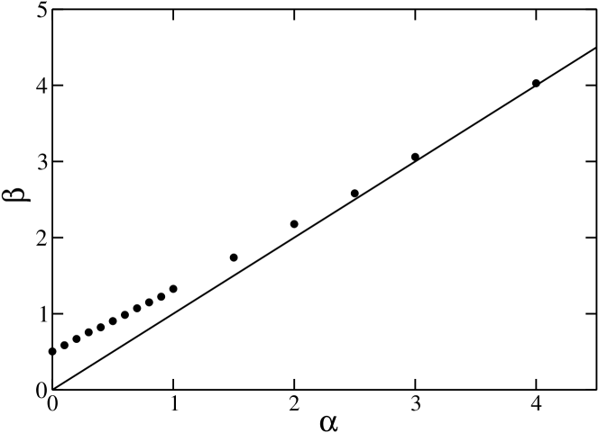
Figure 1: The exponent $\beta$, that describes the small gap behaviour of the gap distribution function, $h(z)\sim z^{\beta}$, as a function of the force exponent $\alpha$, in our deterministic reaction model. The solid line indicates the strict $z\to 0$ limit $\beta=\alpha$ of Eq. (11). After Fig. 1 of Ref. [1].

Analytically, we were unable to do better than mean-field, which predicts $\beta=\alpha$. However, qualitative considerations had suggested that $\beta$ might be larger than $\alpha$, in the presence of sufficiently strong anti-correlations between adjacent gaps.

Below, we show analytically that the exponent $\beta$ and the coarsening exponent $n$ are related to one another. It follows from this relationship that in the strict limit of $z\to 0$, $\beta=\alpha$. The remainder of the paper is devoted to the question of why numerics yield a different value for $\beta$.

2 Relation between the exponents $\beta$ and $n$

Assuming that $\alpha>0$, Eq. (2) tells us that once the gap $\ell_{i}$ is small enough its own size dominates its rate of shrinking and ultimately this rate becomes independent of the neighbouring gaps, $\ell_{i\pm 1}$. Note that $h(z)\to 0$ as $z\to 0$, so the probability that either of the $\ell_{i\pm 1}$ be also small can be safely neglected. Thus, in this limit,

$$\frac{d\ell_{i}}{dt}=-\frac{2A}{\alpha\ell_{i}^{\alpha}}\,,$$ (5)

whose integrations gives

$$\ell_{i}^{\alpha+1}(0)-\ell_{i}^{\alpha+1}(t)=2A\left({\alpha+1\over\alpha}\right)t.$$ (6)

If $\tau$ is the time that it takes for a small gap of size $\ell_{i}(0)=\delta$ to close up, $\ell_{i}(\tau)=0$ (resulting in a coalescence event), we get

$$\delta^{\alpha+1}=2A\left(\frac{\alpha+1}{\alpha}\right)\tau\,.$$ (7)

Suppose that at time $t$ we have $N$ particles. Between $t$ and $t+\tau$ all gaps smaller than $\delta$ would coalesce, so the fraction of coalescence events during the time $\tau$ is equal to the fraction of intervals smaller than $\delta$,

$${dN\over N} = -\int_{0}^{\delta/{\bar{\ell}}}dz\,h(z)=-{B\over\beta+1}\left({\delta\over{\bar{\ell}}}\right)^{\beta+1}$$ (8)

$$= -{B\over\beta+1}{1\over{\bar{\ell}}^{\beta+1}}\left[2A\left({\alpha+1\over\alpha}\right)\tau\right]^{\beta+1\over\alpha+1}\,,$$

where we have assumed the small-$z$ behaviour $h(z)=Bz^{\beta}$ and we have used Eq. (7). On the other hand, since ${\bar{\ell}}=L/N$, where $L$ is the constant, total length of the system, $d{\bar{\ell}}=-{\bar{\ell}}dN/N$, or $dN/N=-d{\bar{\ell}}/{\bar{\ell}}$. Differentiating Eq. (3) for an infinitesimal time $dt=\tau$, we get

$${dN\over N}=-{2A\over{\bar{\ell}}^{\alpha+1}}\tau\,.$$ (9)

We can now equate the right hand sides of Eqs.(8) and (9),

$${B\over\beta+1}{1\over{\bar{\ell}}^{\beta+1}}\left[2A\left({\alpha+1\over\alpha}\right)\tau\right]^{\beta+1\over\alpha+1}={2A\over{\bar{\ell}}^{\alpha+1}}\tau\,,$$ (10)

which must be equal for any small $\tau$. This implies

$$\beta=\alpha\quad{\rm and}\quad B=\alpha\,.$$ (11)

It is worth mentioning that the exponents $n$ and $\beta$ can be related, in principle, following the same procedure as above, also when the attractive force does not diverge with vanishing gap (as for, e.g., an exponential force, $f(\ell)\sim e^{-\ell}$), or when the force is repulsive (our model, with $\alpha<0$). However, in such cases adjacent gaps influence the outcome and correlations are important even in the limit of vanishing $z$, which precludes a simple derivation of $\delta(\tau)$.

3 Correlation effects: discussion and conclusions

Numerically, the observed small-gap exponent, $\beta$, seems to be larger than $\alpha$, the value predicted from the strict limit of $z\to 0$ (Fig. 1). How small need $z$ be for the result $\beta=\alpha$ to hold, even approximately?

Assuming that the small gap $\delta$ is surrounded by gaps of typical length ${\bar{\ell}}$, according to Eq. (2) one can neglect their influence when $1/\delta^{\alpha}\gg{1/{\bar{\ell}}^{\alpha}}$, or

$$\left(\frac{\delta}{{\bar{\ell}}}\right)^{\alpha}<\varepsilon\,,$$ (12)

where $\varepsilon$ is some small positive number representing our error tolerance. We can expect that correlations with adjacent intervals are negligible at (reduced) distances $z<\varepsilon^{1/\alpha}$. This is consistent with the findings of Fig (1) that the error is larger for smaller $\alpha$.

We can make a more accurate assessment of the influence of correlations from neighbouring gaps. Let $h_{2}(z_{1},z_{2})$ be the joint probability density for adjacent gaps of reduced lengths $z_{1}$ and $z_{2}$, and denote by

$$\left\langle 1\over z_{1}^{\alpha}\right\rangle_{z}=\int_{0}^{\infty}dz_{1}{1\over z_{1}^{\alpha}}{h_{2}(z_{1},z)\over h(z)}$$ (13)

the conditional average of $z_{1}^{-\alpha}$, given that the adjacent interval has length $z_{2}=z$. This conditional average obeys the exact expression (Eq. (30), Ref. [1])

$$2\alpha h(z)+\alpha zh^{\prime}(z)=\left[\left(\left\langle\frac{1}{z_{1}^{\alpha}}\right\rangle_{z}-\frac{1}{z^{\alpha}}\right)h(z)\right]^{\prime}\,,$$ (14)

where the prime denotes differentiation with respect to $z$. Numerically, one measures the exponent $\beta$ from the slope of a log-log plot of $h(z)$ vs. $z$. Rearranging (14), we obtain for the local slope:

$$g_{\alpha}(z)=\frac{d(\ln h)}{d(\ln z)}=\frac{zh(z)^{\prime}}{h(z)}=z\frac{-2\alpha+\alpha z^{-\alpha-1}+\left\langle z_{1}^{-\alpha}\right\rangle^{\prime}_{z}}{\alpha z+z^{-\alpha}-\left\langle z_{1}^{-\alpha}\right\rangle_{z}}\,.$$ (15)

Further progress depends on $\left\langle z_{1}^{-\alpha}\right\rangle_{z}$. At the simplest level, mean-field says that $h_{2}(z_{1},z_{2})=h(z_{1})h(z_{2})$, leading to a constant value of the conditional average, which can be shown to be [1]

$$\left\langle{1\over z_{1}^{\alpha}}\right\rangle_{z}=1+\alpha\,.$$ (16)

Another tractable possibility is to assume that adjacent gaps are perfectly anti-correlated: as one interval grows the adjacent gap shrinks, and their total length is fixed, $\ell_{1}+\ell_{2}=2{\bar{\ell}}$, such that $h_{2}(z_{1},z_{2})=h(z_{1})\delta(2-z_{1}-z_{2})$. This leads to

$$\left\langle{1\over z_{1}^{\alpha}}\right\rangle_{z}={1\over(2-z)^{\alpha}}\,.$$ (17)

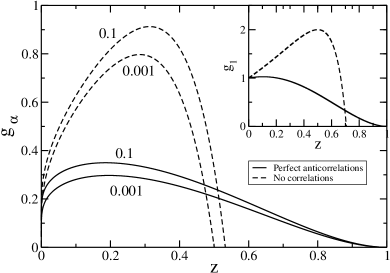
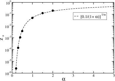
Figure 2: (a) Plot of the local slope $g_{\alpha}(z)$ for $\alpha=0.001$, $0.1$, and $1$ (inset), for the mean-field case (dashed lines) and for perfect correlations (solid lines). (b) The boundary $z_{*}$ within which the mean-field local slope deviates from $\alpha$ by less than $10\,\%$, as obtained numerically from (15) and (16) (symbols) compared to the first-order approximation (18) (dashed line). Note the logarithmic scale.

In Fig. 2a we plot the local slope $g(z)$ for the two assumptions, (16) and (17), for $\alpha=0.001$, $0.1$, and $1$ (inset). In all cases, it is easy to confirm analytically that $g(0)=\alpha$, in agreement with (11). Also evident from the figure, is the fact that $g(z)$ rises sharply near the origin (with infinite slope, for $\alpha<1$), which may explain how numerically one may observe an effective exponent larger than $\alpha$.

We can also use the expression for the local slope, (15), in conjunction with (16), to determine the condition for $\alpha\leq\beta\leq\alpha(1+\varepsilon)$. Solving to first order in $\varepsilon$ we find that $0<z<z_{*}$, with

$$z_{*}\simeq\left({\varepsilon\over 1+\alpha}\right)^{1/\alpha}\,,$$ (18)

(and a similar expression for perfect anti-correlations). Note the similarity to the criterion for neglecting adjacent intervals, derived in the previous section. In Fig. 2b we plot $z_{*}$ for $\varepsilon=0.1$, as a function of $\alpha$. The conclusion is that a change in $\beta$ as big as $10\,\%$ occurs, for most values of $\alpha$, within a very small range of $z$. For example, $z_{*}<10^{-3}$ for $\alpha=0.5$, while the smallest gaps we could analyse using our best numerical data were around $z\approx 0.05$. Clearly, under these conditions one cannot expect to measure the predicted $\beta=\alpha$.

Ultimately, however, the question remains largely open. It is possible, in principle, that when the true correlations are taken into account there exists a fairly wide region of $z>z_{*}$ where the local slope $g(z)\approx\beta>\alpha$ is nearly constant. In that case, the region $0<z<z_{*}$ would be analogous to a boundary layer within which the mean-field result prevails and beyond which a different behaviour sets in.

References

References

- [1] D. ben-Avraham, O. Gromenko and P. Politi, J. Phys. A: Math. Theor. 42, 495004 (2009)
- [2] P. Politi and D. ben-Avraham, Physica D 238, 156 (2009).
- [3] K. Kawasaki, M. C. Yalabik, and J. D. Gunton, Phys. Rev. B 17, 455 (1978); T. Ohta, D. Jasnow, and K. Kawasaki, Phys. Rev. Lett. 49, 1223 (1982).
- [4] I. Ispolatov and P. L. Krapivsky, Phys. Rev. E 53, 3154 (1996).
- [5] A. D. Rutenberg and A. J. Bray, Phys. Rev. E 50, 1900 (1994).
- [6] M. Rost and J. Krug, Physica D 88, 1 (1995).
- [7] See, for example, S. Redner, in Nonequilibrium Statistical Mechanics in One Dimension, V. Privman, ed., (Cambridge University Press, 1997), and references therein.
- [8] B. Derrida, Godreche, and Yekutieli, Phys. Rev. A 44, 6241 (1991).