Anisotropic Mesh Adaptation for Variational Problems
Using Error Estimation Based on Hierarchical Bases

Abstract

Anisotropic mesh adaptation has been successfully applied to the numerical solution of partial differential equations but little considered for variational problems. In this paper, we investigate the use of a global hierarchical basis error estimator for the development of an anisotropic metric tensor needed for the adaptive finite element solution of variational problems. The new metric tensor is completely a posteriori and based on residual, edge jumps and the hierarchical basis error estimator. Numerical results show that it performs comparable with existing metric tensors based on Hessian recovery. A few sweeps of the symmetric Gauß-Seidel iteration for solving the global error problem prove sufficient to provide directional information necessary for successful mesh adaptation.

1 Introduction

Variational problems arise from many areas of science and engineering and have a natural formulation with which the governing equation can be derived through minimization. Often, a variational problem can be transformed into a boundary value problem of partial differential equations (PDEs) and solved by methods specially designed for PDEs. Unfortunately, these methods are not designed to take structural advantage of variational problems and many researches argue that the variational formulation should be used as a natural optimality criterion for mesh adaptation; e.g., see [3, 4, 5]. In this article, we consider mesh adaptation based on the variational formulation.

Most of the existing work for the adaptive numerical solution of variational problems employs isotropic mesh adaptation where the size of mesh elements varies from place to place according to a certain local error estimate while their shape is kept close to equilateral. On the other hand, the ability to allow the size, shape and orientation of mesh elements to vary can significantly improve the accuracy of the solution and enhance the computational efficiency; this is especially true for problems exhibiting distinct anisotropic features. While it has attracted considerable attention from many researchers and been successfully applied to the numerical solution of PDEs, anisotropic mesh adaptation has rarely been employed for variational problems, especially when combined with a posteriori error estimates.

The objective of this article is to investigate the application of a hierarchical basis a posteriori error estimator (HBEE) to anisotropic mesh adaptation for variational problems. We use the $M$-uniform mesh approach [15] where an adaptive mesh is generated as a uniform mesh in the metric specified by a symmetric and strictly positive definite tensor, $M$. The key to the success of the approach is to define a proper metric tensor. Recently, Huang and Li [18] developed a metric tensor for the adaptive finite element solution of variational problems. In the anisotropic case, $M$ is semi-a posteriori: it involves residual and edge jumps, both dependent on the computed solution, and the Hessian of the exact solution, which provides necessary directional information for anisotropic mesh adaptation and is typically approximated using a Hessian recovery technique [18]. On the other hand, an HBEE was used by Huang et al. [17] to develop a metric tensor for the adaptive finite element solution of the boundary value problem of a second-order elliptic differential equation. In this paper we combine the approaches in [17, 18] and develop a metric tensor for variational problems based on an HBEE and the underlying variational formulation. The obtained metric tensor is a posteriori in the sense that it is based solely on residual, edge jumps, and an a posteriori error estimate. This is in contrast to most previous work where $M$ depends on the Hessian of the exact solution and is semi-a posteriori or completely a priori; e.g., see [7, 8, 9, 14, 15, 18]. Numerical results show that the new metric tensor works well for all numerical examples and is comparable in performance with those based on Hessian recovery.

The outline of the paper is as follows. Section 2 is devoted to the description of a general variational problem, its finite element approximation, and the general procedure of the $M$-uniform mesh approach for mesh adaptation. In Section 3, a bound is derived for the variation of the underlying functional. It involves residual, edge jumps, and an HBEE and is minimized on $M$-uniform meshes for an optimal $M$. Numerical examples are given in Section 4. Finally, concluding remarks are given in Section 5.

2 Finite element approximation and mesh adaptation

Consider a general functional of the form

$$I[v]=\int_{\Omega}F(\boldsymbol{x},v,\nabla v)d\boldsymbol{x},\quad\forall v\in U_{0}$$ (1)

where $F(\cdot,\cdot,\cdot)$ is a given smooth function, $\Omega\subset\mathbb{R}^{d}$ ($d=1,2,3$) is the physical domain and $U_{0}$ is a properly selected set of functions satisfying the homogeneous Dirichlet boundary condition

$$v(\boldsymbol{x})=0\quad\forall\boldsymbol{x}\in\partial\Omega.$$

In this paper, we consider only the homogeneous Dirichlet boundary condition. Other boundary conditions can be either converted to the homogeneous Dirichlet boundary condition [13] or treated without major modifications. The corresponding variational problem is to find a minimizer $u\in U_{0}$ such that

$$I[u]=\min_{v\in U_{0}}I[v].$$ (2)

We assume that $F$ satisfies suitable conditions so that the variational problem (2) has a unique solution. We also assume that a linearization of the first variation of the functional (i.e. $B[u;\cdot,\cdot]$, see (3) below) is convex around the solution of the minimization problem. The latter is needed for the error problem (9) defined in Section 3.2 to have a unique solution and for its Gauß-Seidel solution to converge. However, we do not assume that $F$ is quadratic although some theoretical analysis in this paper is valid only for convex quadratic functionals.

A necessary condition for $u$ to be a minimizer is that the first variation of the functional vanishes. This leads to the Galerkin formulation

$$\delta I[u,v]\equiv\int_{\Omega}\left(F_{u}(\boldsymbol{x},u,\nabla u)\;v+F_{\nabla u}(\boldsymbol{x},u,\nabla u)\cdot\nabla v\right)d\boldsymbol{x}=0,\qquad\forall v\in U_{0}$$

where $F_{u}$ and $F_{\nabla u}$ are the partial derivatives of $F$ with respect to $u$ and $\nabla u$, respectively. The linearization of the first variation $\delta I[\cdot,\cdot]$ around the minimizer $u$ with respect to the first argument is given by

$$B[u;w,v]= \int_{\Omega}\left(\frac{}{}v\frac{\partial^{2}F}{\partial u^{2}}(\boldsymbol{x},u,\nabla u)w+v\frac{\partial^{2}F}{\partial u\,\partial\nabla u}(\boldsymbol{x},u,\nabla u)\cdot\nabla w+w\frac{\partial^{2}F}{\partial u\,\partial\nabla u}(\boldsymbol{x},u,\nabla u)\cdot\nabla v\right.$$

$$\left.+\nabla w\cdot\frac{\partial^{2}F}{\partial\nabla u\partial\nabla u}(\boldsymbol{x},u,\nabla u)\cdot\nabla v\frac{}{}\right)d\boldsymbol{x},\qquad\forall w,v\in U_{0}.$$ (3)

Given a triangulation $\mathcal{T}_{h}$ for $\Omega$, let $U_{0}^{h}\subset U_{0}$ be the associated linear finite element space. Then, a linear finite element approximation of $u$ is defined as $u_{h}\in U_{0}^{h}$ such that

$$I[u_{h}]=\min_{v_{h}\in U_{g}^{h}}I[v_{h}].$$

The solution $u_{h}$ can also be found by solving the corresponding Galerkin formulation

$$\delta I[u_{h},v_{h}]=\int_{\Omega}\left(F_{u}(\boldsymbol{x},u_{h},\nabla u_{h})\;v_{h}+F_{\nabla u}(\boldsymbol{x},u_{h},\nabla u_{h})\cdot\nabla v_{h}\right)d\boldsymbol{x}=0,\qquad\forall v_{h}\in U_{0}^{h}.$$ (4)

For the adaptive finite element solution, the mesh $\mathcal{T}_{h}$ is generated according to the behaviour of the error of the approximation $u_{h}$. We follow the so-called $M$-uniform mesh approach [15] with which an adaptive mesh is generated as a uniform mesh in the metric specified by a symmetric and strictly positive definite tensor $M=M(\boldsymbol{x})$. Such a mesh is called an $M$-uniform mesh. A scalar metric tensor will lead to an isotropic mesh while a full metric tensor will generally result in an anisotropic mesh. In this sense, the mesh generation procedure is the same for both isotropic and anisotropic mesh generation. The key to the approach is to choose a proper metric tensor $M$.

Once a metric tensor $M$ has been chosen, a sequence of mesh and corresponding finite element approximation are generated in an iterative fashion. We start with an initial mesh $\mathcal{T}_{h}^{(0)}$. For every mesh $\mathcal{T}_{h}^{(i)}$ we solve the variational problem with $U_{0,(i)}^{h}$ for finite element approximation $u_{h}^{(i)}$. The new mesh $\mathcal{T}_{h}^{(i+1)}$ is generated as an almost $M$-uniform mesh in the metric specified by $M_{h}^{(i)}$ which is computed based on $u_{h}^{(i)}$ and $\mathcal{T}_{h}^{(i)}$. This yields the sequence

$$(\mathcal{T}_{h}^{(0)},U^{h}_{0,(0)})\rightarrow u_{h}^{(0)}\rightarrow M_{h}^{(0)}\rightarrow(\mathcal{T}_{h}^{(1)},U^{h}_{0,(1)})\rightarrow u_{h}^{(1)}\rightarrow M_{h}^{(1)}\rightarrow\cdots$$

The process is repeated until a good adaptation is achieved.

In the following section we derive the metric tensor $M$ for use in anisotropic mesh adaptation for the variational problem (2). First, we derive a bound on the variation $\delta I[u_{h},v]$ and then define $M$ such that the obtained bound is minimized on corresponding $M$-uniform meshes.

3 Monitor functions based on hierarchical basis error estimation

3.1 Error bounds for variational problems

Let $e_{h}=u-u_{h}$ be the error of the finite element solution $u_{h}$. It is known [12] that for a uniformly convex quadratic functional in the form (1), there exists a positive constant $\beta$ such that

$$\|\nabla e_{h}\|_{L^{2}(\Omega)}^{2}\leq\beta\left|\delta I[e_{h},e_{h}]\right|=\beta\left|\delta I[u_{h},e_{h}]\right|.$$

In this case, the quantities

$$\left|\delta I[u_{h},e_{h}]\right|\quad\mbox{and}\quad\left(\frac{|\delta I[u_{h},e_{h}]|}{\|\nabla e_{h}\|_{L^{2}(\Omega)}}\right)^{2}$$ (5)

are equivalent to $\|\nabla e_{h}\|_{L^{2}(\Omega)}^{2}$, and minimizing their bounds is equivalent to minimizing error bounds. Consequently, it is reasonable to define $M$ based on bounds for these quantities even for other functionals.

We begin with deriving a bound for $|\delta I[u_{h},e_{h}]|$. For simplicity we denote

$$F_{u}(\boldsymbol{x})=F_{u}(\boldsymbol{x},u_{h}(\boldsymbol{x}),\nabla u_{h}(\boldsymbol{x})),\quad F_{\nabla u}(\boldsymbol{x})=F_{\nabla u}(\boldsymbol{x},u_{h}(\boldsymbol{x}),\nabla u_{h}(\boldsymbol{x})).$$

Then for any $v\in U_{0}$

$$\delta I[u_{h},v] =\int_{\Omega}\left[F_{u}(\boldsymbol{x},u_{h},\nabla u_{h})\;v+F_{\nabla u}(\boldsymbol{x},u_{h},\nabla u_{h})\cdot\nabla v\right]d\boldsymbol{x}$$

$$=\sum_{K\in\mathcal{T}_{h}}\int_{K}\left[F_{u}(\boldsymbol{x},u_{h},\nabla u_{h})\;v+F_{\nabla u}(\boldsymbol{x},u_{h},\nabla u_{h})\cdot\nabla v\right]d\boldsymbol{x}$$

$$=\sum_{K\in\mathcal{T}_{h}}\int_{K}\left[F_{u}(\boldsymbol{x})\;v+F_{\nabla u}(\boldsymbol{x})\cdot\nabla v\right]d\boldsymbol{x}.$$ (6)

From the divergence theorem, (6) can be rewritten as

$$\delta I[u_{h},v]=\sum_{K\in\mathcal{T}_{h}}\int_{K}\left[F_{u}(\boldsymbol{x})-\nabla\cdot F_{\nabla u}(\boldsymbol{x})\right]\;v\,d\boldsymbol{x}+\sum_{K\in\mathcal{T}_{h}}\int_{\partial{K}}v\;F_{\nabla u}(\boldsymbol{x})\cdot\boldsymbol{n}\,ds,$$ (7)

where $\boldsymbol{n}$ denotes the outward unit normal to the face $\partial K$.

Now, let $\partial\mathcal{T}_{h}$ be the collection of all faces of mesh $\mathcal{T}_{h}$ and $K$ and $K^{\prime}$ be the two elements sharing a common face $\gamma$. We define residual $r_{h}$ and edge jump $R_{h}$ as

$$r_{h}(\boldsymbol{x}) =F_{u}(\boldsymbol{x})-\nabla\cdot F_{\nabla u}(\boldsymbol{x})\qquad\forall\boldsymbol{x}\in K\quad\forall K\in\mathcal{T}_{h},$$

$$R_{h}(\boldsymbol{x}) =\begin{cases}(F_{\nabla u}(\boldsymbol{x})\cdot\boldsymbol{n}_{\gamma})|_{K}+(F_{\nabla u}(\boldsymbol{x})\cdot\boldsymbol{n}_{\gamma})|_{K^{\prime}}&\quad\boldsymbol{x}\in\gamma\quad\forall\gamma\in\partial\mathcal{T}_{h}\backslash\partial\Omega,\\ 0&\quad\boldsymbol{x}\in\gamma\quad\forall\gamma\in\partial\Omega.\end{cases}$$

Then (7) becomes

$$\delta I[u_{h},v]=\sum_{K\in\mathcal{T}_{h}}\int_{K}r_{h}(\boldsymbol{x})\;v\,d\boldsymbol{x}+\sum_{\gamma\in\partial\mathcal{T}_{h}}\int_{\gamma}R_{h}(\boldsymbol{x})\;v\,ds.$$

Taking $v=e_{h}=u-u_{h}$ in the above equation and using Schwarz’s inequality, we obtain

$$\left|{\delta I[u_{h},e_{h}]}\right| \leq\sum_{K\in\mathcal{T}_{h}}\int_{K}\left|{r_{h}(\boldsymbol{x})\;e_{h}}\right|d\boldsymbol{x}+\sum_{\gamma\in\partial\mathcal{T}_{h}}\int_{\gamma}\left|{R_{h}(\boldsymbol{x})\;e_{h}}\right|ds$$

$$\leq\sum_{K\in\mathcal{T}_{h}}\left\|{r_{h}}\right\|_{L^{2}(K)}\left\|{e_{h}}\right\|_{L^{2}(K)}+\sum_{\gamma\in\partial\mathcal{T}_{h}}\left\|{R_{h}}\right\|_{L^{2}(\gamma)}\,\left\|{e_{h}}\right\|_{L^{2}(\gamma)}$$

$$=\sum_{K\in\mathcal{T}_{h}}\left[\left\|{r_{h}}\right\|_{L^{2}(K)}\left\|{e_{h}}\right\|_{L^{2}(K)}+\frac{1}{2}\sum_{\gamma\in\partial K}\left\|{R_{h}}\right\|_{L^{2}(\gamma)}\left\|{e_{h}}\right\|_{L^{2}(\gamma)}\right].$$ (8)

For further derivation, we need to estimate $\left\|{e_{h}}\right\|_{L^{2}(K)}$ and $\left\|{e_{h}}\right\|_{L^{2}(\gamma)}$. In [18], the authors employ anisotropic interpolation error bounds on elements and element faces. This results in a semi-a posteriori metric tensor which involves residual and edge jumps, both dependent on the computed solution, and the Hessian of the exact solution. In the following, we use an a posteriori hierarchical basis error estimate.

3.2 An a posteriori error estimator based on hierarchical bases

The computation of the error estimator is based on a general framework, details on which can be found among others in the work of Bank and Smith [2] or Deuflhard et al. [10]. The approach is briefly explained as follows.

Recall that $u_{h}\in U_{0}^{h}$ is a linear finite element solution of the Galerkin formulation (4) and the error is $e_{h}=u-u_{h}$. Consider the extension of $U_{0}^{h}$ to a subspace of piecewise quadratic functions with the linear span of the edge bubble functions $W^{h}$, i.e.

$$U_{0}^{h}\rightarrow U_{0}^{h}\oplus W^{h}.$$

Recall also that

$$\delta I[u_{h}+e_{h},v]=0\qquad\forall v\in U_{0}.$$

The error estimate $z_{h}$ is then defined as the solution of the approximate linear error problem

$$\begin{cases}\text{Find }z_{h}\in W^{h}\text{ such that}\\ \delta I[u_{h},w_{h}]+B[u_{h};z_{h},w_{h}]=0\quad\forall w_{h}\in W^{h}.\end{cases}$$ (9)

Recall that $B[u_{h};\cdot,\cdot]$ is the bilinear form resulting from the linearization of $\delta I[\cdot,\cdot]$ about $u_{h}$ with respect to the first argument. The estimate $z_{h}$ can be viewed as a projection of the error onto the subspace $W^{h}$. By construction, $\Pi_{h}z_{h}=0$ for the linear finite element interpolation operator $\Pi_{h}$. Thus, $z_{h}-\Pi_{h}z_{h}=z_{h}$.

This definition of the error estimate is global and its solution can be costly. To avoid the expensive exact solution in numerical computation, we employ only a few sweeps of the symmetric Gauß-Seidel iteration for the resulting linear system, which proves to be sufficient for the purpose of mesh adaptation (see [17] or numerical examples in Section 4).

It is noted that under the convex assumption of $B[u;\cdot,\cdot]$, the error problem (9) is solvable and has a unique solution when $u_{h}$ is sufficiently close to $u$. Moreover, Gauß-Seidel iteration is convergent when applied to the solution of (9).

3.3 Optimal metric

We now use the error estimate $z_{h}$ to develop the metric tensor. Instead of directly using the bound (8), we use

$$E[u_{h},z_{h}]=\sum_{K\in\mathcal{T}_{h}}\left[\left\|{r_{h}}\right\|_{L^{2}(K)}\left\|{z_{h}}\right\|_{L^{2}(K)}+\frac{1}{2}\sum_{\gamma\in\partial K}\left\|{R_{h}}\right\|_{L^{2}(\gamma)}\left\|{z_{h}}\right\|_{L^{2}(\gamma)}\right],$$ (10)

which is obtained by replacing $e_{h}$ in (8) with $z_{h}$. Theoretically, it is unclear if the bound (8) is bounded by $E[u_{h},z_{h}]$ although our numerical results show that the metric tensor based on $E[u_{h},z_{h}]$ leads to proper mesh adaptation for all examples we have tested. On the other hand, this is somewhat related to the saturation assumption, which basically states that the quadratic finite element approximation provides a truly better approximation than the linear one. The saturation assumption is known to be valid for some cases under suitable conditions for isotropic meshes [11]. It is still unknown if such results hold for anisotropic meshes.

Recalling that $\Pi_{h}z_{h}=0$ and using element-wise interpolation error estimates in [15], we have

$$\left\|{z_{h}}\right\|_{L^{2}(K)} =\left\|{z_{h}-\Pi_{h}z_{h}}\right\|_{L^{2}(K)}$$

$$\leq C\left[\int_{K}\left(\operatorname{tr}\left((F_{K}^{\prime})^{T}\left|{H(z_{h})}\right|F_{K}^{\prime}\right)\right)^{2}d\boldsymbol{x}\right]^{\frac{1}{2}}$$

$$=C\left|{K}\right|^{\frac{1}{2}}\operatorname{tr}\left((F_{K}^{\prime})^{T}\left|{H_{K}(z_{h})}\right|F_{K}^{\prime}\right),$$ (11)

$$\left[\sum\limits_{\gamma\in\partial K}\frac{1}{\left|{\gamma}\right|}\left\|{z_{h}}\right\|_{L^{2}(\gamma)}^{2}\right]^{\frac{1}{2}} =\left[\sum\limits_{\gamma\in\partial K}\frac{1}{\left|{\gamma}\right|}\left\|{z_{h}-\Pi_{h}z_{h}}\right\|_{L^{2}(\gamma)}^{2}\right]^{\frac{1}{2}}$$

$$\leq C\left[\frac{1}{\left|{K}\right|}\int_{K}\left(\operatorname{tr}\left((F_{K}^{\prime})^{T}\left|{H(z_{h})}\right|F_{K}^{\prime}\right)\right)^{2}d\boldsymbol{x}\right]^{\frac{1}{2}}$$

$$=C\operatorname{tr}\left((F_{K}^{\prime})^{T}\left|{H_{K}(z_{h})}\right|F_{K}^{\prime}\right),$$

where $\operatorname{tr}(\cdot)$ denote the trace of a matrix, $H_{K}(z_{h})$ is the Hessian of $z_{h}$ on $K$, $\left|{H_{K}(z_{h})}\right|=\sqrt{H_{K}^{2}(z_{h})}$, $\left|{K}\right|$ is the volume of $K$, $F_{K}$ is a mapping from the reference element $\hat{K}$ to element $K$, and $C$ is a constant independent of $\mathcal{T}_{h}$ and $z_{h}$. Thus,

$$\sum_{\gamma\in\partial K}\left\|{R_{h}}\right\|_{L^{2}(\gamma)}\left\|{z_{h}}\right\|_{L^{2}(\gamma)} =\sum_{\gamma\in\partial K}\left|{\gamma}\right|^{\frac{1}{2}}\left\|{R_{h}}\right\|_{L^{2}(\gamma)}\left|{\gamma}\right|^{-\frac{1}{2}}\left\|{z_{h}}\right\|_{L^{2}(\gamma)}$$

$$\leq\left(\sum_{\gamma\in\partial K}\left|{\gamma}\right|\left\|{R_{h}}\right\|_{L^{2}(\gamma)}^{2}\right)^{\frac{1}{2}}\left(\sum_{\gamma\in\partial K}\frac{1}{\left|{\gamma}\right|}\left\|{z_{h}}\right\|_{L^{2}(\gamma)}^{2}\right)^{\frac{1}{2}}$$

$$\leq\left(\sum_{\gamma\in\partial K}\left|{\gamma}\right|^{\frac{1}{2}}\left\|{R_{h}}\right\|_{L^{2}(\gamma)}\right)\left(\sum_{\gamma\in\partial K}\frac{1}{\left|{\gamma}\right|}\left\|{z_{h}}\right\|_{L^{2}(\gamma)}^{2}\right)^{\frac{1}{2}}$$

$$\leq C\left(\sum_{\gamma\in\partial K}\left|{\gamma}\right|^{\frac{1}{2}}\left\|{R_{h}}\right\|_{L^{2}(\gamma)}\right)\;\operatorname{tr}\left((F_{K}^{\prime})^{T}\left|{H_{K}(z_{h})}\right|F_{K}^{\prime}\right).$$ (12)

Substituting (11) and (12) into (10) leads to

$$E[u_{h},z_{h}] \leq C\sum_{K\in\mathcal{T}_{h}}\left[\left|{K}\right|^{\frac{1}{2}}\left\|{r_{h}}\right\|_{L^{2}(K)}+\sum_{\gamma\in\partial K}\left|{\gamma}\right|^{\frac{1}{2}}\left\|{R_{h}}\right\|_{L^{2}(\gamma)}\right]\;\operatorname{tr}\left((F_{K}^{\prime})^{T}\left|{H_{K}(z_{h})}\right|F_{K}^{\prime}\right)$$

$$=C\sum_{K\in\mathcal{T}_{h}}\left[\frac{\left\|{r_{h}}\right\|_{L^{2}(K)}}{\left|{K}\right|^{\frac{1}{2}}}+\frac{1}{\left|{K}\right|}\sum_{\gamma\in\partial K}\left|{\gamma}\right|\frac{\left\|{R_{h}}\right\|_{L^{2}(\gamma)}}{\left|{\gamma}\right|^{\frac{1}{2}}}\right]\;\left|{K}\right|\operatorname{tr}\left((F_{K}^{\prime})^{T}\left|{H_{K}(z_{h})}\right|F_{K}^{\prime}\right)$$

$$=C\sum_{K\in\mathcal{T}_{h}}\left[\left\langle{r_{h}}\right\rangle_{L^{2}(K)}+\frac{1}{\left|{K}\right|}\sum_{\gamma\in\partial K}\left|{\gamma}\right|\left\langle{R_{h}}\right\rangle_{L^{2}(\gamma)}\right]\;\left|{K}\right|\operatorname{tr}\left((F_{K}^{\prime})^{T}\left|{H_{K}(z_{h})}\right|F_{K}^{\prime}\right),$$ (13)

where $\left\langle{\cdot}\right\rangle$ denotes the scaled norm

$$\left\langle{v}\right\rangle_{L^{2}(\omega)}=\frac{1}{\left|{\omega}\right|^{1/2}}\left\|{v}\right\|_{L^{2}(\omega)}=\left[\frac{1}{\left|{\omega}\right|}\int_{\omega}v^{2}d\boldsymbol{x}\right]^{\frac{1}{2}}.$$

We now use bound (13) to define the metric tensor $M$. To ensure that $M$ is strictly positive definite, we first regularize the bound with a positive constant $\alpha_{h}$ (to be determined), i.e.,

$$E[u_{h},z_{h}] \leq C\sum_{K\in\mathcal{T}_{h}}\left[\alpha_{h}+\left\langle{r_{h}}\right\rangle_{L^{2}(K)}+\frac{1}{\left|{K}\right|}\sum_{\gamma\in\partial K}\left|{\gamma}\right|\left\langle{R_{h}}\right\rangle_{L^{2}(\gamma)}\right]$$

$$\qquad\qquad\times\left|{K}\right|\operatorname{tr}\left((F_{K}^{\prime})^{T}\left(\alpha_{h}I+\left|{H_{K}(z_{h})}\right|\right)F_{K}^{\prime}\right)$$

$$=C\alpha_{h}^{2}\sum_{K\in\mathcal{T}_{h}}\left[1+\frac{1}{\alpha_{h}}\left\langle{r_{h}}\right\rangle_{L^{2}(K)}+\frac{1}{\alpha_{h}\left|{K}\right|}\sum_{\gamma\in\partial K}\left|{\gamma}\right|\left\langle{R_{h}}\right\rangle_{L^{2}(\gamma)}\right]$$

$$\qquad\qquad\times\left|{K}\right|\operatorname{tr}\left((F_{K}^{\prime})^{T}H_{K,\alpha}(z_{h})F_{K}^{\prime}\right),$$ (14)

where

$$H_{K,\alpha}(z_{h})=I+\frac{1}{\alpha_{h}}\left|{H_{K}(z_{h})}\right|.$$

The optimal metric tensor is obtained by minimizing bound (14) for $M$-uniform meshes. It is known [16] that an $M$-uniform mesh satisfies the alignment condition

$$\frac{1}{d}\operatorname{tr}\left((F_{K}^{\prime})^{T}M_{K}F_{K}^{\prime}\right) =\det\left((F_{K}^{\prime})^{T}M_{K}F_{K}^{\prime}\right)^{\frac{1}{d}}$$ (15)

and the equidistribution condition

$$\rho_{K}\left|{K}\right| =\frac{\sigma_{h}}{N},$$ (16)

where $\sigma_{h}=\sum_{K\in\mathcal{T}_{h}}\rho_{K}\left|{K}\right|$, $M_{K}$ is an average of $M$ over $K$, $\rho_{K}=\sqrt{\det(M_{K})}$, and $N$ the number of elements of $\mathcal{T}_{h}$.

We now pay our attention to the $\mbox{tr}(\cdot)$ factor in (14). Notice that in general,

$$\frac{1}{d}\operatorname{tr}\left((F_{K}^{\prime})^{T}H_{K,\alpha}(z_{h})F_{K}^{\prime}\right)\geq\det\left((F_{K}^{\prime})^{T}H_{K,\alpha}(z_{h})F_{K}^{\prime}\right)^{\frac{1}{d}}.$$

From (15) we can see that the equality in the above inequalities holds if we choose $M=M_{K}$ in the form

$$M_{K}=\theta_{K}H_{K,\alpha}(z_{h})\qquad\forall K\in\mathcal{T}_{h}$$ (17)

for some scalar function $\theta=\theta_{K}$. Indeed, with this choice of $M_{K}$ the alignment condition (15) reads as

$$\frac{1}{d}\operatorname{tr}\left((F_{K}^{\prime})^{T}H_{K,\alpha}F_{K}^{\prime}\right)=\det\left((F_{K}^{\prime})^{T}H_{K,\alpha}F_{K}^{\prime}\right)^{\frac{1}{d}}=\left|{K}\right|^{\frac{2}{d}}\det\left(H_{K,\alpha}(z_{h})\right)^{\frac{1}{d}},$$ (18)

where we have used $\left|{\det(F_{K}^{\prime})}\right|=\left|{K}\right|$ and assumed $|\hat{K}|=1$. Substituting (18) into (14) yields

$$E[u_{h},z_{h}] \leq C\alpha_{h}^{2}\sum_{K\in\mathcal{T}_{h}}\left[1+\frac{1}{\alpha_{h}}\left\langle{r_{h}}\right\rangle_{L^{2}(K)}+\frac{1}{\alpha_{h}\left|{K}\right|}\sum_{\gamma\in\partial K}\left|{\gamma}\right|\left\langle{R_{h}}\right\rangle_{L^{2}(\gamma)}\right]$$

$$\qquad\qquad\times\left|{K}\right|^{\frac{d+2}{d}}\det\left(H_{K,\alpha}(z_{h})\right)^{\frac{1}{d}}.$$ (19)

Next, we use the equidistribution condition (16) to determine $\theta=\theta_{K}$ in (17). From Hölder’s inequality, we have

$$\left[\frac{1}{N}\sum_{K}\left(\left|{K}\right|\rho_{K}\right)^{\frac{d+2}{d}}\right]^{\frac{d}{d+2}}\geq\frac{1}{N}\sum_{K}\left|{K}\right|\rho_{K}=\frac{\sigma_{h}}{N}$$

or

$$\sum_{K}\left(|K|\rho_{K}\right)^{\frac{d+2}{d}}\geq\left({\sigma_{h}}\right)^{\frac{d+2}{d}}N^{-\frac{2}{d}},$$ (20)

with the lower bound being attained for a mesh satisfying (16). Comparing the left-hand side of (20) with the right-hand side of (19) suggests that $\rho=\rho_{K}$ be defined as

$$\rho_{K} =\left[1+\frac{1}{\alpha_{h}}\left\langle{r_{h}}\right\rangle_{L^{2}(K)}+\frac{1}{\alpha_{h}\left|{K}\right|}\sum_{\gamma\in\partial K}\left|{\gamma}\right|\left\langle{R_{h}}\right\rangle_{L^{2}(\gamma)}\right]^{\frac{d}{d+2}}\det\left(H_{K,\alpha}(z_{h})\right)^{\frac{1}{d+2}}$$

$$=\left[1+\frac{1}{\alpha_{h}}\left\langle{r_{h}}\right\rangle_{L^{2}(K)}+\frac{1}{\alpha_{h}\left|{K}\right|}\sum_{\gamma\in\partial K}\left|{\gamma}\right|\left\langle{R_{h}}\right\rangle_{L^{2}(\gamma)}\right]^{\frac{d}{d+2}}\det\left(I+\frac{1}{\alpha_{h}}\left|{H_{K}(z_{h})}\right|\right)^{\frac{1}{d+2}}.$$ (21)

From relations $\rho_{K}=\sqrt{\det(M_{K})}$ and $M_{K}=\theta_{K}H_{K,\alpha}(z_{h})$ we can obtain $\theta_{K}$. The metric tensor $M_{K}$ is then given by

$$M_{K}=\rho_{K}^{\frac{2}{d}}\det\left(I+\frac{1}{\alpha_{h}}\left|{H_{K}(z_{h})}\right|\right)^{-\frac{1}{d}}\left[I+\frac{1}{\alpha_{h}}\left|{H_{K}(z_{h})}\right|\right].$$ (22)

With this choice of $\rho_{K}$ (and $M_{K}$), the right-hand side of (19) attains its lower bound for a mesh satisfying the equidistribution condition (16). Then, the variation of the functional (1) has an upper bound as

$$E[u_{h},z_{h}]\leq C\alpha_{h}^{2}(\sigma_{h})^{\frac{d+2}{d}}N^{-\frac{2}{d}}.$$

To complete the definition of the metric tensor, we need to choose the regularity parameter $\alpha_{h}$. Following [15], we choose it such that

$$\sigma_{h}\equiv\sum_{K\in\mathcal{T}_{h}}\rho_{K}\left|{K}\right|\boldsymbol{=}2\left|{\Omega}\right|$$

or

$$\sum_{K\in\mathcal{T}_{h}}\left|{K}\right|\left[1+\frac{1}{\alpha_{h}}\left\langle{r_{h}}\right\rangle_{L^{2}(K)}+\frac{1}{\alpha_{h}\left|{K}\right|}\sum_{\gamma\in\partial K}\left|{\gamma}\right|\left\langle{R_{h}}\right\rangle_{L^{2}(\gamma)}\right]^{\frac{d}{d+2}}\det\left(I+\frac{1}{\alpha_{h}}\left|{H_{K}(z_{h})}\right|\right)^{\frac{1}{d+2}}$$

$$\qquad=2\left|{\Omega}\right|.$$ (23)

With this choice, roughly fifty percents of the mesh elements will be concentrated in the regions of large $\rho$ [15]. It is easy to show that (23) has a unique solution since its left-hand side is monotonically decreasing with $\alpha_{h}$ increasing and tends to $\left|{\Omega}\right|$ as $\alpha_{h}\to\infty$ and to $+\infty$ as $\alpha_{h}\to 0$. Moreover, it can be solved using a simple iteration scheme such as the bisection method.

Once $\alpha_{h}$ is computed, the adaptation function $\rho$ and the metric tensor $M$ can be determined by (21) and (22), respectively. A new mesh can then be generated based on the metric tensor.

This definition of the metric tensor involves the residual $r_{h}$, the edge jump $R_{h}$, and the HBEE $z_{h}$. All these quantities are based on the computed solution; in this sense, (22) is a posteriori.

4 Numerical results

In this section, we present some numerical results for a selection of two-dimensional problems with an anisotropic behaviour and compare the following metric tensors:

• isotropic a posteriori metric tensor [18] based on the variational formulation, residual, and edge jumps,

• anisotropic semi-a posteriori metric tensor [18] based on the variational formulation, residual, edge jumps, and Hessian recovery,

• anisotropic a posteriori metric tensor based on the variational formulation, residual, edge jumps, and hierarchical basis error estimator (HBEE) developed in the previous section.

The HBEE is computed as a global error problem. A few symmetric Gauß–Seidel iterations are employed to obtain an approximation for $z_{h}$ until the relative difference of the old and the new approximations is under a given tolerance GS-RTOL $=0.01$. More details on several implementation issues such as mesh quality measure and computation of the error estimator can be found in [17, Section 4].

4.1 A quadratic functional

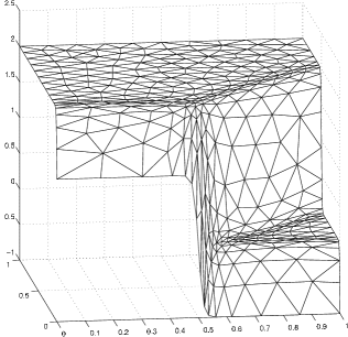
(a) Example 4.1: the exact solution.

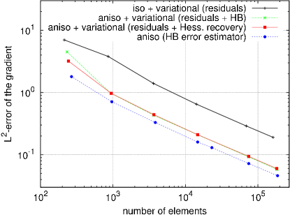
(b) Example 4.1: error comparison.

Figure 1: Example 4.1: LABEL:sub@fig:tanh:plot surface plot of the exact solution, LABEL:sub@fig:tanh:convergence the finite element error $\left\|{\nabla e_{h}}\right\|_{L^{2}(\Omega)}$ against the number of elements.

As a first example we consider a quadratic functional

$$I[u]=\int_{\Omega}\left[\frac{1}{2}\left|{\nabla u}\right|^{2}-uf\right]d\boldsymbol{x}$$ (24)

with $\Omega=(0,1)\times(0,1)$. The function $f$ and the Dirichlet boundary conditions are chosen such that the exact solution of the minimization problem (2) is given by

$$u_{exact}(x,y)=\tanh(60x)-\tanh\left(60(x-y)-30\right).$$

A surface plot of $u_{exact}$ is given in Fig. 1a. The solution exhibits a strong anisotropic behaviour and describes the interaction between a boundary layer along the $x$-axis and a shock wave along the line $y=x-0.5$.

Note that this variational problem is equivalent to the boundary value problem

$$\begin{cases}-\Delta u=f&\text{in }\Omega,\\ u=u_{exact}&\text{on }\partial\Omega.\end{cases}$$

Thus, we also compare metric tensors based on the variational formulation described above with the one based on the hierarchical basis error estimator and PDE developed in [17].

Figure 1b shows $\left\|{\nabla e_{h}}\right\|_{L^{2}(\Omega)}$ (the finite element solution error measured in the $H^{1}$ semi-norm) against the number of elements for all metric tensors; adaptive mesh examples as well as close-up views near the point $(0.5,0)$, where the boundary layer meets the shock wave, are given in Figs. 2 and 3.

Figure 2: Example  4.1 (isotropic): adaptive mesh and a close-up view at (0.5,0) obtained with the isotropic metric tensor based on variational formulation with residual and edge jumps; 664 vertices and 1226 triangles, $\left\|{\nabla e_{h}}\right\|_{L^{2}}=2.8$, maximum aspect ratio 3.

(a) Variational formulation with residual, edge jumps, and Hessian recovery: 663 vertices and 1235 triangles, $\left\|{\nabla e_{h}}\right\|_{L^{2}}=6.2\times 10^{-1}$, maximum aspect ratio 34.

(b) Variational formulation with residual, edge jumps, and HBEE: 672 vertices and 1249 triangles, $\left\|{\nabla e_{h}}\right\|_{L^{2}}=6.0\times 10^{-1}$, maximum aspect ratio 33.

(c) HBEE: 677 vertices and 1256 triangles, $\left\|{\nabla e_{h}}\right\|_{L^{2}}=6.0\times 10^{-1}$, maximum aspect ratio 45.

Figure 3: Example 4.1 (anisotropic): adaptive meshes obtained with different anisotropic metric tensors (left); close-up views at (0.5,0)(right).

First, we observe that all methods provide good mesh density, but anisotropic adaptation (Fig. 3) provides much better mesh alignment with the boundary layer and the shock wave front than isotropic adaptation (Fig. 2). Once again, it shows that anisotropic adaptation is advantageous and should be favored for such problems. Meshes and the solution errors obtained with anisotropic adaptation are very similar. Moreover, mesh adaptation by means of the variational formulation and HBEE is comparable with those obtained with both the Hessian recovery-based method in [18] and the PDE HBEE method in [17].

One may observe that the PDE HBEE method produces a slightly smaller error. The reason for this behaviour can be attributed to the use of the residual and the edge jump in the metric tensor based on the variational formulation: it can be seen as a data smoothing, which prevents the sharp change of the element aspect ratio. The effect can be observed in Fig. 3: the maximum aspect ratio for the metric tensor based on the residual and HBEE is 33 (Fig. 3b), whereas the maximum aspect ratio of the mesh obtained by means of just HBEE is 45 (Fig.  3c). Hence, the PDE HBEE based metric tensor might be a better choice for quadratic functionals with strong anisotropic features.

4.2 A non-quadratic functional

The second example is an anisotropic variational problem [6] defined by the functional

$$I[u]=\int_{\Omega}\left[\left(1+\left|{\nabla u}\right|^{2}\right)^{3/4}+1000u_{y}^{2}\right]d\boldsymbol{x}$$ (25)

with $\Omega=(0,1)\times(0,1)$ and the boundary condition

$$\begin{cases}u=1&\text{on }x=0\text{ or }x=1,\\ u=2&\text{on }y=0\text{ or }y=1.\end{cases}$$

Unlike the previous example, the functional (25) is not quadratic. Hence, the quantities $\left|{\delta I[u_{h},e_{h}]}\right|$ and $\left(\left|{\delta I[u_{h},e_{h}]}\right|/\left|{\nabla e_{h}}\right|_{L^{2}(\Omega)}\right)^{2}$ are not mathematically equivalent to $\left\|{\nabla e_{h}}\right\|^{2}_{L^{2}(\Omega)}$; this example is a good test for the formulas of the metric tensor based on the variational formulation. Analytical solution is not available for this example. A computed solution in Fig. 4 shows that the mesh adaptation challenge for this example lies in the resolution of the sharp boundary layers near $x=0$ and $x=1$.

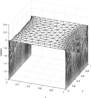
Figure 4: Example 4.2: surface plots of the numerical solutions.

Adaptive meshes obtained with the three different metric tensors (isotropic, Hessian recovery-based, and HBEE-based) are given in Fig. 5. They all have correct mesh concentration, but the anisotropic metric tensors (Figs. 5b and 5c) provide a much better alignment with the boundary layers. Again, both anisotropic meshes are comparable, although mesh elements near the boundary layer in the HBEE-based adaptive mesh have a larger aspect ratio than elements of the mesh obtained by means of the Hessian recovery. This could be due to the smoothing nature of the Hessian recovery: usually, it operates on a larger patch, thus introducing an additional smoothing effect, which affects the grading of the elements’ size and orientation. The global hierarchical basis error estimator does not have this handicap and, in this example, the mesh obtained by means of HBEE is slightly better aligned with the steep boundary layers.

(a) Variational formulation with residual and edge jumps (isotropic): 644 vertices and 1097 triangles, maximum aspect ratio 3.4.

(b) Variational formulation with residual, edge jumps, and Hessian recovery (anisotropic): 649 vertices and 1160 triangles, maximum aspect ratio 15.

(c) Variational formulation with residual, edge jumps, and HBEE: 639 vertices and 1143 triangles, maximum aspect ratio 51.

Figure 5: Example 4.2: adaptive meshes obtained by means of isotropic, anisotropic Hessian recovery-based, and anisotropic HBEE-based metric tensors (left); close-up views at (0,0)(right).

4.3 Image processing

Our third example is an energy functional

$$I[u]=\int_{\Omega}\left[\left(p-u\right)^{2}+\left(1+\left|{\nabla u}\right|^{2}\right)^{1/2}\right]d\boldsymbol{x},$$ (26)

which is used in image processing with the observed image $p$ and the reconstructed image $u$ [1]. In our computation, we choose $\Omega=(0,1)\times(0,1)$,

$$p=1/\left(1+e^{1000(x+y-1.25)}\right)$$

and the boundary condition

$$u=p\quad\text{on }\partial\Omega.$$

The analytical solution is not known; a computed numerical solution is shown in Fig. 6 and Fig. 7 shows examples of adaptive meshes.

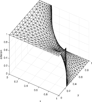
Figure 6: Example 4.3: surface plots of the numerical solution.

(a) Variational formulation with residual and edge jumps (isotropic): 657 vertices and 1207 triangles, maximum aspect ratio 2.7.

(b) Variational formulation with residual, edge jumps, and Hessian recovery (anisotropic): 662 vertices and 1219 triangles, maximum aspect ratio 3.5.

(c) Variational formulation with residual, edge jumps, and HBEE: 656 vertices and 1209 triangles, maximum aspect ratio 4.7.

Figure 7: Example 4.3: adaptive meshes obtained by means of isotropic, anisotropic Hessian recovery-based, and anisotropic HBEE-based metric tensors (left); close-up views at (1,0.25)(right).

As in the previous example, the anisotropic metric tensors are comparable and provide a better mesh adaptation than the isotropic one. Again, the HBEE-based mesh has a slightly larger maximum aspect ratio.

5 Concluding remarks

Numerical results confirm the conclusion of [17] that a global HBEE can be a successful alternative to Hessian recovery in mesh adaptation; a fast approximate solution of the global error problem is sufficient to provide directional information for anisotropic mesh adaptation. They also confirm the conjecture that good mesh adaptation does not require a convergent Hessian recovery or an accurate error estimator, but rather some additional information of global nature, although it is still unclear which information exactly is necessary for successful anisotropic adaptation.

For quadratic functionals, numerical results suggest that algorithms which involve non-directional information such as residual sometime can be slightly disadvantageous for problems with sharp anisotropic features. Such algorithms can smooth out the metric tensor and therefore prevent the rapid change of element size and orientation, which is highly desired for this class of problems. Also, as mentioned in [17], Hessian recovery could result in unnecessarily high mesh density for problems with discontinuities. Global hierarchical error estimation seems less affected by these issues and, depending on the underlying problem, can provide a more robust solution.

Acknowledgment. This work was supported in part by the National Science Foundation (U.S.A.) under grant DMS-0712935 and by the German Research Foundation (DFG) under grant KA 3215/1-1. The authors are grateful to the anonymous referees for their valuable comments.

References

- Aubert and Vese [1997] G. Aubert, L. Vese, A variational method in image recovery, SIAM Journal on Numerical Analysis 34 (1997) 1948–1979.
- Bank and Smith [1993] R.E. Bank, R.K. Smith, A posteriori error estimates based on hierarchical bases, SIAM J. Numer. Anal. 30 (1993) 921–935.
- Becker and Rannacher [1996] R. Becker, R. Rannacher, A feed-back approach to error control in finite element methods: basic analysis and examples, East-West J. Numer. Math. 4 (1996) 237–264.
- Becker and Rannacher [2001] R. Becker, R. Rannacher, An optimal control approach to a posteriori error estimation in finite element methods, Acta Numer. 10 (2001) 1–102.
- Berndt et al. [1997] M. Berndt, T.A. Manteuffel, S.F. Mccormick, Local error estimates and adaptive refinement for first-order system least squares (FOSLS), Electr. Trans. Numer. Anal. 6 (1997) 35–43.
- Bildhauer [2003] M. Bildhauer, Convex variational problems. Linear, nearly linear and anisotropic growth conditions., volume 1818 of Lecture Notes in Mathematics, Springer Berlin / Heidelberg, 2003.
- Borouchaki et al. [1997a] H. Borouchaki, P.L. George, F. Hecht, P. Laug, E. Saltel, Delaunay mesh generation governed by metric specifications. Part I. Algorithms, Finite Elements in Analysis and Design 25 (1997a) 61–83.
- Borouchaki et al. [1997b] H. Borouchaki, P.L. George, B. Mohammadi, Delaunay mesh generation governed by metric specifications. Part II. Applications, Finite Elem. Anal. Des. 25 (1997b) 85–109.
- Castro-Díaz et al. [1997] M.J. Castro-Díaz, F. Hecht, B. Mohammadi, O. Pironneau, Anisotropic unstructured mesh adaption for flow simulations, Int. J. Numer. Meth. Fluids 25 (1997) 475–491.
- Deuflhard et al. [1989] P. Deuflhard, P. Leinen, H. Yserentant, Concepts of an adaptive hierarchical finite element code, Impact Comput. Sci. Engrg. 1 (1989) 3–35.
- Dörfler and Nochetto [2002] W. Dörfler, R.H. Nochetto, Small data oscillation implies the saturation assumption, Numer. Math. 91 (2002) 1–12.
- Evans [1998] L.C. Evans, Partial Differential Equations, volume 19 of Graduate Studies in Mathematics, American Mathematical Society, Providence, Rhode Island, 1998.
- Ern and Guermond [2004] A. Ern, J.-L. Guermond, Theory and Practice of Finite Elements, volume 159 of Applied Mathematical Sciences, Springer-Verlag New York, 2004.
- Frey and George [2008] P.J. Frey, P.L. George, Mesh Generation. Second Edition, John Wiley & Sons, Inc., Hoboken, NJ, 2008.
- Huang [2005] W. Huang, Metric tensors for anisotropic mesh generation, J. Comput. Phys. 204 (2005) 633–665.
- Huang [2006] W. Huang, Mathematical principles of anisotropic mesh adaptation, Commun. Comput. Phys. 1 (2006) 276–310.
- Huang et al. [2010] W. Huang, L. Kamenski, J. Lang, A new anisotropic mesh adaptation method based upon hierarchical a posteriori error estimates, J. Comput. Phys. 229 (2010) 2179–2198.
- Huang and Li [2010] W. Huang, X. Li, An anisotropic mesh adaptation method for the finite element solution of variational problems, Finite Elem. Anal. Des. 46 (2010) 61–73.