The hierarchical build-up of the Tully-Fisher relation

Abstract

We use the semi-analytic model GalICS to predict the Tully-Fisher relation in the B, I and K bands, and its evolution with redshift, up to $z\sim 1$. We refined the determination of the disk galaxies rotation velocity, with a dynamical recipe for the rotation curve, rather than a simple conversion from the total mass to maximum velocity. The new recipe takes into account the disk shape factor, and the angular momentum transfer occurring during secular evolution leading to the formation of bulges. This produces model rotation velocities that are lower by $\sim 30$ km/s in case of Milky Way-like objects, and $\leq 20-30$ km/s for the majority of the spirals, amounting to an average effect of $\sim 20-25\%$. We implemented stellar population models with a complete treatment of the thermally pulsing asymptotic giant branch, which leads to a revision of the mass-to-light ratio in the near-IR. Due to this effect, K band luminosities increase by $\sim 0.5$ at redshift $z=0$ and by $>1$ at $z=3$, while in the I band at the same redshifts the increase amounts to $\sim 0.3$ and $\sim 0.5$ mags. With these two new recipes in place, the comparison between the predicted Tully-Fisher relation with a series of datasets in the optical and near-infrared, at redshifts between 0 and 1, is used as a diagnostics of the assembly and evolution of spiral galaxies in the model. At redshifts $0.4<z<1.2$ the match between the new model and data is remarkably good, expecially for later-type spirals (Sb/Sc). At $z=0$ the new model shows a net improvement in comparison with its original version of 2003, and in accord with recent observations in the K band, the model Tully-Fisher also shows a morphological differentiation. However, in all bands the $z=0$ model Tully-Fisher is too bright. We argue that this behaviour is caused by inadequate star formation histories in the model galaxies at low redshifts. The star-formation rate declines too slowly, due to continuous gas infall that is not efficiently suppressed. An analysis of the model disk scale lengths, at odds with observations, hints to some missing physics in the modeling of disk formation inside dark matter halos.

1 Introduction

The theory of galaxy formation has advanced remarkably in the past decade, thanks to the employment of sophisticated methods of investigation such as numerical simulations and semi-analytic models (see for instance Balland et al. 2003, Baugh et al. 2005, Bower et al. 2006, Cattaneo et al. 2008, Cole et al. 2000, De Lucia et al. 2004, Firmani & Avila-Reese 1999, Hatton et al. 2003, Kauffmann et al. 1993, Menci et al. 2006, Monaco et al. 2007, Somerville et al. 2008, Trujillo-Gomez et al. 2010, van den Bosch 2000, van den Bosch 2002). With these tools, the problem of the assembly of structures in the Universe can be addressed, and the vast number of non-linear physical processes that accompany the formation and evolution of galaxies from primordial perturbations can be modelled.

Interesting for galaxy formation are the observations of scaling relations, that trace a pattern in the assembly history of the vast variety of objects that we observe in the Universe. The origin and nature of such relations is at the core of the mechanism of galaxy assembly (Courteau et al. 2007). One of the most firmly established scaling relations is the Tully-Fisher (hereafter TF; Tully & Fisher, 1977), that correlates the luminosity and the rotation velocity of disk galaxies. The tightness and universality of the relation make it a valid tool to measure extragalactic luminosity distances, since the rotational velocity does not depend on distance or cosmology. But a most interesting aspect of the relation is also the insight it provides on the mechanism of disk assembly (Tonini et al. 2006a).

In the cold dark matter (CDM) scenario for disk galaxy formation (Fall & Efstathiou, 1980), the disk forms out of gas that cools inside a dark matter halo. Initially in equilibrium with the dark matter, the gas collapses into a rotationally supported disk under angular momentum conservation, while the halo evolves adiabatically (Blumenthal et al., 1986). As a consequence, the final equilibrium structure and dynamics of the disk are strongly correlated with those of the dark matter halo, thus providing an insight into the physical halo parameters. In particular, the disk rotation velocity $V_{\rm D}$, the disk size parameterized through the scale-length $R_{\rm D}$, and the disk mass $M_{\rm D}$ are determined by the halo virial properties, $V_{\rm vir}\propto R_{\rm vir}\propto M_{\rm vir}^{1/3}$ (Dutton et al., 2007). The slope of the relation is a function of the radius at which the velocity is measured, mirroring the dark matter mass distribution as a function of galactocentric distance (Yegorova & Salucci, 2007).

Interestingly, although both dynamics and baryonic physics enter the TF, the relation is remarkably tight. In particular, galaxies follow the baryonic TF, which links the dynamical properties of disk (stars $+$ gas) and dark matter halo, with a very small scatter (see for instance McGaugh et al. 2009). In the luminosity $vs$ velocity TF relation, the measured luminosity is given by the stellar emission, and is therefore a proxy for the stellar component. The star formation rate (SFR) and the feedback processes, that regulate the balance between stellar and gas mass, follow a scaling with the dynamical quantities, and provide at the same time a source of scatter.

In galaxy formation models, the supernova feedback efficiency is one of the main parameters driving the slope and zero-point of the TF relation. In fact, being the circular velocity of the disk linked to the halo virial velocity, and therefore to its escape velocity, it is also closely related to the ability of the galaxy to blow a wind. The balance between feedback and star formation sets the amplitude of the TF relation, and its variation across the mass range affects the TF slope (Croton et al. 2006, de Lucia et al. 2004).

Semi-analytic models so far do not have a good grasp of the TF relation. In fact, although both Croton et al. (2006) and de Lucia et al. (2004) reproduce the local I-band TF relation (Giovannelli et al. 1997), this match should not be considered a success because they do not model rotation curves in a physically justified way. De Lucia et al., assumes the total mass profiles are isothermal (i.e., constant circular velocity), while Croton et al. assume the observed rotation velocity is equal to the maximum circular velocity of the dark matter halo (in the absense of galaxy formation). Both of these assumptions are expected to under-predict the true rotation velocities.

On the other hand, semi-analytic models which actually model the galaxy rotation curves do not match the TF relation. Among these, GalICS (Hatton et al. 2003) includes baryons, Cole et al. (2000), Benson et al. (2003) and Benson & Bower (2010) include baryons, NFW halos (Navarro, Frenk & White (1997) and halo contraction.

In addition, it has been pointed out that semi-analytic models cannot simultaneously account for the mass and angular momentum distribution of disk galaxies in a gas-dynamical context (Courteau et al., 2007, van den Bosch et al. 2002b, Governato et al. 2007). In particular for the modeling of the TF relation, sources of systematic errors other than the feedback implementation include the structure of dark matter halos inferred from simulations (the halo concentration and density profile for instance), and the modeling of the dynamics of cooling and baryonic collapse inside halos (see for instance Tonini et al. 2006a, 2006b, Piontek & Steinmetz 2009).

Of interest in the present paper, the predicted TF relation is also affected by the modeling of the galaxy rotational velocity, and the stellar population models implemented. In this work we improve both these recipes in the GalICS model, and re-address the comparison with the observed TF relation. We consider a broad spectral range from the optical to the near-IR, and in particular we perform the comparison in the K band. We also compare the model and observed evolution of the TF up to redshifts $z\sim 1$, both in the optical and in the near-IR.

In current semi-analytic models, the rotation velocity of disk galaxies is a crude estimate based on the virial velocity of the host dark matter halos (for instance de Lucia et al. 2004, Croton et al. 2006), or the sum of a halo $+$ stellar component in spherical symmetry (Hatton et al. 2003). These approximations do not take into account the actual mass profile of the disk, the effects of angular momentum exchange in the galaxy, and the dark matter halo expansion due to dynamical friction, and introduce systematic errors both in the zero-point and in the slope of the predicted TF (see Dutton et al. 2007). In support to this point, Monaco et al. (2007) also showed that the observed baryonic TF relation can be matched by hierarchical models if the dark matter halo concentration is lower than predicted by $\Lambda$CDM simulations (to $c=4$ for halo masses around $10^{12}\ M_{\odot}$).

In the present work, we implement for the first time in the semi-analytic model GalICS (Hatton et al. 2003) a recipe for the galaxy rotation curve that takes into account the shape of the disk and the angular momentum exchange between disk and bulge and between the galaxy and the dark matter halo. We do so by modifying the disk and halo parameters following the recipe proposed by Dutton et al. (2007).

The TF relation predicted by galaxy formation models is also determined by the conversion between stellar mass and light, which is performed through the use of stellar population models. In the original version of GalICS (Hatton et al. 2003) the observed TF relation was not reproduced. In two recent papers (Tonini et al. 2009, 2010) we showed how the predictions of semi-analytic models are greatly affected by the choice of the input stellar populations. In particular we showed how the use of the Maraston (2005; hereafter M05) models allow GalICS to reproduce the colours and near-IR luminosities of $z\sim 2$ galaxies, in the mass and age ranges accessible to hierarchical clustering. In this paper we address the impact of the M05 models on the predicted TF relation in the optical and near-IR, and its evolution with redshift.

This Paper is organized as follows. In Section 2 we introduce the galaxy formation model, and we describe the theoretical recipe to derive the galaxy rotation curves from the dynamical properties of the galaxies and their host dark matter halos, the stellar population models employed, and the method for the selection of model spirals, including the definition of a proxy for the morphological differentiation of these objects. In Section 3 we describe the data samples used to make the comparison between model and observations. In Section 4 we describe the results for the $z=0$ Tully-Fisher, and its dependence on morphology. In Section 5 we address the evolution of the TF with redshift. Finally, in Section 6 we discuss our results and conclude.

2 The model

We produce the model galaxies through the hybrid semi-analytic model GalICS (Hatton et al. 2003), and we defer the reader to its original paper for details on the dark matter N-body simulation and the implementation of the baryonic physics. In brief, the model builds up the galaxies hierarchically, and evolves the metallicity consistently with the cooling and star formation history (with the new implementation of the chemical evolution by Pipino et al., 2009). Feedback recipes for supernovae-driven winds and AGN activity are implemented in the code (the latest with the improved version of Cattaneo et al. 2008). Merger-driven morphology evolution and satellite stripping and disruption are taken into account.

In order to compare the model output with the data, we produce mock galaxy catalogues both in rest-frame and observer-frame, adopting each time the broadband filter sets of the data available for comparison. The broadband magnitudes thus obtained are further scattered with gaussian errors comparable to the observational errors of our data samples (on average $\sigma=0.1$ mag). Dust extinction is treated in the model, however the observed TF relations that we use for the comparison with data are corrected for internal extinction by the various authors. For this reason, we produce unreddened galaxies for the comparison with rest-frame TF relations. When comparing our model galaxies with observed-frame data (not corrected for reddening), we implement dust extinction with a Calzetti extinction curve and a colour-excess $E(B-V)$ proportional to the star formation rate for each single galaxy, parameterized as $E(B-V)=1/3\cdot(\log(SFR)-2)+1/3$ (see Tonini et al. 2010 for a discussion about this choice). Magnitudes are presented in the AB system. We calculate the galaxy rotational velocity at the standard value of $r=2.2R_{\rm D}$ (where $R_{\rm D}$ is the exponential disk scale-length), consistently with the observations used in our comparisons.

The semi-analytic model is rendered for the parameter set $H_{0}=71.9\ \rm km\ s^{-1}\ Mpc^{-1}$, $\Omega_{\Lambda}=0.742$ and $\Omega_{\rm M}=0.258$; these parameters are used to compute observed-frame magnitudes. The model absolute magnitudes are not directly dependent on the cosmology (which obviously enters in the physics of the semi-analytic model, but not in the computation of the rest-frame light emission from galaxies); when comparing with multiple sets of data, analyzed by different authors with various cosmologies, we re-scale all units to the model $h=H_{0}/100$.

2.1 Galaxy rotational velocity

We calculate the rotational velocity of each galaxy by building its rotation curve and evaluating it at $r=2.2R_{\rm D}$, where $R_{\rm D}$ is the disk scale-length. Galaxies in the models are systems composed of a dark matter halo and stars distributed in a disk and a bulge; neglecting the gas component (which is not dominant in mass, at least at $z<1$) the rotation curve is

$$V_{\rm rot}^{2}(r)=V^{2}_{\rm H}(r)+V^{2}_{\rm disk}(r)+V^{2}_{\rm bulge}(r)~{},$$ (1)

with $r$ being the galactocentric distance. For the spheroidal components, i.e. the halo and the bulge, the contribution to the velocity is simply $V^{2}(r)=\sqrt{GM(r)/r}$. Following the original GalICS recipe, the halo density profile is defined as a truncated isothermal sphere. In the simulation halos are tidally truncated by the surrounding density field, and the inner region of halos is virialized. For the purpose of building the rotation curves, we consider halos as spherically symmetric isothermal spheres out to the virial radius. In addition, halos have a finite density core to avoid the singularity. The density profile can be parameterized as follows:

$$\rho(r)=\frac{\rho_{0}}{\left(\frac{r}{r_{\rm S}}\right)^{\gamma}\left[1+\left(\frac{r}{r_{\rm S}}\right)^{1/\alpha}\right]^{\alpha(\beta-\gamma)}}~{},$$ (2)

with $(\alpha,\beta,\gamma)=(1,2,0)$. Fits to the radial mass distrubution of halos in dark matter-only N-body simulations produce the NFW density profile (NFW 1997), which belongs to the same family of functions, with parameters $(1,3,1)$. At intermediate radii NFW halos and isothermal spheres have the same density profile, while at the centre the NFW is shallower and at the outskirts it is steeper. However, in the range of galactocentric distances of interest in the present work, the difference between the two profiles is negligible (as is illustrated later on in this Section). In general, the choice of the halo functional form is a source of uncertainty, and it should be noted that there is an ongoing debate in the literature regarding the shape of dark matter halos in the presence of baryons, expecially in the center of galaxies where the dark matter component reacts to baryonic mass assembly with either expansion or contraction (see for instance Tonini et al. 2006b, Duffy et al. 2010).

The halo is almost entirely pressure-supported, with a mild spin component, parameterized by $\lambda=J|E|^{1/2}/GM_{H}^{5/2}$ in terms of the halo total mass $M$, angular momentum $J$ and binding energy $E$. In simulations the distribution of the halo spin parameter appears to be log-normal, with both median and scatter independent of mass and redshift to a good approximation (see e.g. Bullock et al. 2001, Vitvitska et al. 2002, Hetznecker & Burkert 2006, Bett et al. 2007, Maccio et al. 2007). The median spin parameter for GalICS relaxed halos is $\lambda\sim 0.04$. For each galaxy in GalICS, all halo parameters (virial mass and radius, and velocity dispersions) are directly taken from the N-body simulation, and naturally cause some scatter in the halo profile.

The bulge stellar mass distribution follows a Hernquist (1990) profile, characterized by parameters $(1,4,1)$, and is assumed to be entirely pressure-supported (see Hatton et al. 2003 for details on bulge formation and geometry).

The disk structure and rotation is determined by the halo spin parameter $\lambda$ following Mo et al. (1998). The disk forms from a baryonic gaseous component that initially has the same specific angular momentum as the halo, a mass $m_{\rm D}$ in units of the halo mass, and a total angular momentum $j_{\rm D}$ in units of the halo angular momentum. The disk is assumed to have an exponential surface density profile, with a scale-length defined as:

$$R_{\rm D}=\frac{1}{\sqrt{2}}\left(\frac{j_{\rm D}}{m_{\rm D}}\right)\lambda R_{\rm H}~{},$$ (3)

where $R_{\rm H}$ is the halo virial radius (see Mo et al. 1998 for details). In galaxy formation models the assumption of specific angular momentum conservation during disk formation is widely used, which leads to $j_{\rm D}/m_{\rm D}=1$. This assumption, while useful to semplificate the problem and avoid additional degrees of freedom, is often unrealistic. In fact, angular momentum transfer from the infalling baryons to the halo pushes the ratio lower than unity, and both the halo and the disk structure are be affected (see Tonini et al. 2006b; also, Piontek & Steinmetz 2009). On the other hand, the ratio can also become greater than unity in case of removal of low angular momentum material (e.g., Maller & Dekel 2002, Dutton & van den Bosch 2009). A discussion on the disk sizes of the model galaxies is to be found in the last Section.

In the Hatton et al. (2003) version of GalICS, the disk component of the velocity was treated as $V^{2}(r)=\sqrt{GM(r)/r}$ (for future reference, this will be called the ’spheroidal’ velocity model). However, neglecting the shape factor in the disk gravitational potential leads to an underestimation of the maximum rotational velocity by about $15\%$, under angular momentum conservation (Binney & Tremaine, 2008). For the disk component, in order to take into account the shape factor we assume that

$$V^{2}_{\rm disk}(r)=\frac{GM_{\rm D}}{2R_{\rm D}}\ \left(\frac{r}{R_{\rm D}}\right)^{2}[I_{\rm 0}K_{\rm 0}-I_{\rm 1}K_{\rm 1}]_{r/2R_{\rm D}}~{},$$ (4)

where $M_{\rm D}$ is the total disk mass, and $I,K$ are modified Bessel functions of first and second kind (Tonini et al. 2006, Salucci et al. 2007). This recipe effectively increases the rotational velocity of disk-dominated systems, and has therefore an effect on the TF relation expecially at the high-mass end. For future reference, we call $V_{\rm disky}$ the total rotational velocity when $V^{2}_{\rm disk}$ is modeled as in Eq. (4).

Angular momentum conservation is not a realistic scenario also during bulge formation, as pointed out by Dutton et al. (2007). When bulges form through disk instabilities, part of the material in the disk loses its angular momentum, leading to the formation of a pressure-supported component at the center. The lost angular momentum is transferred to the rest of the disk and the dark matter halo, as seen in numerical simulations (Hohl 1971, Debattista et al. 2006). This affects the value of $R_{\rm D}$ through $j_{\rm D}/m_{\rm D}$ after bulge formation. Following Dutton et al. (2007), after defining $\Theta=M_{\rm bulge}/M_{\rm disk}$, the new disk scale-length is

$$R_{\rm D}=\frac{1}{\sqrt{2}}f_{\rm R}\ f_{\rm H}[1+(1-f_{\rm x})\Theta]\left(\frac{j_{\rm D}}{m_{\rm D}}\right)\lambda R_{\rm H}~{};$$ (5)

the quantity $f_{\rm x}$ expresses the ratio between the specific angular momentum lost by the disk to the halo during bulge formation, to the total specific angular momentum of the baryonic material that went to form disk and bulge. We re-calculate the disk scale-lengths of the galaxies in the simulation with this new recipe, obtaining

$$R_{\rm D_{\rm new}}=R_{\rm D_{\rm MMW}}\left(1+(1-f_{\rm x})\frac{M_{\rm bulge}}{M_{\rm disk}}\right)~{},$$ (6)

and we use the fiducial value $f_{\rm x}=0.25$ indicated by Dutton et al. (2007). By inserting this new value of $R_{\rm D}$ into Eq. (4), we obtain what we will refer to as the ’new’ model for the total rotational velocity, $V_{\rm new}$, from Eq. (1).

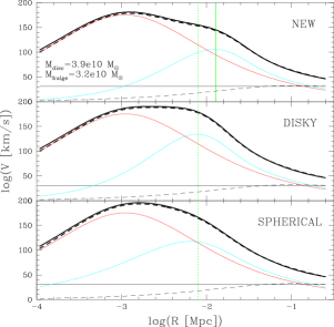
Figure 1: Rotation curve of a simulated galaxy at $z=0$, with disk mass $M_{\rm disk}=3.9\ 10^{10}\ M_{\odot}$ and bulge mass $M_{\rm bulge}=3.2\ 10^{1}0\ M_{\odot}$. The ’new’, ’disky’ and ’spheroidal’ models for the rotation curve are compared (from upper to lower panel). The vertical dotted green line shows the radius $r=2.2R_{\rm D}$ before including the angular momentum transfer from bulge to disk. In the upper panel, the vertical solid green line shows the new location of $r=2.2R_{\rm D}$ after angular momentum transfer. In all panels, solid thick black lines show the total rotation curve, solid blue lines show the disk component of the velocity, solid red lines show the bulge component. The solid thin black lines show the halo component as a truncated isothermal sphere, while the dashed thin black lines show the halo contribution as an NFW profile. The dashed thick black lines show the total rotation curve if the halo is an NFW.

.

Fig. (1) shows the comparison between the three models for the rotation curve, ’new’, ’disky’ and ’spheroidal’ (panels from upper to lower, respectively), for a simulated galaxy at $z=0$, which was chosen for the conspicuous bulge ($M_{\rm bulge}=3.2\ 10^{1}0\ M_{\odot}$ and $M_{\rm disk}=3.9\ 10^{10}\ M_{\odot}$). In all panels, the vertical dotted green line shows the radius $r=2.2R_{\rm D}$ before the evaluation of the angular momentum transfer from bulge to disk. In the upper panel, the new value of $r=2.2R_{\rm D}$ following the angular momentum transfer (’new’ model) is shown as a vertical solid green line. In all panels, solid thick black lines show the total rotation curve, solid blue lines show the disk component of the velocity, solid red lines show the bulge component.

Note that, for a pure disk, the peak of the rotation curve is always approximately at $r=2.2R_{\rm D}$ (making this particular radius the favourite in observations). From the ’spheroidal’ to the ’disky’ model, the disk component of the velocity features a more distinguished peak, with the result that the maximum of the total rotation curve is closer to $r=2.2R_{\rm D}$, and the bulge is less prominent in determining its value. The sharpening of the disk peak causes the measured total velocity to increase.

However, the presence of other mass components, such as the bulge and the halo, tend to broaden the total velocity peak and push it to smaller radii, where these components are more concentrated. But the concentration of the bulge mass at the expense of the disk must be accompanied by angular momentum transfer from the bulge to the disk itself, and according to Eq. (6), the higher the ratio $M_{\rm bulge}/M_{\rm disk}$, the more the disk scale-lenght consequently increases, leading to the ’new’ model and a re-distribution of the disk mass. The disk expands radially and, since it conserves its mass, it becomes less dense. Its velocity peak broadens and it is pushed outwards, thus stretching the total rotation curve. Due to the decreased density, the disk potential well is lower, and this, together with the rapidly declining bulge contribution, lowers the total velocity measured at the new $r=2.2R_{\rm D}$. Since this effect if brought about by the presence of the bulge, it is going to be expecially important at the high-mass end of the model TF relation, where bulge formation is more frequent (this is a feature of the hierarchical model which will be discussed later on).

In Fig. (1) we also show the halo component of the total rotation curve. The thin solid black line is the velocity profile of the truncated isothermal sphere, while the thin dashed black line is the velocity profile of the NFW halo of same virial parameters. The total rotation curve obtained with the NFW (thick solid black lines) is virtually undistinguishable from the one obtained with the truncated isothermal sphere (solid thick black lines), expecially around the region $r=2.2R_{\rm D}$ and beyond.

The new recipe for the rotation velocity allows for a sharper differentiation of the model rotation curves depending on the galaxy morphology, a fact that has been long since observed in nature (Salucci et al. 2007). In particular, in the upper panel of Fig. (1) the bump in the rotation curve due to the presence of the bulge component is clearly visible.

The velocity recipe can be further optimized if one takes into account the dark matter halo evolution triggered by the formation of the galaxy. As proposed in Tonini et al. (2006b) and discussed in Dutton et al. (2007), angular momentum exchange between the collapsing baryonic component and the dark matter causes halo expansion, which affects the halo structural shape and ultimately the dark matter contribution to the rotation curve. However, such a recipe would require more fundamental modifications to the prescriptions for the dark matter halos in the semi-analytic code, and is beyond the scope of this paper.

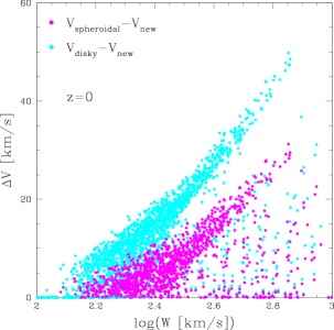
Figure 2: The difference in the predicted $z=0$ galaxy rotational velocity at $r=2.2R_{\rm D}$ with different assumptions for the disk velocity, as a function of the total ’new’ rotation velocity. Magenta points: difference between the original Hatton et al. (2003) model and the ’new’ model. Cyan points): difference between the ’disky’ model and the ’new’ model presented here. For each of the models, we plot the total velocity difference $\Delta V$ against the quantity $log(W=2V_{\rm rot})$, which is used for the comparison with observations later on.

Fig. (2) illustrates the difference in the predicted total rotational velocity (at $z=0$) at the radius $r=2.2R_{\rm D}$ between the ’new’ velocity model and the ’spheroidal’ model (magenta dots), and between the ’new’ model and the ’disky’ model (cyan dots), as a function of $log(W=2V_{\rm new})$, which is used for the comparison with observations later on.

The combined effect of increasing the disk scale-lenght and decreasing the bulge contribution to the rotation curve, is that the ’new’ model velocity is always lower than the ’spheroidal’ model velocity, with a difference up to $\sim 30$ km/s at the high-mass end. On the other hand, the ’new’ model velocity is also always lower than the ’disky’ model velocity, by up to $\sim 50$ km/s at the high-mass end, where bulges contribute significantly to the stellar mass. The difference $\Delta V$ correlates in fact strongly with the total mass, and tends to zero for galaxies with small bulges.

With the new recipe in place, model rotation velocities are lower by $\sim 20-30$ km/s or less, compared to the ’spheroidal’ model, for spirals less massive than the Milky Way, and by $\sim 40-50$ km/s for Milky Way-like objects.

In what follows, we adopt the ’new’ model to compare the model predictions with the data.

2.2 Stellar population models

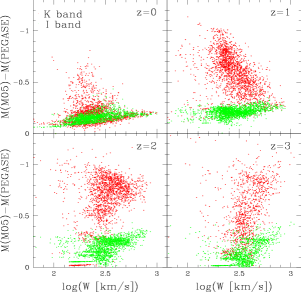
Figure 3: Difference between the predicted rest-frame TF in the M05 and PEGASE runs, as a function of redshift. The green dots show the I band and the red dots show the K band.

The photometry of the model galaxies is produced with the use of the M05 stellar population models, which include a detailed treatment of the Thermally Pulsing Asymptotic Giant Branch phase of stellar evolution. The implementation of the M05 stellar populations in the semi-analytic model significantly improves the predictions for the colours and near-IR luminosities of galaxies, expecially at high redshift. The comparison of the model performance when equipped with the M05 and with its original input stellar populations (PEGASE, Fioc & Rocca-Volmerange, 1997) shows that the inclusion of the TP-AGB produces near-IR luminosities more than 1 magnitude brighter for a given stellar mass, and $V-K$ colours more than 1 magnitude redder, matching the observations of high-redshift galaxies (Tonini et al. 2009, 2010, Henriques et al. in prep.).

The TP-AGB light emission starts at wavelengths $\lambda>5000\ \mathring{A}$, peaks in the rest-frame K band, and affects the nearby bands from the red part of the optical spectrum down to the infrared. This affects both the zero-point and the slope of the predicted TF relation, as a function of redshift. Fig. (3) shows the difference in magnitude between the TF relation predicted with the M05 and the PEGASE runs of the semi-analytic model, in the rest-frame I band (green dots) and K band (red dots), in four redshift bins from 0 to 3. On the $x-$axis we plot $W=2V_{\rm rot}$. The difference between the M05 and PEGASE TF in the I band tends to mildly increase with increasing redshift. The median magnitude difference in the redshift bins centered in $z=0,1,2,3$ is respectively $\Delta(TF)\sim 0.15,0.22,0.25,0.2$ mags. At $z=2,3$ there is a mild dependence with galaxy mass, so that the difference can go up to $\Delta(TF)\sim 0.35-0.4$ for massive galaxies. In the K band, we find a significant increase of the difference $\Delta(TF)$ with redshift. In the redshift bins centered in $z=0,1,2,3$ we find the median $\Delta(TF)\sim 0.2,0.65,0.8,0.7$ mags with maximum $\Delta(TF)>1$ mags for $z\geq 1$. There is no significant trend with galaxy mass.

From now on in this work, the M05 models will be used for all the comparison with data.

2.3 Selection of model galaxies

The determination of the morphology of the model galaxies is based on the relative contribution of bulge and disk to some galactic property, and can be carried about in various ways. For the purpose of a more comprehensive study, we adopted two different criteria for the selection of the model spiral galaxies.

Hatton et al. (2003) defined as spiral galaxies the objects for which the ratio between the bulge and disk luminosity in the B band did not exceed a given threshold. Simien & de Vaucouleurs (1986) found that this ratio correlates well with the Hubble type (see for instance Graham & Worley 2008 for an updated study). Following this criterium, if we define the parameter $\gamma=exp(-L_{\rm bulge}/L_{\rm disk})$, the objects with $\gamma>0.507$ are defined as spirals (see also Baugh et al. 1996). This classification has the advantage to be observationally-oriented, but it depends on the spectrophotometric model in use (including dust reddening), and yields no dynamical information.

From the semi-analytic model point of view, we have the information about the mass and size of disk and bulge before we compute the stellar emission, so we can also classify our galaxies directly in terms of the ratio between the bulge and disk stellar mass, to mimic the morphological differentiation. We choose to split our galaxies in 5 subsamples, defined by $M_{\rm bulge}/M_{\rm disk}$ in 5 intervals: galaxies with $M_{\rm bulge}/M_{\rm disk}<0.25$ loosely correspond to Sc/Irregulars, galaxies with $0.25<M_{\rm bulge}/M_{\rm disk}<0.5$ loosely correspond to Sb spirals, galaxies with $0.5<M_{\rm bulge}/M_{\rm disk}<0.75$ loosely correspond to Sa spirals, and galaxies with $0.75<M_{\rm bulge}/M_{\rm disk}<1$ are similar to ’S0’ types. Strictly speaking, observed S0 galaxies are not identified depending on the bulge/disk mass ratio, but are rather selected to be passively evolving disks, based on colours. Our morphology selection does not depend on photometry, but nonetheless it naturally preserves the correspondence between bulges and old stellar populations, since bulges in the model do not form new stars (except in merger events).

We find that our somewhat arbitrary selection criterium qualitatively matches the observed properties of spirals (K. Masters, private communication). It is also consistent with other prescriptions used in the literature: we re-selected our Sb/Sc spirals following both Croton et al. (2006) and de Lucia et al. (2004), and found that the resulting subsample coincides with the one selected in terms of $M_{\rm bulge}/M_{\rm disk}$. The totality of the spirals in the range $0<M_{\rm bulge}/M_{\rm disk}<1$ is almost coincident with the sample selected with the Hatton et al. (2003) criterium (with the exception of some massive bulge-dominated objects that Hatton selected as spirals). As $M_{\rm bulge}/M_{\rm disk}$ increases, the average age of the stellar populations tends naturally to increase.

The hierarchical nature of the semi-analytic model causes a large number of spiral galaxies to be subject to some kind of perturbations (like gas stripping and strangulation) when they live in dense regions, with the consequent quenching of star formation. In any galaxy identified as a satellite, i.e. infalling into the halo of a central galaxy (which on the contrary sits in the center of its halo), cooling of fresh gas is shut down, unless received via a merger. A comparison of the model satellites with observed spirals is therefore improper, and as will be shown in Section 4, largely unsuccessful. For this reason, we use only model central galaxies to build the TF.

3 Data selection

The data at our disposal are either in rest-frame or observed-frame. When data are in rest-frame, the absolute magnitudes, evolutionary and $k$-corrections, and corrections for internal extinction were performed by the various authors. We compare these sets of data with unreddened model galaxies. When data are in observed-frame and uncorrected for dust extinction, we compare them with model galaxies to which we apply our reddening recipe.

3.1 Local data

For the $z=0$ Tully-Fisher relation in the I and K bands, we use the data by Masters et al. (2006, 2008). Their I-band sample, called Spiral Field I++ is a compilation of objects taken from the Spiral Field I band and the Spiral Cluster I band catalogues analyzed by Giovanelli et al. (1994, 1995, 1997a,b) and Haynes et al. (1999a,b), the SC2 sample (Dale 1998, Dale et al. 1999), data from Vogt (1995) and Catinella (2005) and the HI archive from Springbob et al. (2005). The SFI++ contains $~{}5000$ galaxies, and Masters et al. (2006) analyze a subsample of data consisting of spirals in the vicinity of nearby clusters. The rotational widths are derived from HI global profiles when possible (about $60\%$ of the sample), or optical rotation curves. See Masters et al. (2006) for details about the velocity derivation. These objects are specifically targeted for I-band observations, and although the sample is not complete (in magnitude or volume), it includes all types of spirals. However, as a result of various bias corrections, the sample is designed to be dominated by late-type spirals (see Masters et al. 2006). The derived TF relation is consistent with the one published by Giovannelli et al. (1997).

For the K band, the data come from the 2MASS Tully-Fisher Survey (2MTF), cross-matched with the 2MASS Extended Source Catalog (XSC) including all the galaxies with rotational widths coming either from the Cornell HI digital archive (Springbob et al. 2005) or the Cornell database of Optical Rotation Curves (ORCs) described by Catinella (2005). The cross-match was performed for objects in the vicinity of the clusters in the SFI++ sample. About $65\%$ of the galaxies in the 2MTF sample belong also to the SFI++ sample. Details about the corrections applied to the rotational widths, to account for inclination, turbulent motions, cosmological broadening and instrumental effects can be found in Masters et al. (2008), along with a detailed list of all the bias corrections.

For both the I and K band samples described above, Masters et al. (2006,2008) find a morphological dependence of the slope and zero-point of the Tully-Fisher relation.

Further data for the I band, together with the B band at $z=0$, come from Verheijen (2001). In this case the sample belongs to the Ursa Major cluster (Tully et al. 1996). Only galaxies with a lower inclination limit of $45^{\circ}$ are considered, which leaves a sample of 49 galaxies described as the complete sample. Corrections for internal extinction are treated following Tully et al. (1998). In the complete sample, the rotation velocity is estimated from the width of HI lines, corrected for instrumental resolution, internal turbulent motions and inclination. Further subsamples are defined according to the observed properties of the galaxies; one of these subsamples is called the Rotation Curve sample (RC), containing galaxies for which synthesis imaging data is available, and the shape of the HI rotation curve is measured. In this case, velocity is also estimated at the maximum of the rotation curve ($V_{\rm max}$) or in the flat part of the curve ($V_{\rm flat}$) depending on the curve shape; these estimates are in good agreement with the HI-width method (see Verheijen 2001 for details). We also use the relation derived in the B band by Pierce & Tully (1992) for comparison.

3.2 High-redshift data

The evolution of the B-band TF relation up to $z\sim 1.3$ is compared with data from Fernandez-Lorenzo et al. (2009), in a sample belonging to the DEEP2 survey (Davis et al., 2003). The photometric catalogue (Data Release 1, Coil et al. 2004) features magnitudes corrected for dust extinction (after Tully et al. 1998), and is $k$-corrected following Blanton & Roweis (2007). The rotation velocity has been estimated from optical line widths of integrated spectra, obtained through line-fitting techniques. The selection of spiral galaxies was performed through visual inspection of HST images of the AEGIS survey, where it overlaps with the DEEP2. Inclination angles of the selected sample are all between $25^{\circ}$ and $80^{\circ}$. The sample was purged of E/S0 galaxies and interactive pairs, and includes spirals and irregulars. For comparison, we also take the published TF of Bamford et al. (2006) for field galaxies at $<z>=0.33$.

The K-band TF up to $z\sim 1.2$ is compared with data from Fernandez-Lorenzo et al. (2010). The sample belongs to the Groth Strip Survey, with spectroscopy provided by the DEEP2 survey (Data Release 3). The photometric data are part the AEGIS survey (Davis et al. 2003, 2007); the K-band data were collected with Palomar WIRC (Bundy et al. 2006), and with the Infrared Array Camera on the Spitzer Space Telescope (Barmby et al. 2008). Data are corrected for internal extinction, and galaxy morphology is selected by eye on Hubble Space Telescope images. As in Fernandez-Lorenzo et al. (2009), the rotational velocity is determined through optical line widths.

Another sample of optical and near-IR data comes from Böhm & Ziegler (2007). It contains 73 galaxies with photometry in 7 bands from the UV to the near-IR. This observational sample was constructed utilizing the multi-band imaging survey of the FORS Deep Field (FDF, Heidt et al. 2003), which comprises deep $U$, $B$, $g$, $R$, $I$, $J$ and $K$ photometry performed with the Very Large Telescope and the New Technology Telescope. To extract rotation curves from the 2D spectra, the $\lambda$-positions (linecenters) of a given emission line were measured by fitting Gaussians stepwise along its spatial profile. Due to the small apparent sizes of the galaxies, the observed rotation curves are heavily blurred. At redshifts of $z\approx 0.5$, the apparent scale lengths are of the same order as the slit width and the seeing disk. To correct for these blurring effects, synthetic rotation velocity fields were generated assuming an intrinsic shape with a linear rise of the rotation speed at small radii and a turnover into a regime of constant rotation velocity $V_{\rm max}$ at large radii (for details on this prescription as well as tests of various rotation curve shapes, see Böhm et al. 2004). Intrinsic dust absorption was corrected following Tully & Fouqué (1985).

4 z=0 Tully-Fisher relation

In this Section we present the $z=0$ model TF compared to the observational relations in the B, I and K photometric bands. This choice of bands is functional to test the overall performance of the model in relation to the star formation rates and the balance between stellar populations of different ages in our galaxies, as well as the contribution of the TP-AGB light in the near-IR. We show the morphological differentiation of the K-band TF relation, which is predicted in the model and present in the data. Moreover, we analyze the relative contributions of our dynamical recipe and the stellar population models in determining the K-band TF relation. We compare the performance of the model for central galaxies and satellites. We also discuss a possible origin for S0 galaxies.

4.1 Tully-Fisher relation in B, I and K bands

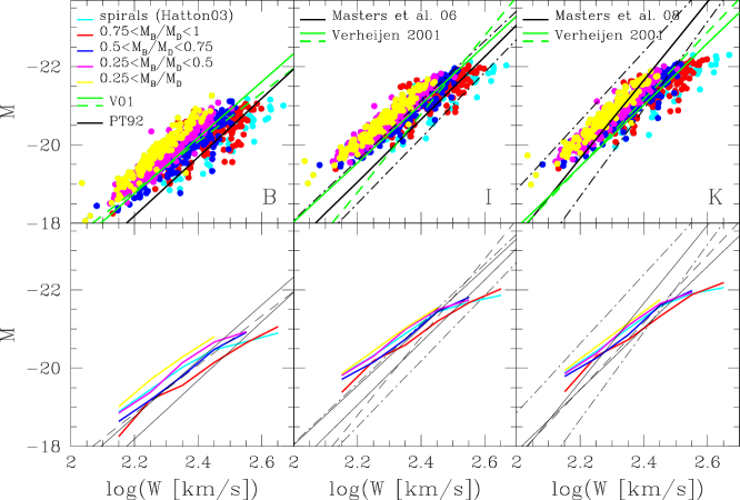
Figure 4: The $z=0$ Tully-Fisher relation in the B, I and K bands (from left to right). The upper panels show the scatter plots, while the lower panels show the median relations. In all panels, model spiral galaxies are selected according to $M_{\rm bulge}/M_{\rm disk}$ (see text). (Left panel): the B-band model TF (left panel) is compared with the observed relation by Verheijen (2001, green solid/dashed lines, see text) and Pierce & Tully (1992; solid black line). (Central panel): the I-band model TF is compared with the observed one from Masters et al. 2006 (black solid line for the relation, and dot-dashed lines for its scatter) and Verheijen 2001 (green solid/dashed lines). (Right panel): the K-band model TF relation is compared with the observed relation by Masters et al. (2008; solid black line for the relation, and dot-dashed lines for its scatter) and Verheijen 2001 (green solid/dashed lines).

Figure (4) shows the predicted $z=0$ Tully-Fisher relation in the B, I and K bands (from left to right); scatter plots are shown in the upper panels, while the median relations are shown in the lower panels. Disk galaxies in the model are selected according to the $M_{\rm bulge}/M_{\rm disk}$ criterium: yellow for $M_{\rm bulge}/M_{\rm disk}<0.25$, magenta for $0.25<M_{\rm bulge}/M_{\rm disk}<0.5$, blue for $0.5<M_{\rm bulge}/M_{\rm disk}<0.75$ and red for $0.75<M_{\rm bulge}/M_{\rm disk}<1$. The whole sample of spiral galaxies selected following Hatton et al. (2003) in terms of the relative luminosity of bulge and disk is represented by the cyan dots. The model velocities are taken at the fiducial value of $2.2\ R_{\rm D}$. In all bands, we compare the model predictions with the observational relation by Verheijen (2001), which is represented by two lines, indicating a different selection criterium for the observed galaxies. The green solid line) represents the complete sample with a measured HI global profile, while the green dashed line) represent the RC subsample. In the B band, we also plot the observational relation from Pierce & Tully (1992; thick solid black line). In the I and K bands, we compare the model TF with the observational relation by Masters et al. (2006, 2008, black solid line for the relation, and dot-dashed lines for its scatter). The I-band TF relation by Masters et al. (2006) is coincident with the relation found by Giovannelli et al. (1997).

For the B band, the plot shows that the model is successful in reproducing the observed TF slope, expecially for the later-type disk galaxies, and lies instead on the bright side in terms of the zero point. The offset with the Pierce & Tully relation is substantial, while it amounts to $\sim 0.2-0.4$ mags with respect to the Verheijen relation. Notice the discrepancy between different observational relations as well; in particular, the relation by Pierce & Tully (1992) is on the faint side of the others, and in fact led to a measured value of the Hubble parameter $H_{0}\sim 85$ km/s/Mpc, much larger than more recent results. For this reason, we consider the discrepancy between the model TF and this particular observational relation less significant.

In the I band, the model is able to reproduce the slope of the I-band TF relation very well, and is offset in the zero-point by $\sim 0.2-0.4$ mags. The model scatter is also comparable to the observed one. The performance of the model TF is worse here than the results of Croton et al. (2006) and de Lucia et al. (2004), who compare their models with the observed relation of Giovannelli et al. (1997). Both the Croton et al. (2006) and de Lucia et al. (2004) models differ from ours in the stellar population models adopted; by using BC03 instead of M05, the TF is shifted towards fainter magnitudes. Moreover, their oversimplification of the rotation velocity recipe shifts the TF towards slower values.

In the K band, the agreement of the model predictions with the data is better than in the other bands. Consistently, the K band is less affected by uncertainties such as dust reddening. Although the model relation is accomodated inside the data scatter, we nonetheless notice a discrepancy in the slope, which is more evident than in other bands. We can also identify a cut in velocity, around $log(W)\sim 2.3$, below which the model galaxies are too bright.

Table 1: $z=0$ model TF relations, power-law fits

[$M_{\rm bulge}/M_{\rm disk}$]	[0,0.25]	[0.25,0.5]	[0.5,0.75]	[0.75,1.]	all spirals
B band
slope $\Delta M/\Delta\rm{log}W$	-7.48	-7.12	-6.52	-5.20	-4.95
zero point at $\rm{log}W=2.4$	-20.76	-20.48	-20.15	-19.91	-20.18
I band
slope $\Delta M/\Delta\rm{log}W$	-7.51	-6.66	-6.43	-5.33	-5.37
zero point at $\rm{log}W=2.4$	-21.50	-21.33	-21.12	-20.94	-21.11
K band
slope $\Delta M/\Delta\rm{log}W$	-7.97	-7.02	-6.74	-5.72	-5.71
zero point at $\rm{log}W=2.4$	-21.68	-21.47	-21.26	-21.07	-21.26

Table (1) lists the slopes and zero-points at $\rm{log}W=2.4$ of the model TF relations shown in Fig. (4), obtained with power-law fits of the kind $M-5\rm{log}h=a+b\rm{log}W$, separated by morphological types. Interestingly, in all the bands considered the model shows a net differentiation between morphological types, with the more disk-dominated galaxies following a steeper relation with brighter zero-points in all bands, while bulge-dominated objects show a flatter slope. The morphology dependece of the K-band TF will be investigated in detail later on.

Notice the turn in the model TF slope at the high-mass end, for earlier types; this is the combined effect of AGN feedback and bulge formation. On the one hand, in the more massive objects the onset of AGN activity quenches star formation and thus reduces the galaxy luminosity per unit mass, moving the objects below the relation. On the other hand, while at the low-mass end the mechanism of bulge formation is preferentially secular evolution, which does not introduce a large scatter in the galaxy stellar populations, at the high-mass end bulges form primarily through mergers, which contribute to increase the scatter and raise the mass-to-light ratio. In addition, the larger bulge masses boost the bulge contribution to the rotation curve and increases the rotation velocity. These factors combined push the model galaxies below the relation at the high-mass end, and increase the scatter in the relation. This may also be the cause why the velocity range covered by GalICS spirals is not as wide as the data. The model in fact does not seem to produce late-type galaxies that are massive enough (contrary to both the De Lucia et al. 2004 and Croton et al. 2006 models). If GalICS overpredicts the abundance of large bulges at the high-mass end, then the number of massive spirals evolving into early-types increases, and these objects are lost from the spiral selection. This is mirrored in the progressively larger scatter and flattening of the slope for earlier-type model spirals.

Overall, although the model produces a reasonable TF slope, its performance is unsatisfactory in the B band, it is marginally acceptable in the I band, and it is better, but not perfect, in the K band. The interplay between dynamics and baryonic physics that shapes the TF relation is affected by many factors. We argue that we have good control over the dynamical model for the galaxy rotation curves and the stellar population models, both of which are physically sensible. Other degrees of freedom are introduced by the supernovae feedback recipe, the chemical evolution model, the star formation history of the model galaxies, dust extiction, and the modeling of the data to obtain rest-frame quantities (although such adjustments as the $k$-correction are small for local samples). The increasingly good match between model and data from the optical to the near-infrared suggests two possible causes for the offset.

The first possible explanation is the treatment of dust reddening. The observed relations used for the comparison have been corrected for internal extinction. Verheijen (2001) argues that this correction amounts to up to 1.4 mags in the B band. Fluctuations in the dust corrections can be of the same order of the offset we see between model and data. The better agreement between model and data in the K band is therefore particularly significant in this scenario, since this band is basically unaffected by dust reddening (and in addition the $k$-correction performed on the data to obtained rest-frame magnitudes is relatively small). However, if internal extinction corrections were the main cause of the disagreement in the optical TF, this would imply that in all the observed relations the dust reddening has been sistematically underestimated, which seems implausible.

The disagreement between model and data is present in all bands, but it is much worse in the optical/blue bands, and presents a morphology dependence. This suggests that the cause may be found in the balance between the emissions of stellar populations of different ages, which means that the star formation histories in the model galaxies are not realistic. An excess of luminosity like the one we obtain, with a variance from B to K, may hint to an excessively slow decline of the star formation rate towards low redshifts. As will be shown later on, another hint in favour of this argument is the redshift evolution of the TF, the fact that the match between model and data gets better at higher redshifts.

4.2 Morphology dependence of the Tully-Fisher at z=0

From the previous Section it is evident that the ratio $M_{\rm bulge}/M_{\rm disk}$ plays a role in determining the slope of the model TF. In particular, as the bulge mass increases with respect to the disk, the slope of the model TF decreases and the scatter increases. In general, model late-types agree better with the observed slope. This is encouraging, as the samples of galaxies selected to observe the TF relation are usually biased towards late-type spirals, which tend to feature cleaner rotation curves, due to stronger emission lines (Masters et al., 2008)

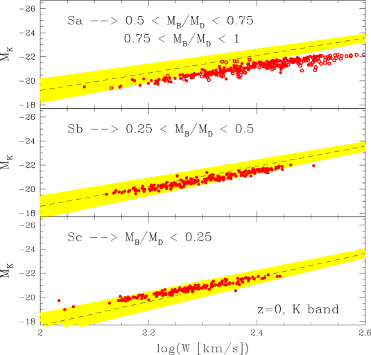
Figure 5: The morphology dependence of the $z=0$ K-band Tully-Fisher relation. The model predictions are compared with with data from Masters et al. (2008) (dashed solid lines, yellow shaded area representing the data scatter). From upper to lower: observed Sa galaxies compared with model galaxies with $0.5<M_{\rm bulge}/M_{\rm disk}<0.75$ (red dots) and galaxies with $0.75<M_{\rm bulge}/M_{\rm disk}<1$ (red circles); observed Sb galaxies compared with model galaxies with $0.25<M_{\rm bulge}/M_{\rm disk}<0.5$ (red dots); observed Sc galaxies compared with models galaxies with $0.25<M_{\rm bulge}/M_{\rm disk}$ (red dots).

The $M_{\rm bulge}/M_{\rm disk}$ ratio is a reasonable proxy for Hubble type, in that it gives a fair representation of the percentage of galaxy mass that is involved in star formation activity (model bulges do not receive cooling of fresh gas). Fig. (5) shows the morphology dependence of the $z=0$ model Tully-Fisher relation in the K band, according to our bulge/disk stellar mass classification. The results are shown in comparison with data from Masters et al. (2008; dashed black lines and yellow shaded area representing the relation and its scatter), and are divided according to Hubble type. In the upper panel, we compare observed Sa galaxies with the model galaxies with $0.5<M_{\rm bulge}/M_{\rm disk}<0.75$ (red dots), and we also show model galaxies with $0.75<M_{\rm bulge}/M_{\rm disk}<1$ (red circles); in the middle panel, we compare Sb types with model galaxies with $0.25<M_{\rm bulge}/M_{\rm disk}<0.5$ (red dots); in the lower panel we compare Sc types with model galaxies with $0.25<M_{\rm bulge}/M_{\rm disk}$ (red dots).

The model TF shows a differentiation with galaxy morphology, contributed by the more sophisticated recipe for the model rotation curves. The same differentiation is shown by the data, with later-type spirals exhibiting a shallower slope. The model TF is consistent with the data, with a good match with Masters et al. (2008) for Sb/Sc spirals (see Table 1), for velocities $log(W)>2.2$, although the slope is slightly different and the scatter is smaller. The model relation for Sa spirals is on the faint side of the data, with a clear bending of the slope at the high-mass end, due to the increasing bulge/disk mass ratio in the model galaxies. The success of the model in producing a morphology dependence of the TF shows that the balance between bulge and disk emission in the K band is correctly accounted for thanks to the use of the M05 stellar populations. Moreover, it also shows that the balance between the bulge and disk dynamics is effectively represented by the new rotation curve recipe.

As evident from Fig. (5) and the Figures in the previous Section, the model TF relation shows a small scatter for late-type galaxies, and an increasingly large scatter as the $M_{\rm bulge}/M_{\rm disk}$ ratio increases. This mirrors the different mechanism for bulge formation in late and early type spirals. Small bulges are likely to be formed entirely through secular evolution, they do not alter the rotation curve in a significant way, and their stellar populations are coeval with the ones in the disk. Massive bulges are more likely to be formed via mergers, which introduces a large random factor both in the ratio $M_{\rm bulge}/M_{\rm disk}$ and in the relative ages and chemical composition between disk and bulge stellar populations. The presence of a large bulge manifests itself with a steepening or a bump in the central part of the rotation curve, which increases the rotational velocity at $2.2\ R_{\rm D}$ at a given magnitude. Moreover, the presence of a massive bulge tends to dim the galaxy emission per unit mass (with respect to a disk-dominated object of the same mass). In addition to increasingly massive bulges, the downward trend at the very high-mass end of the theoretical relation, for the earlier types, is due to the onset of AGN feedback, that quenches star formation, and makes galaxies less luminous per unit mass.

Although we plotted the Masters et al. (2008) relation as a straight line, from their paper it is evident that this trend is visible in the data as well, and is apparent for Sa and Sb types. The model seems to mirror this behaviour, although in the data, it is observed at about $log(W)\sim 2.6$, while GalICS produces it around $log(W)\sim 2.4-2.5$. It is evident that GalICS cannot cover the mass range of the data due in part to the simulation limits; very large spirals are extremely rare in nature, and they occur with 0 probability in the simulation. Moreover, for increasing masses the model galaxies are more likely to experience mergers, which produce larger bulges and increase the $M_{\rm bulge}/M_{\rm disk}$ ratio; galaxies therefore are transformed into earlier types and progressively disappear from the TF relation.

4.3 Relative contribution of dynamics and stellar population models

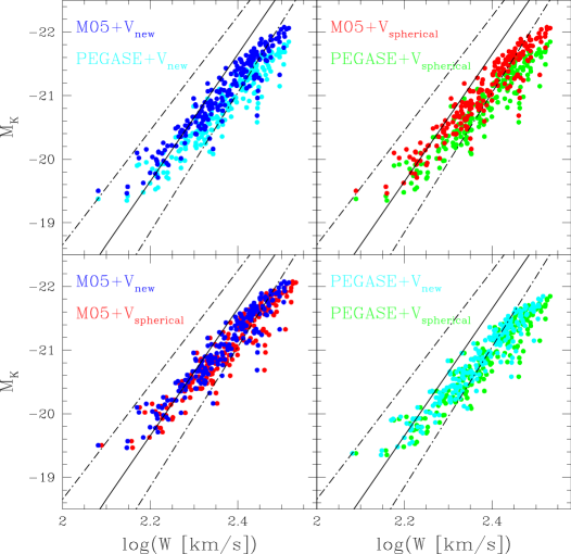
Figure 6: Relative contributions of the rotation curve recipe described in Section 2.1 and the stellar population models described in Section 2.2. In the four panels, the $z=0$ model TF relation in the K band is shown for the model Sa spirals, compared to the corresponding observed TF by Masters et al. (2008) (black solid line, see lower panel of Fig. (5)). In each panel, a different combination of dynamical model $-$ stellar population model is shown, between the ’new’ and ’spherical’ model for the rotation curve (see Section 2.1) and between M05 and PEGASE stellar population models (see Section 2.2), as indicated by the labels in each panel.

Fig. (6) summarizes the relative effects of a more precise and realistic model rotation curve, and of more complete stellar populations model. In the four panels, the $z=0$ model TF relation in the K band is shown for the Sa spirals (with errorbars representing its scatter), compared to the corresponding observed TF by Masters et al. (2008) (black solid line, see lower panel of Fig. (5)). In each panel, a different combination of dynamical model $-$ stellar population model is shown, between the ’new’ and ’spherical’ model for the rotation curve (see Section 2.1) and between M05 and PEGASE stellar population models (see Section 2.2). The effect of different rotation curve models and stellar population models on the TF is of comparable magnitude. The M05 run of the semi-analytic model produces a K-band TF brighter by $\sim 0.4$ mags than the PEGASE run. The ’new’ recipe for the rotation velocity shifts the TF by $\sim 20-30\%$ in velocity, depending on the galaxy mass and morphology. There is a certain degeneracy between the dynamics and stellar population models. The ’new’ dynamical model works better than the ’spherical’ for both stellar population models.

The analysis carried out so far implies that the model TF is flawed at $z=0$, in the B, I and K bands, even after we adopted refined and updated prescriptions for the galaxy rotation curves and the stellar populations. We use this conclusion to gain a better grasp of more profound problems of the model in reproducing the spiral population, in particular regarding the cooling and star formation histories at low redshifts, as will be discussed further in this work.

4.4 Satellites and the TF relation

Satellite galaxies in the simulation are defined as objects that do not reside in the center of the parent dark matter halo, but are orbiting around or infalling into a central galaxy. The gas in satellites is stripped because of ram pressure and tidal effects, while the cooling of new gas is prevented. This effectively shuts down star formation in satellite galaxies, which evolve passively unless a merger event takes place. For this reason, model satellite galaxies are ill-suited to be compared with real spirals. For the purpose of clarification and completeness, we show the predicted K-band TF relation for satellite spirals and compare them to centrals.

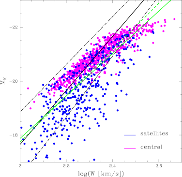
Figure 7: The predicted $z=0$ K-band Tully-Fisher relation, for a sample of model spirals in the range $0<M_{\rm bulge}/M_{\rm disk}<1$, and additionally split into central (magenta dots) and satellite (blue dots) galaxies. The model is compared with the observed relation by Masters et al. (2008; solid black line for the relation, and dot-dashed lines for its scatter) and Verheijen 2001 (green solid/dashed lines).

Fig. (7) shows the $z=0$ K-band TF relation for a sample of model spiral galaxies in the range $0<M_{\rm bulge}/M_{\rm disk}<1$, and additionally split into central (magenta dots) and satellite (blue dots) galaxies. It is clear that satellites do not follow a TF relation, but scatter below the central galaxy relation. The main reason is that satellites are less bright, due to the quenching of the star formation which, even if not affecting directly the K-band, raises the overall mass-to-light ratio. This affects expecially the low mass end of the satellite distribution.

Note that a significant fraction of the galaxies in the Master et al. samples are cluster galaxies, and they follow the same TF relation as the field samples. We can therefore use the TF relation as a tool to evaluate the ability of the model to reproduce the structure of satellite galaxies. We conclude without doubt that the model cannot produce realistic satellites. Again, the main problem resides in the star formation history. Real satellite spiral galaxies, although perturbed when in dense environments, are still star-forming, in particular those selected for TF studies. Hierarchical models, in order to reproduce the observed colour-magnitude relation, are forced to shut down star formation in satellites. This highlights a fundamental problem in hierarchical models, that certainly deserves further investigation.

5 Stellar mass vs K-band TF relation: S0 galaxies?

There is an ongoing debate about the formation of S0 galaxies. The origin of these objects is still not understood, but current scenarios include massive bulge formation, tidal stripping and star formation quenching as possible causes of a transition from spirals to S0, via a progressive fading of the disk (see Poggianti et al. 2001 and references therein). In particular, the possibility that S0 galaxies may be spiral galaxies where star formation has been shut down, and the spiral structure has thus become invisible, can be tested with the present study. An interesting consequence of this is the fact that the TF relation should present an offset between S0 and spiral galaxies (Williams et al. 2009, Bedregal et al. 2006, and references therein), which should be visible in the photometric TF but not in the stellar mass-velocity TF relation. However, Williams et al. (2009) find an offset between observed spirals and S0 both in the K-band TF and in the stellar TF, and therefore argue that S0 galaxies are not fading spirals. We use our model to verify whether star formation quenching introduces an offset between the stellar and K-band TF relation.

In this Section we show the model TF relation in the K-band, compared to the stellar TF relation $M_{\rm star}\ vs\ V_{\rm rot}$, for star-forming and nearly-passive disk galaxies at $z=0$. We again differentiate the galaxy morphology through the $M_{\rm bulge}/M_{\rm disk}$ ratio. Model disk galaxies with large $M_{\rm bulge}/M_{\rm disk}$ and low star formation rate should in principle present a spectral energy distribution similar to real S0 galaxies. First, the large bulges (built-up preferentially via minor mergers) and the small gaseous mass make these objects the transition point between spirals and ellipticals in the model. Second, the low star formation rates mimic the quenching due to gas stripping in dense environments as well as the natural fading due to the exhaustion of the gas reservoir.

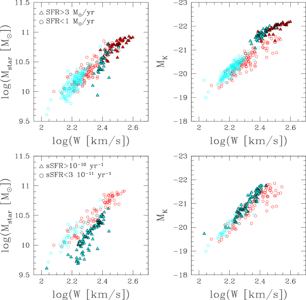
Figure 8: Comparison between the stellar and K-band TF relations for star-forming and non-star forming model galaxies. Left panels: model stellar TF relation at $z=0$. Right panels: model K-band TF relation at $z=0$. Upper panels: galaxies selected depending on their total star-formation rate. Triangles represent star forming galaxies with $SFR>3\ \rm M_{\odot}/yr$ and circles represent nearly-passive galaxies with $SFR<1\ \rm M_{\odot}/yr$. Lower panels: galaxies selected depending on ther specific star-formation rate. Triangles represent star forming galaxies with $sSFR>10^{-10}\ \rm yr^{-1}$ and circles represent nearly-passive galaxies with $sSFR<3\ 10^{-11}\ \rm yr^{-1}$. In all panels, galaxies are colour-coded according to morphology, with cyan circles/filled triangles representing ’later-types’ with $M_{\rm bulge}/M_{\rm disk}<0.5$, and red circles/filled triangles representing ’earlier-types’ with $0.5<M_{\rm bulge}/M_{\rm disk}<1$.

Fig. (8) shows the comparison between the $z=0$ stellar TF (left panels) and K-band TF (right panels) relations, for two subsamples of model galaxies divided according to the instantaneous SFR. In the upper panels, galaxies are selected depending on their total star-formation rate, and triangles show star-forming galaxies with $SFR>3\ \rm M_{\odot}/yr$, while circles represent nearly-passive galaxies with $SFR<1\ \rm M_{\odot}/yr$. In the lower panels instead, galaxies are selected according to their specific star formation rates, and triangles represent star-forming galaxies with $sSFR>10^{-10}\ \rm yr^{-1}$, while circles represent nearly-passive galaxies with $sSFR<3\ 10^{-11}\ \rm yr^{-1}$ (the separation between star-forming and nearly-passive was taken from Milky-Way values as a reference, see Munoz-Mateos et al., 2007). In all panels, galaxies are also colour-coded according to morphology, with cyan circles/filled triangles representing ’late-type’ spirals with $M_{\rm bulge}/M_{\rm disk}<0.5$, and red circles/filled triangles representing ’early-type’ spirals with $0.5<M_{\rm bulge}/M_{\rm disk}<1$. Red circles therefore represent the model rendition of S0-like objects (in terms of stellar populations).

When the galaxies are selected according to the total star-formation rate, we find a continuous stellar TF relation, as expected, between star-forming and nearly-passive galaxies, while we find a double sequence in the K-band, with the star-forming galaxies significantly brighter than their passive counterparts, for a given mass (the difference in mag is $\sim 0.5$, consistent with the findings of Williams et al.). We also find a morphology segregation in the K-band TF, with later-type spirals at the brigher end of the population (except the very top of the mass distribution, where later-types are not found in the model). This segregation tends to disappear in the stellar TF. This result seems to confirm that, indeed, S0 can be considered quiescent disks that are in the process of shutting down the star formation, and in this case the model S0 are represented by the red circles.

If we select the galaxies according to the specific star-formation rate, we find again a different trend between the stellar and K-band TF relations. The stellar TF relation shows a net segregation between star-forming and nearly-passive galaxies, which form a separate sequence. In addition, there is a net morphology segregation, which puts the earlier-types, nearly-passive galaxies at the massive end of the relation for any given velocity. In the K-band relation the star-forming, later-type galaxies are clearly on the brighter, lower-mass end of the relation for any given velocity. If we consider that the red circles as the model S0 galaxies, the picture is consistent with S0 galaxies being fading spirals. Earlier types, characterized by massive bulge formation, occupy the high-mass end of the population. The presence of a massive bulge reduces the fraction of galaxy mass that is actively star-forming, so that the specific star-formation rate and the luminosity are low compared with later-types of similar mass.

Although more investigation is needed on this topic, we are encouraged to conclude that the scenario that describes S0 galaxies are fading spirals is promising. We note that a direct comparison between our results and the findings of Williams et al. (2009) is problematic, due to the differences between the modeling of the dynamical mass by Williams et al. and the mass-velocity relation in GalICS. Further investigations on these results are under development

6 The redshift evolution of the TF up to z=1

The evolution of the TF is a good test of the galaxy assembly mechanism in the semi-analytic model, and here we present it in the optical and near-IR.

6.1 Evolution of the optical TF

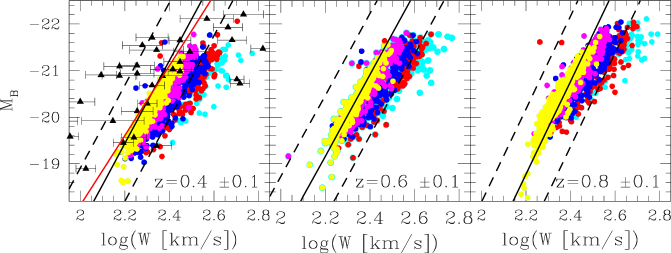
Figure 9: The redshift evolution of the rest-frame B-band Tully-Fisher relation from $z\sim 0.4$ to $z\sim 0.8$, compared with data from Fernandez-Lorenzo et al. (2009). Solid/dashed black lines represent the observed relation and its $2\sigma$ uncertainty, in all panels. In the $z=0.4$ panel, the data from Böhm & Ziegler (2007) are shown as black triangles. The relation by Bamford et al. (2006) at $<z>=0.33$ is also shown (red line). The model galaxies are represented by dots, colour-coded as in the previous Figures.

Fig. (9) shows the redshift evolution of the model rest-frame B-band TF relation from $z\sim 0.4$ to $z\sim 0.8$, compared with data from Fernandez-Lorenzo et al. (2009; black solid/dashed lines representing the observed relation and its scatter, in all panels), who derive the galaxy rotational velocity in a somewhat different manner than the rest of the published observational relations, based on optical line widths (see also Verheijen 2001 for a comparison between TF relations obtained with different velocity estimators). In the $z=0.4$ panel, data from Böhm & Ziegler (2007) are shown as black triangles, and the relation by Bamford et al. (2006) at $<z>=0.33$ is also shown for comparison. The colour-coding of the model dots is as in the previous Figures.

This figure shows a very good agreement between the model late-type spirals ($M_{\rm bulge}/M_{\rm disk}<0.5$, yellow and magenta points) and the data at $z\sim 0.6$ and $z\sim 0.8$, in slope, zero point and scatter. At $z\sim 0.4$ the model reproduces the observed slope, but tends to be slighly fainter in zero point (although still inside the observed $2\sigma$ uncertainty). Again, the model galaxies show a very clear morphological differentiation, and the earlier-types fall off the relation at the high-mass end at all redshifts, which as already discussed, is an effect mainly due to bulge formation, and AGN feedback.

The decline of the global SFR with time, together with the migration of the star formation to lower and lower galaxy masses (the downsizing effect), causes the galaxies to become fainter and the slope of the TF to get shallower at lower redshifts (also confirmed by the results of Weiner et al. 2006).

The model optical TF agrees very well with the data at high redshift, and by $z\sim 0.4$ the match starts to fail, where the model galaxies are too faint. By $z\sim 0$, the model is instead too bright (Fig. (4). This seems to confirm our suspicion that the model galaxy star formation histories are the main drivers of the discrepancy (or match) between model and data. At $z>0.5$ the model spiral galaxies seem to be quite realistic, while for lower redshifts the gas cooling, the accretion of substructures and the supernovae feedback conspire to produce an excessive star formation at odds with observations.

6.2 Evolution of the near-IR TF relation

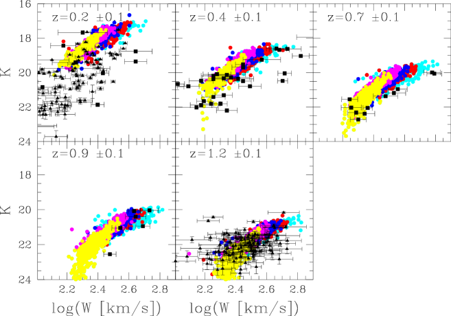
Figure 10: The redshift evolution of the observed-frame K-band Tully-Fisher relation from $z\sim 0.2$ to $z\sim 1.2$, compared with data from Fernandez-Lorenzo et al. (2010; solid black triangles) and Böhm & Ziegler (2007; solid black squares). The model galaxies are represented by dots, colour-coded as in the previous Figures.

Fig. (10) shows the evolution of the observed-frame K-band TF relation, in the redshift range from $z\sim 0.2$ to $z\sim 1.2$. The colour-coding of the model galaxies is the same as in the previous Figures. We compare the model predictions with data from Fernandez-Lorenzo et al. (2010; solid black triangles) and Böhm & Ziegler (2007; solid black squares). In this case the observed magnitudes are not corrected for dust extinction, so the model galaxy spectra are reddened according to their star-formation rate, as discussed in Section 2.

The scatter in the data here is large, and we do not attempt to determine the observed slopes and zero points. Nonetheless, the accord between the model TF and the observations is good in the range $0.4\leq z\leq 1.2$. Both the observed velocity range and luminosity range are well reproduced. The model galaxies also occupy the same velocity-luminosity space as the data. Moreover, the redshift evolution is reasonably well reproduced.

At $z\sim 0.2$, the model galaxies are too bright at the low-mass end, consistently with the results at $z=0$ (Fig. 4). Following the combined information of the evolution of the TF in the optical and near-IR, we argue that the model star formation histories are realistic down to $z>0.4$, and odd for lower redshifts.

7 Discussion

Disentangling the contributions of the different physical processes conspiring to produce the Tully-Fisher is not a trivial task. The slope and zero-point of the relation are determined by the interplay of the dynamics of galaxy assembly inside the dark matter halo, the cooling that regulates the gaseous and stellar content in each halo, the mass accretion and star formation histories and the supernovae feedback, all of which affect the structure and stability of disks as well as the evolution of the luminosity across all bands. Thus, matching the observed TF scaling relation is a fundamental check that the model is correctly predicting the formation and evolution of spirals.

However, a meaningful comparison with the observed TF necessitates of some fundamental steps, that ensure that there are no systematics that can offset the results. The first step is the correct modeling of the galaxy rotation curves, which are not directly predicted by the semi-analytic model itself, but need to be determined based on the galaxy fundamental dynamical quantities. The rotation curves extrapolate spatial information in model galaxies, following a dynamical recipe that is physically motivated and that needs to be as sophisticated as possible. In our ’new’ model, we made use of models for the mass distribution of the galactic components and angular momentum transfer to the disk accompanying bulge formation. It is worth noting that a complementary tool in this sense is represented by SPH simulations, which favour a detailed study of the galaxy structure, and are able to reproduce the TF relation for single galaxies, (e.g. Piontek & Steinmetz, 2009b), even if the shape of the rotation curve often remains unrealistic (see for instance Governato et al. 2007), and massive spiral galaxies still represent a problem. The sophistication of current SPH simulations also allows for detailed studies of the effects of perturbations such as ram-pressure on the rotation curves and the star formation (Kapferer et al. 2009, Kronenberg et al. 2008). However, the current resolution limits for this kind of simulations does not allow for cosmological runs and a statistical study.

The second step is the implementation of comprehensive stellar population models, which assures that the photometric side of the scaling relation is not marred by systematic offsets. We showed that this element can introduce a bias as large as 1 mag in the K-band, and 0.3-0.4 mag in the I band.

The third step is a consistency check in the comparison with observations, that presents challenges not related to the semi-analytic model itself. For instance, in a given band, observed TF relations sometimes are not consistent with one another, and the reason for these discrepancies is probably to be found in the data analysis. In fact, a significant degree of modeling of the raw data is required to produce an observed TF. To name a few, corrections are required for completeness, internal extinction, inclination, average distance and size in case of clusters, morphology, peculiar velocities (see for instance Masters et al. 2006). In addition, observed-frame magnitudes have to be converted into rest-frame through $k$-correction. and this introduces a further bias in the comparison. As we pointed out in Tonini et al. (2010), it is preferable to translate the semi-analytic model into observed-frame and compare the predictions with the apparent magnitudes. This is crucial expecially for star-forming objects, because their evolution is fast and the corrections are significant, (expecially for internal extinction and $k$-correction).

After the systematics in the modeling and in the comparison with data are taken care of in ’post-production’, the hierarchical model can be truly tested, and the problems of the model in reproducing the TF relation can be investigated.

7.1 Star-formation histories

The offset between the model and the observed TF relation has the following features: i) it depends on redshift, with a better agreement between model and data at higher redshift; ii) at redshift $z=0$ it depends on the photometric band, with a better agreement in the K band and the worst performance of the model in the B band; iii) it presents a morphology dependence across all redshifts and photometric bands. These facts suggest that the star formation history of the model galaxies is unrealistic, after $z\sim 0.4$. As a consequence, the predicted aging of the stellar populations is off, and the emission of stellar populations of different ages is unbalanced. In particular, the decline of star formation with time seems not to be fast enough, with the consequence that the fraction of the total stellar mass constituted of young and intermediate-age stellar populations is too high, a fact that predominantly affects the UV and optical bands, and the near-IR via the TP-AGB light. Note that this does not imply a wrong instantaneous SFR at $z=0$, which in fact is predicted to be consistent with observations (Hatton et al. 2003).

Central galaxies in a hierarchical model never stop accreting material, including fresh gas and gas previously expelled from the galaxy itself. Although this type of star formation history can be chaotic, in most cases at low redshifts GalICS star formation histories show a sufficiently steady decline to be approximated in the form of $\tau-$models: $SFR(t)=SFR_{0}exp(-t/t_{0})$. We calculated the predicted luminosity of model galaxies with different star formation timescales, and found the latter to be a fundamental parameter regulating the relative luminosities in B and K. For instance, a galaxy of age of $10\ \rm Gyr$ with a star-formation history like $SFR(t)=SFR_{0}exp(-t/10)$ (with a e-folding time $\tau=10\ \rm Gyr$) produces a B-band magnitude brighter by $\sim 0.83$ mags compared to a model like $SFR(t)=SFR_{0}exp(-t/3)$ (with a e-folding time $\tau=3\ \rm Gyr$), while it is brighter in the K-band by $\sim 0.46$ mags. From Fig. 4 it is evident that a shift of $\sim 0.83$ mags in the B band would produce a much better agreement between model and data, while at the same time, a shift of $\sim 0.46$ mags in the K band would still preserve the accord with the observed relations.

A faster decline of the star formation in time allows the galaxies to fade more rapidly at low redshifts, and brings the predicted TF relation down in luminosity. To size this effect, consider what happens to satellites after the star formation is shut down (Fig. 7). Also, as shown in all previous Figures, as more and more of the fraction of galaxy mass is in the inactive bulge component, or AGN feedback kicks in, the galaxy tends to fade and fall below the TF relation.

We argue that, in order to fix this problem, a more radical revision of gas infall and cooling is probably needed. A more detailed investigation of this point is of great interest, but it is beyond the present scope, in that it requires an extended comparison with SFR derived from observations at different redshifts. Note that the derivation of SFR from observations is affected by the adopted stellar population models, dust extinction corrections, star-formation history laws, as discussed in Maraston et al. (2010), and the use of inhomogeneous sets of such priors in comparison with our model will lead to significant biases. This line of investigation is currently under development

In addition to the star formation history, a second-order effect on the optical TF is caused by the chemical evolution model in use. The current version of GalICS implements the Pipino et al. (2009) recipe which, compared to Hatton et al. (2003), produces slightly lower total metallicities, causing the galaxies to be brighter. Depending on age and star formation history, the difference in magnitude amounts to anything between $0$ and $\sim 0.5$ in the B band, and less for the I and K bands. Accounting for uncertainties in the chemical evolution recipe would only lead to a modest increase of the TF scatter, which would be consistent with the scatter in the data, but it would not shift the overall relation in a significant way.

7.2 Disk scale-lenghts and the disk-halo connection

There is also the possibility that part of the discrepancies that we encountered in our comparison with data are due to a flaw in the modeling of the galactic dynamics. In particular, the galaxy rotation may be offset, regardless of the galaxy type, due to a wrong determination of the galaxy angular momentum. This can be investigate by analyzing the disk scale-lenghts $R_{\rm D}$ produced by the model.

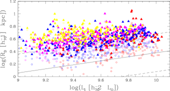
Figure 11: Model disk scale-lenghts as a function of I-band luminosity, compared with the relation obtained by Courteau et al. (2007) from observations (solid/dashed lines for the relation and its scatter). The empty dots represent model galaxies in the ’spheroidal’ model, colour-coded according to $M_{\rm bulge}/M_{\rm disk}$ as in the previous Figures. Filled triangles represent the same galaxies after angular momentum transfer from the bulge is evaluated (the ’new’ model).

Figure 11 shows the model disk scale-lenghts as a function of I-band luminosity, compared with the relation obtained by Courteau et al. (2007) from observations (solid/dashed lines for the relation and its scatter). The empty dots represent model galaxies in the ’spheroidal’ model, colour-coded according to $M_{\rm bulge}/M_{\rm disk}$ as in the previous Figures. Filled triangles represent the same galaxies after angular momentum transfer from the bulge is evaluated (the ’new’ model).

It is evident that the model cannot reproduce the Courteau et al. relation. The disk-scale lenght appears to be too large, and the scatter too big, the latter a problem that was mentioned already in Hatton et al. (2003). More in detail, the model does not reproduce the Courteau et al. relation for the late-type spirals (yellow points), which are mostly untouched by our ’new’ velocity model. In the old ’spheroidal’ model, the earlier-type spirals present a marginal agreement with the data, which we argue is accidental. In fact, the values of the disk-scale lenghts inferred from observations are commonly obtained by fitting the surface brightness profile with an exponential law, and that the result is more accurate the closer the galaxy is to a pure disk. Galaxies with large bulges are not ideal candidates, and they tend to be excluded from the observational samples. The ’new’ model effectively corrects for the presence of the bulge, moving the earlier-type spirals in the same $R_{\rm D}-L_{\rm I}$ space as the later-types, in a sense making all galaxies consistently offset with the Courteau et al. relation.

Before analyzing the possible causes of the discrepancy, it should be noted that a source of error stems from the use of Eq. (3) for the determination of $R_{D}$. This formula, adopted by Hatton et al. 2003, produces the highest $R_{D}$ under angular momentum conservation, in the MMW formalism. Additional shape factors that can reduce the value of $R_{D}$ are set to unity, but as discussed in Tonini et al. (2006a), their values as inferred from observed rotation curves are actually close to unity, and vary slowly with disk mass.

As for the cause of the discrepancy with the Courteau data, we offer 2 explanations:

I) as discussed in Tonini et al. (2006a) and D’Onghia & Burkert (2004), the halo spin parameter, which is found to vary from $<\lambda>=0.04$ in GalICS to $<\lambda>=0.05$ in other simulations, is too high compared with the one that can be inferred from observations of spirals. If $<\lambda>=0.03$ for instance (the value inferred by Tonini et al. 2006a), then Rd is smaller by $\sim 25\%$, which would push our model $R_{\rm D}$ towards the Courteau et al. relation. Note that, although $\lambda$ originates naturally from tidal forces during structure formation, the discrepancy between the simulated and observed $\lambda$ is not necessarily due to a flaw in the simulations, but rather it hints at a subsequent redistribution of angular momentum between baryons and dark matter;

II) as mentioned in Section (2.1), the ratio $j_{\rm D}/m_{\rm D}$ is equal to unity only under angular momentum conservation, which is not a realistic scenario during galaxy formation. In particular, if the baryonic component that collapses to form the protogalaxy is clumpy, it likely dissipates angular momentum in its path to the centre of the dark matter halo, as proposed by Tonini et al. (2006b), and therefore $j_{\rm D}/m_{\rm D}<1$. Consequently, the disk scale-length is smaller, and the tension between model $R_{D}$ and observations is partially alleviated ($j_{\rm D}/m_{\rm D}\sim 0.75$ leads to a decrease of $R_{\rm D}$ by $\sim 25\%$). The MMW recipe can therefore be considered a ’maximal scale-length scenario’, with the real scale-length distribution being centered on smaller values of $R_{D}$ because of angular momentum transfer.

Both the effects described above contribute in reducing the size of $R_{D}$, and are currently not investigated in semi-analytic models. Note also that such effects do not depend on redshift nor on photometric band, therefore they do not affect our conclusions on the model star formation histories discussed in the previous section.

An additional, largely unknown source of scatter, on both the disk scale-lengths and the rotation curve, is represented by the dark matter halo structural evolution. On the one side, readjustments in the halo profile induced by the baryon infall can lead to a dramatic change in the inner density profile (Tonini et al. 2006b), thus altering the contribution of the halo to the total velocity. On the other side, tidal interactions between halos and mass accretion in the hierarchical assembly repeatedly strip and add material in each halo. There is no standard recipe in semi-analytic models to recalculate the halo equilibrium structure that takes into account all these effects, and since there is no spatial information inside single objects, the mass is the primary driver of halo evolution. The virial radius in particular is not recalculated after every interaction, with the consequence that the halo density profile can oscillate quite a lot. Note that also in N-body simulations, although all halos are fitted to a common functional profile (like the NFW or the isothermal sphere), the scatter on the profile is very large, as is the scatter on the mass-virial radius relation (Bullock et al. 2001). The scatter in the virial radius directly translates into a scatter in $R_{D}$, while the scatter in the density profile affects the halo velocity. In particular, an overestimation of the disk scale-lengths will occurr in cases where the mass loss via tidal stripping dominates the halo evolution.

The offset between model and observed disk scale-lengths represents an interesting failure of the model, that arguably sheds light on some missing physics. These considerations suggest that baryon cooling and halo structural evolution in the model need some more fundamental revision, which is beyond the scope of the present work.

8 Summary and conclusions

We analyzed the predictions of the hierarchical galaxy formation model GalICS on the Tully-Fisher relation and its evolution with redshift. We introduced two new elements in the model: 1) a new recipe for the determination of the galaxy rotation curves, based on the correct dynamical modeling of the different galactic components, and taking into account the angular momentum exchange between bulge and disk due to secular evolution; 2) the M05 stellar population models, that include an exhaustive treatment of the TP-AGB emission, which affects galaxies with ongoing star formation.

Our main conclusions are:

$\bullet$ the improvement on the dynamical description of disk galaxies and on the stellar population models impacts the model TF by effects of comparable magnitude; in particular, velocities are shifted to values lower by $\sim 0-50\%$ depending on the galaxy mass and morphology, and the K-band magnitudes are brighter by $\sim 0.2$ mags at redshift zero and up to $>1$ mags at redshift $z\sim 1$ and above;

$\bullet$ at redshift $z=0$ the model reproduces the slope of the observed TF for Sb/Sc spirals, in the B, I and K band, but not the zero-point, which is too bright in all bands. In particular, in the K band the zero-point is too bright for Sb/Sc galaxies at the low-mass end ($log(W)<2.3$), although the model galaxies lie within the scatter of the observed TF relation. In the B and I band, the predicted zero-point for Sb/Sc galaxies is too bright across the mass range. We argue that the most probable cause of the discrepancy lies in unrealistic star-formation histories at $z<0.4$;

$\bullet$ the model predicts a morphology dependence of the TF relation at all redshifts. At $z=0$ observations in the K-band confirm this trend, and the comparison between model and data is encouragingly good, expecially for Sb/Sc spirals. This is an important confirmation that our more sophisticated treatment of the galaxy dynamics is realistic. The model rotation curve now mirrors the morphological differentiation observed in nature, well representing the balance between bulge and disk, and the consequent variations in the predicted TF along the Hubble sequence are put in sharper evidence. The model predicts a steeper slope and a smaller scatter for later-type galaxies, and a progressive flattening of the slope and larger scatter for earlier types. This is coherent with the picture of bulge formation in a hierarchical scenario, where the incidence of mergers is significant in the case of massive bulges, while small bulges are more likely to develop via secular evolution. Moreover, with the M05 stellar population models, GalICS is able to correctly reproduce the balance between the bulge and disk emission in the K band;

$\bullet$ the scatter in the model galaxies increases from late types (Sb/Sc) to early types (Sa/S0), because the main mechanism for bulge formation switches from secular evolution (Sb/Sc) to minor mergers (Sa/S0). At the high-mass end, earlier-type galaxies show a flattening of the slope and tend to fall below the relation due to the presence of massive bulges and AGN feedback;

$\bullet$ the study of the TF relation for model satellites galaxies confirms previous hints that the model cannot produce realistic non-central spirals;

$\bullet$ the TF relation can be used as a discriminating tool to investigate the origin of S0 galaxies, in the scenario where these objects form from the fading of spirals after star-formation shutdown;

$\bullet$ the model reproduces the redshift evolution of the TF for later-type galaxies from $z=0.8$ to $z=0.4$ in the rest-frame B band, where slope, zero-point and scatter are reproduced for Sb/Sc spirals. The model is consistent with the data in the observed-frame K band at redshifts between $z=1.2$ and $z=0.4$. The simultaneous match in the optical and near-IR evolution, although needing more tests with larger data samples, indicates that the mass assembly and star formation histories, as well as the supernovae feedback implementation, are satisfactory at these redshifts;

$\bullet$ the model cannot reproduce the whole optical Tully-Fisher evolution from $z\sim 0$ to $z\sim 1.2$. We argue that the decline of the star formation is too slow, thus preventing the model from matching simultaneously the local and distant relations;

$\bullet$ the model produces disk scale-lengths too large compared with observations. We argue that this mirrors a too simplistic recipe of disk formation inside dark matter halos, that does not take into account angular momentum redistribution during the baryonic collapse.

References

- Balland (2003) Balland, C., Devriendt, J. E. G. & Silk, J., 2003, MNRAS, 343, 107
- bamford (2006) Bamford, S. P., Aragón-Salamanca, A. & Milvang-Jensen, B., 2006, MNRAS, 366, 308B
- barmby (2008) Barmby, P., et al., 2008, ApJS, 177, 431
- baugh (1996) Baugh, C.M., Cole, S. & Frenk, C.S., 1996, MNRAS, 283, 1361B
- baugh (2005) Baugh, C. M., Lacey, C. G., Frenk, C. S., Granato, G. L., Silva, L., Bressan, A., Benson, A. J. & Cole, S., 2005, MNRAS, 356, 1191B
- bedregal (2006) Bedregal, A. G., Aragon-Salamanca, A. & Merrifield, M. R., 2006, MNRAS, 373, 1125
- benson (2003) Benson, A. J., Bower, R. G., Frenk, C. S., Lacey, C. G., Baugh, C. M. & Cole, S., 2003, ApJ, 599, 38
- benson (2010) Benson, A.J. & Bower, R. G., 2010, MNRAS, 405, 1573
- bett (2007) Bett, P., Eke, V., Frenk, C. S., Jenkins, A., Helly, J. & Navarro, J., 2007, MNRAS, 376, 215
- binney (2008) Binney, J. & Tremaine, S., 2008, ’Galactic dynamics’, Princeton University Press
- blanton (2007) Blanton, M.R. & Roweis, S., 2007, AJ, 133, 734
- blumenthal (1986) Blumenthal, G.R., Faber, S.M., Flores, R. & Primack, J.R., 1986ApJ, 301, 27B
- bohm (2004) Böhm, A., et al., 2004, A&A, 420, 97
- bohm (2004) Böhm, A. & Ziegler, B.L. 2007, ApJ, 668, 846
- Bower (2006) Bower, R.G., Benson, A.J., Malbon, R., Helly , J.C., Frenk, C.S., Baugh, C.M., Cole, S., & Lacey, C.G. 2006, MNRAS, 370, 645
- bullock (2001) Bullock, J. S., Dekel, A., Kolatt, T. S., Kravtsov, A. V., Klypin, A. A., Porciani, C. & Primack, J. R., 2001, ApJ, 555, 240
- bundy (2005) Bundy, K., Ellis, R.S. & Conselice, C.J., 2005, ApJ, 625, 621
- bundy2 (2006) Bundy, K., et al., 2006, ApJ, 651, 120B
- catinella (2005) Catinella, B., Haynes, M.P. & Giovanelli, R., 2005, AJ, 130, 1037
- cattaneo (2008) Cattaneo, A., Dekel, A., Faber, S.M. & Guiderdoni, B., 2008, MNRAS, 389, 567C
- coil (2004) Coil, A.L., et al., 2004, ApJ, 617, 765
- Cole (2000) Cole, S., Lacey, C.G., Baugh, C.M., & Frenk, C.S. 2000, MNRAS, 319, 168
- courteau (2007) Courteau, S., Dutton, A.A., van den Bosch, F.C., MacArthur, L.A., Dekel, A., McIntosh, D.H. & Dale, D.A., 2007, ApJ, 671, 203C
- Croton (2006) Croton, D. J., Springel, V., White, S. D. M., De Lucia, G., Frenk, C. S., Gao, L., Jenkins, A., Kauffmann, G., Navarro, J. F. & Yoshida, N., 2006, MNRAS, 365, 11
- dale (1998) Dale, D.A., 1998, Ph.D. thesis, Cornell Univ
- dale (1998) Dale, D.A., Giovanelli, R., Haynes, M.P., Hardy, E. & Campusano, L.E., 1999, AJ, 118, 1468
- davis (2003) Davis. M., et al., 2003, SPIE, 4834, 161D
- davis (2007) Davis. M., et al., 2007, ApJ, 660, L1
- debattista (2006) Debattista, V.P., Mayer, L., Carollo, C., Moore, B., Wadsley, J. & Quinn, T., 2006, ApJ, 645, 209
- DeLucia04 (2004) De Lucia, G., Kauffmann, G. & White, S. D. M., 2004, MNRAS, 349, 1101
- 2004 ([donghia) ’Onghia, E. & Burkert, A. M., 2004, ApJ, 612, L13
- duffy (2010) Duffy, A. R., Schaye, J., Kay, S. T., Dalla Vecchia, C., Battye, R. A. & Booth, C. M., 2010, MNRAS, 405, 2161
- dutton (2007) Dutton, A.A., van den Bosch, F.C., Dekel, A. & Courteau, S., 2007, ApJ, 654, 27D
- dutton (2007) Dutton, A.A. & van den Bosch, F.C., 2009, MNRAS, 396, 141
- fall (1980) Fall, S. M. & Efstathiou, G., 1980, MNRAS, 193, 189F
- fernandez (2009) Fernandez Lorenzo, M., Bongiovanni, A., Castaneda, H., Perez Garcia, A.M., Lara-Lopez, M.A., Povic, M. & Sanchez-Portal, M., 2009, A&A, 496, 389F
- fernandez (2010) Fernandez Lorenzo, M., Cepa, J., Bongiovanni, A., Perez Garcia, A.M., Lara-Lopez, M.A., Povic, M. & Sanchez-Portal, M., 2010, arXiv:1005.1512v1
- Fioc & Rocca-Volmerange (1997) Fioc, M., & Rocca-Volmerange, B. 1997, A&A 326, 950
- firmani (1999) Firmani, C. & Avila-Reese, V., 1999, ASPC, 176, 406
- giovanelli (1994) Giovanelli, R., Haynes, M.P., Salzer, J.J., Wegner, G., da Costa, L.N. & Freudling, W. 1994, AJ, 107, 2036Q
- giovanelli (1995) Giovanelli, R., Haynes, M.P., Salzer, J.J., Wegner, G., da Costa, L.N. & Freudling, W. 1995, AJ, 110, 1059
- giovanelli (1997) Giovanelli, R., Haynes, M., Herter, T., Vogt, N.P., Wegner, G., Salzer, J.J., da Costa, L.N. & Freudling, W. 1997a, AJ, 113, 22
- giovanelli (1997) Giovanelli, R., Haynes, M., Herter, T., Vogt, N.P., Wegner, G., Salzer, J.J., da Costa, L.N. & Freudling, W. 1997b, AJ, 113, 53
- governato (2007) Governato, F., William, B., Mayer, L., Brooks, A., Stinson, G., Valenzuela, O., Wadsley, J. & Quinn, T., 2007, MNRAS, 374, 1479
- graham (2008) Graham, A. W. & Worley, C. C., 2008, MNRAS, 388, 1708
- Hatton (2003) Hatton, S., Devriendt, J.E.G., Ninin, S., Bouchet, F.R., Guiderdoni B. & Vibert, D. 2003, MNRAS, 343, 75
- haynes (1999) Haynes, M.P., Giovanelli, R., Chamaraux, P., da Costa, L.N., Freudling, W., Salzer, J.J. & Wegner, G., 1999a, AJ, 117, 2039
- haynes (1999) Haynes, M.P., Giovanelli, R., Salzer, J.J.,Wegner, G., Freudling,W., da Costa, L.N., Herter, T. & Vogt, N.P., 1999b, AJ, 117, 1668
- heidt (2003) Heidt, J., et al., 2003, A&A, 398, 49
- henriques (2010) Henriques, B., Maraston, C., Monaco, P., Fontanot, F., Menci, N., De Lucia, G. & Tonini, C., 2010, in preparation
- hernquist (1990) Hernquist, L., 1990, ApJ, 356, 359H
- hetz (2006) Hetznecker, H. & Burkert, A., 2006, MNRAS, 370, 1905
- hohl (1971) Hohl, F., 1971, ApJ, 168, 343
- kauffmann (1993) Kauffmann, G., White, S. D. M., & Guiderdoni, B., 1993, MNRAS, 264, 201
- kapferer (2009) Kapferer, W., Sluka, C., Schindler, S., Ferrari, C. & Ziegler, B. L., 2009, A&A, 499, 87
- kronberger (2008) Kronberger, T., Kapferer, W., Unterguggenberger, S., Schindler, S. & Ziegler, B. L., 2008, A&A, 483, 783
- lin (2007) Lin, L., et al., 2007, ApJ, 660, L51
- maccio (2007) Maccio, A. V., Dutton, A. A., van den Bosch, F. C., Moore, B., Potter, D. & Stadel, J., 2007, MNRAS, 378, 55
- maller (2002) Maller, A. H. & Dekel, A., 2002, MNRAS 335, 487
- Maraston (2005) Maraston, C. 2005, MNRAS, 362, 799
- Maraston (2006) Maraston, C., Daddi, E., Renzini, A., Cimatti, A., Dickinson, M., Papovich, C., Pasquali, A. & Pirzkal, N. 2006, ApJ, 652, 85M
- Maraston (2010) Maraston, C., Pforr, J., Renzini, A., Daddi, E., Dickinson, M., Cimatti, A. & Tonini, C., 2010, MNRAS, 407, 830
- karen2 (2008) Masters, K.L., Springbob, C.M.. Haynes, M.P. & Giovanelli, R., 2006, ApJ, 653, 861M
- karen1 (2008) Masters, K.L., Springbob, C.M. & Huchra, J.P., 2008, AJ, 135, 1738M
- mcgaugh (2010) McGaugh, S. S., Schombert, J. M., de Blok, W. J. G. & Zagursky, M. J., 2010, ApJ, 708L, 14M
- Menci (2005) Menci, N., Fontana, A., Giallongio, E., Grazian, A., & Salimbeni, S. 2006, ApJ, 647, 753
- mo (1998) Mo, H.J., Mao, S. & White, S.D.M., 1998, MNRAS, 295, 319M
- Monaco (2007) Monaco, P., Fontanot, F., & Taffoni, G. 2007, MNRAS, 375, 1189
- Munoz-Mateos (2007) Munoz-Mateos, J. C., Gil de Paz, A., Boissier, S., Zamorano, J., Jarrett, T., Gallego, J. & Madore, B. F., 2007, ApJ, 658, 1006
- nfw (1997) Navarro, J. F., Frenk, C. S. & White, S. D. M., 1997, ApJ, 490, 493
- pierce (1992) Pierce, M.J. & Tully, R.B., 1992, ApJ, 387, 47
- piontek (2009) Piontek, F. & Steinmetz, M., 2009arXiv0909.4156P
- piontek2 (2009) Piontek, F. & Steinmetz, M., 2009arXiv0909.4167P (b)
- pipino (2009) Pipino, A., Devriendt, J.E.G., Thomas, D., Silk, J. & Kaviraj, S., 2009, A&A, 505, 1075P
- poggianti (2010) Poggianti, B. M., et al., 2001, ApJ, 563, 118P
- salucci (2007) Salucci, P., Lapi, A., Tonini, C., Gentile, G., Yegorova, I.A. & Klein, U., 2007, MNRAS, 378, 41S
- simien (1986) Simien, F. & de Vaucouleurs, G., 1986, ApJ, 302, 564S
- Somerville (2008) Somerville, R. S., Hopkins, P. F., Cox, T. J., Robertson, B. E., & Hernquist, L., 2008, MNRAS, 391, 481
- springbob (2005) Springbob, C.M., Haynes, M.H., Giovanelli, R. & Kent, B., 2005, ApJS, 160, 149
- Tonini (2006) Tonini, C. Lapi, A., Shankar, F. & Salucci, P., 2006, ApJ, L638, 13T
- Tonini (2006) Tonini, C., Lapi, A. & Salucci, P., 2006 ApJ, 649, 591T
- Tonini (2009) Tonini, C., Maraston, C., Devriendt, J., Thomas, D. & Silk, J. 2009, MNRAS, 396L, 36T
- Tonini (2010) Tonini, C., Maraston, C., Thomas, D., Devriendt, J. & Silk, J., 2010, MNRAS.tmp..209T (2009arXiv0910.0015T)
- trujillo (2010) Trujillo-Gomez, S., Klypin, A., Primack, J. & Romanowsky, A. J., 2010, arXiv:1005.1289v2
- tf (1977) Tully, R.B., & Fisher, J. R., 1977, A&A, 54, 661T
- tully (1985) Tully, R.B. & Fouqué, P. 1985, ApJS, 58, 67
- tully (1996) Tully, R.B., Verheijen, M.A.W., Pierce, M.J., Huang, J.-S. & Wainscoat, R.J. 1996, AJ, 112, 2471
- tully (1998) Tully, R.B., Pierce, M.J., Huang, J.-S., Saunders, W., Verheijen, M.A.W. & Witchalls, P.L., 1998, AJ, 115, 2264
- vdb00 (2000) van den Bosch, F. C., 2000, ApJ, 530, 177
- vdb02 (2002) van den Bosch, F. C., 2002, MNRAS, 332, 456
- vdb (2002) van den Bosch, F. C., Abel, T., Croft, R.A.C., Hernquist, L. & White, S.D.M., 2002, ApJ, 576, 21
- vanderWel (2006) van der Wel, A., Franx, M., Wuyts, S., van Dokku, P. G., Huang, J., Rix, H-W. & Illingworth, G. D., 2006, ApJ, 652, 97
- ver (2001) Verheijen, M.A.W., 2001, ApJ, 563, 694V
- vitvitska (2002) Vitvitska, M., Klypin, A. A., Kravtsov, A. V., Wechsler, R. H., Primack, J. R. & Bullock, James S., 2002, ApJ, 581, 799
- vogt (1995) Vogt, N.P., 1995, PhD thesis, Cornell Univ
- weiner (2006) Weiner, B. J., Willmer, C. N. A., Faber, S. M., Harker, J., Kassin, S. A., Phillips, A. C., Melbourne, J., Metevier, A. J., Vogt, N. P. & Koo, D. C., 2006, ApJ, 653, 1049W
- williams (2009) Williams, M. J., Bureau, M. & Cappellari, M., 2009, proceeding of the conference ”Hunting for the Dark: The Hidden Side of Galaxy Formation”, Malta, 19-23 Oct. 2009, eds. V.P. Debattista & C.C. Popescu, AIP Conf. Ser., in press; arXiv:0912.5088v1
- irina (2007) Yegorova, I.A. & Salucci, P., 2007, MNRAS, 377, 507Y