Solar abundance corrections
derived through 3D magnetoconvection simulations

Abstract

We explore the effect of the magnetic field when using realistic three-dimensional convection experiments to determine solar element abundances. By carrying out magnetoconvection simulations with a radiation-hydro code (the Copenhagen stagger code) and through a-posteriori spectral synthesis of three Fe i lines, we obtain evidence that moderate amounts of mean magnetic flux cause a noticeable change in the derived equivalent widths compared with those for a non-magnetic case. The corresponding Fe abundance correction for a mean flux density of $200$ G reaches up to $\sim 0.1$ dex. These results are based on space- and time-averaged line profiles over a time span of $2.5$ solar hours in the statistically stationary regime of the convection. The main factors causing the change in equivalent widths, namely the Zeeman broadening and the modification of the temperature stratification, act in different amounts and, for the iron lines considered here, in opposite directions; yet, the resulting $|\Delta\log\epsilon_{\odot}(Fe)|$ coincides within a factor two in all of them, even though the sign of the total abundance correction is different for the visible and infrared lines. We conclude that magnetic effects should be taken into account when discussing precise values of the solar and stellar abundances and that an extended study is warranted.

1 Introduction

The advent of increasingly realistic three-dimensional convection simulations based on radiation-hydrodynamics codes (Dravins et al., 1981; Nordlund, 1985; Freytag et al., 2002; Vögler et al., 2005) has led to the conclusion that horizontal inhomogeneities and departures from Local Thermodynamic Equilibrium (LTE) are crucial for an accurate abundance determination (see the review by Asplund, 2005). Three-dimensional hydrodynamic (HD) models have allowed to remove many uncertainties in abundance determination, in particular those coming from the use of micro- and macroturbulence velocity parameters (Asplund et al., 2000a). Yet, several sources of uncertainty remain, resulting, e.g., from possible blending of lines, errors in continuum measurements, equivalent width determination (Holweger, Kock, & Bard, 1995; Blackwell, Smith, & Lynas-Gray, 1995; Kostik, Shchukina & Rutten, 1996; Ayres, 2008a, b; Caffau et al., 2008) or calculation of collisions with H atoms (Fabbian et al., 2006, 2009). Another potentially important source of uncertainty stems from the presence of significant amounts of magnetic flux in the photosphere of the quiet Sun (Stenflo, 1982; Sánchez Almeida, Emonet & Cattaneo, 2003; Shchukina & Trujillo Bueno, 2003; Trujillo Bueno, Shchukina & Asensio Ramos, 2004) and its possible influence on the average width of the line profiles (Stenflo & Lindegren, 1977). The purpose of this Letter is to use 3D magnetoconvection (MHD) models to estimate the influence of the magnetic field on the spectral profiles of a number of Fe i lines, and to translate the difference between the equivalent widths in MHD and HD models to the corresponding Fe abundance corrections.

The impact of magnetic fields on chemical abundance determinations has so far been widely neglected. It was implicitly assumed that the magnetic field should not play a major role in changing the shapes of spatially-averaged spectral lines, as these averages are weighted towards granules (Nordlund, Stein, & Asplund, 2009), while magnetic concentrations are thought to reside mainly in intergranular lanes (Khomenko et al., 2003). Still, Borrero (2008) found that the neglect of magnetic broadening can lead to a systematic error of up to $0.1$ dex in the abundance determination of iron. The author used 1D spectral synthesis with uniform magnetic field in a plane-parallel atmosphere, therefore inevitably neglecting the effect of the field on the temperature stratification. However, the latter effect, although indirect, can be important (see, e.g. Socas-Navarro & Norton, 2007) and must be considered alongside the direct effect through Zeeman broadening (see, e.g. Stenflo & Lindegren, 1977).

Iron is one of the crucial chemical elements for a variety of reasons like: (a) it is widely used to define a metallicity scale, hence as a proxy for the overall metal content; (b) the effect of the magnetic field on the line profiles seem to be more pronounced for this element than for, e.g. Si, C and O (Borrero, 2008); (c) the large amount of iron lines in the solar spectrum allows to consider features with high Landé factor. It is therefore advisable to start with iron when studying the magnetic effects on abundance determinations from MHD models. In this Letter, we present results based on a series of three-dimensional magneto-convection simulations. Our aim is to explore, understand and constrain the possible impact on the solar abundance determination of self-consistent, simultaneous 3D and magnetic effects. These effects are studied via comparison of the equivalent widths for the magnetic cases with those obtained in HD conditions. To derive the necessary abundance correction, we match the MHD equivalent width with that obtained on the basis of HD runs with changed abundance. Our analysis focuses on quiet Sun conditions. We conclude that magnetic effects, in particular via modification of the average temperature stratification, should be taken into account when considering the solar abundance problem.

2 Simulations and spectral synthesis

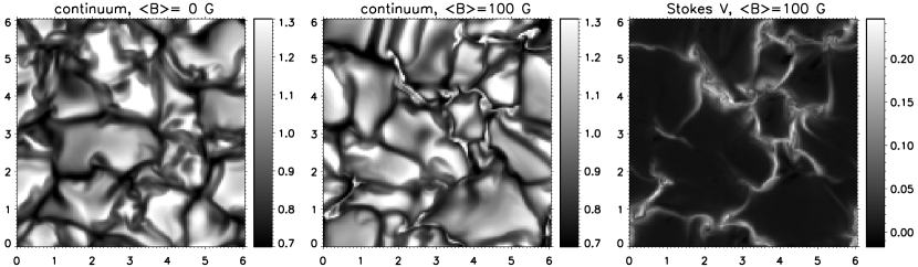
Figure 1: Emerging continuum intensity at 608 nm in the HD simulation run (left), and in the MHD run with “100 G” setup (center). Note the appearance of intergranular bright points after introducing magnetic flux. The right panel shows the amplitude of Stokes V, defined as max($|\textrm{V}|$) in units of the continuum intensity, sign included.

The results in this paper are based on simulations we carried out using the Copenhagen stagger-code (Nordlund & Galsgaard, 1995; Carlsson et al., 2004; Stein & Nordlund, 2006; De Pontieu et al., 2006), a high-order finite-difference Cartesian MHD code using hyper-diffusivities. All calculations reported here are for a domain of $6\times 3\times 6$ Mm³, with a grid of $252\times 126\times 252$ points and uniform spacing in the horizontal directions. The vertical direction is non-uniform and reaches a maximum resolution of $\sim$15 km in the photosphere. This grid should provide sufficient resolution for the purpose of abundance studies (Asplund et al., 2000b).

To initiate the MHD runs, a vertical uniform magnetic field of strength $B_{0}$ was introduced into an already evolved HD snapshot. An HD run and three different MHD cases (with $B_{0}=50,100,125$ G) were evolved for up to several solar hours, with snapshots taken every 30 seconds. When the implanted magnetic field is sufficiently strong, as the simulation evolves the continuum intensity starts to show fine bright threads/points and fragments (Fig. 1), as in high-resolution solar observations (e.g. Sánchez Almeida et al., 2004, 2010; Shelyag et al., 2004).

To simplify the task, the spectral synthesis was performed in LTE. We considered the three lines of Fe i at $\lambda=608.27$, $624.07$ and $1564.85$ nm, which have EPL $=2.223$, $2.223$ and $5.43$ eV; log gf = $-3.572,-3.390,-0.670$ and $g_{\rm eff}=2.00,0.99$ and $2.98$, respectively. We used the LILIA code (Socas-Navarro, 2001), and set the resolution to 1.28 pm over 200 wavelength points.

The synthetic spectra were computed using no enhancement factor to the Van der Waals broadening formula in the spectral synthesis. To obtain the final synthetic profiles, emergent spectra were calculated for each vertical column in the grid. Averages were then calculated for each wavelength over the horizontal directions and in time, using $95$ solar minutes of the stationary stage of the simulations.

3 Results

3.1 Goodness of the simulations

In Fig. 2, we show (solid lines) the spatially- and temporally-averaged synthetic line profiles from our HD and $200$ G experiments (top panels), and the differences in intensity between the spectral profiles derived in the MHD cases and those obtained for the HD case (bottom panels). Each of the profiles shown was normalized to its own continuum level.

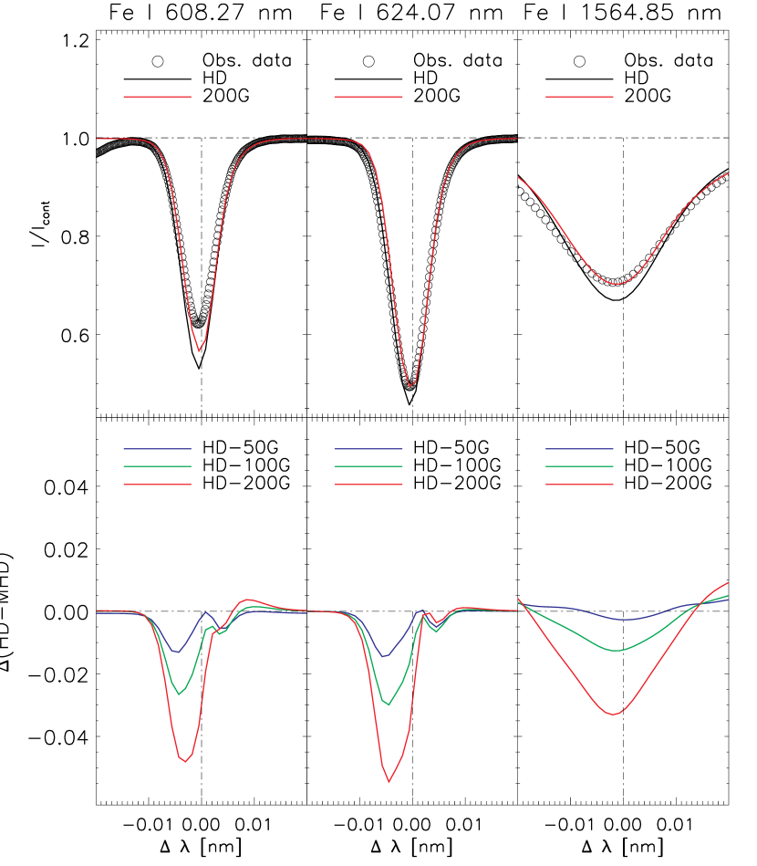
Figure 2: Top panels: normalized theoretical profiles after spatial- and temporal-average for the Fe i $608.27$ nm (left), $624.07$ nm (center) and (right) $1564.85$ nm spectral lines, as derived from the synthesis of relevant spectral regions from the HD and MHD simulations. For the sake of clarity, MHD results are shown only for the simulation with highest magnetic flux. Spectral observational data from the Kitt Peak FTS Spectral Atlas are given for visual comparison (empty circles). Bottom panels: intensity difference between average normalized synthetic line profiles in HD and MHD.

Observational data taken from the FTS spectral atlas (Brault et al., 1987) are also shown in the figure for visual comparison (top panels, empty circles). The fit of the line profiles is satisfactory, with the MHD models performing better than the HD one. In any case, since the objective is a differential analysis between MHD and HD, the scope of the work presented here does not require obtaining extremely high accuracy in the fitting of observed line profiles. Remaining discrepancies in the fitting, especially in the line cores, can be explained by the higher temperatures in the relevant layers of our MHD models, which will lead to stronger neutral iron overionisation and are thus likely to induce larger departures from the LTE assumption adopted here.

More importantly with regards to our aim here, we verified that our equivalent width calculation converged with regards to the number of sampled spectral wavelengths. Moreover, our equivalent-width estimates are in fair agreement with the observational values found in the literature (Gurtovenko & Kostik, 1986; Blackwell, Lynas-Gray, & Smith, 1995; Holweger, Kock, & Bard, 1995; Kostik, Shchukina & Rutten, 1996).

A further check of the goodness of our simulations is possible: we obtain an excellent match between our continuum intensity values and those expected from the literature (see figure 2 of Trujillo Bueno & Shchukina, 2009). For example, in units of erg/(cm² s ster Å), we get Stokes I values of $\sim 3.13\cdot 10^{6}$ (continuum around the Be ii $313.04$ and $313.11$ nm lines), $\sim 4.88\cdot 10^{6}$ (continuum around the Fe i 401.02 nm line), $\sim 2.91\cdot 10^{6}$ (around the Fe i $630.15$ and $630.25$ nm lines) and $\sim 2.43\cdot 10^{6}$ (continuum around the Fe i 700.06 nm line). The latter two values match almost perfectly with the observational data of Ayres, Plymate, & Keller (2006). On the other hand, our UV values, while still agreeing to a good level, may be slightly too high due to our neglect of line haze on continuum at those wavelengths.

We have also used Stokes V polarization signature results (Fig. 1, right panel) to derive Stokes V amplitudes. Depending on the wavelength considered, we find Stokes V average amplitudes (measured in units of Stokes I continuum intensity) of the order of $0.01-0.03\%$ (”100 G” case). This corresponds, when calibrating our Stokes V signals using the weak-field approximation, (e.g Martínez González & Bellot Rubio, 2009), to an average unsigned vertical magnetic flux of the order of $10-50$ G. These numbers are typical for solar internetwork and network regions, as deduced when considering the effect of limited spatial resolution of observations. This result confirms that our simulations are representative of solar quiet regions, a description covering 90 percent of the solar surface.

Regarding limb-darkening, recent work by Pereira, Asplund & Kiselman (2009a) shows that related uncertainties in the simulations play only a minimal role for solar abundances. Our differential approach ensures that the small impact of any discrepancy found against limb darkening measurements can be neglected here.

3.2 Thermal versus magnetic effects

Figure 3 compares the average temperature stratification of the different magnetic runs versus optical depth: the averaging was done on a fixed $\log(\tau_{500})$ scale, and over all snapshots. As seen in the figure, in the relevant layers of formation of the absorption features we consider, $\langle T\rangle$ increases with increasing magnetic flux in the simulations, a result expected from radiation transfer considerations in strong solar magnetic elements Spruit (1976); Schüessler & Solanki (1988).

The formation heights of the relevant lines, for the HD case, are: -0.276 Mm for Fe i $624.07$ nm and -0.229 Mm for Fe i $608.27$ nm (Gurtovenko & Kostik, 1986), and -0.135 Mm for Fe i $1564.85$ nm Shchukina & Trujillo Bueno (2001), which correspond to an optical depth of between $\sim-1.6$ and $\sim-0.7$. As seen in the figure, at these optical depths there is a significant temperature increase in the MHD cases compared to HD. The maximum temperature difference, arises at $\log(\tau_{500})\sim-2.5$, reaching up to $125$ K for the run with average vertical magnetic flux density of $200$ G. Together with the direct effect due to the presence of a magnetic field, this has direct implications for the equivalent width of the average profiles and, thus, for the abundance corrections.

As seen in Fig. 2, the line core tends to get weaker in the MHD cases for all of the Fe lines considered, due to the increased average temperature of the corresponding atmospheric models (Fig. 3). For the two visible lines, this indirect influence on the line formation turns out to be the dominant effect, with the direct effect of the magnetic field on the lines being small. Due to its IR wavelength and large magnetic-sensitivity, the $1564$ nm line experiences instead significant direct Zeeman broadening, which, in terms of resulting equivalent width, goes in the opposite direction of the indirect (core-weakening) effect

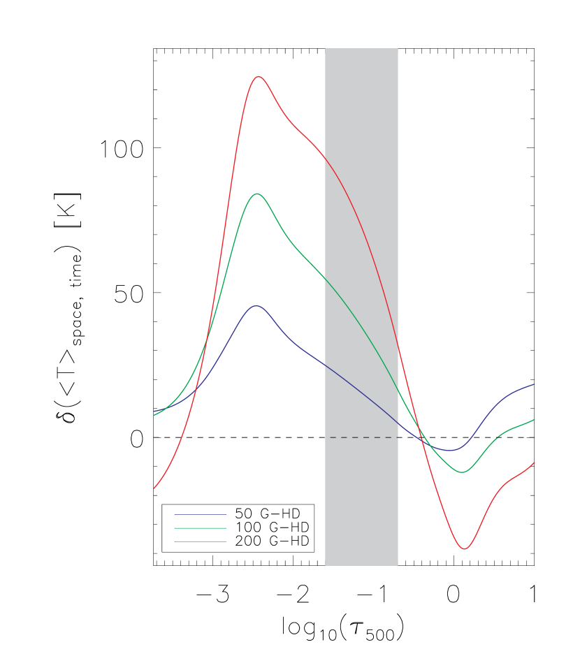
Figure 3: Differences with the HD case in the temperature stratification $\langle T\rangle$ (with averaging taken at fixed optical depth, and over time), for $B_{0}=50$ G (blue line), $100$ G (green line), and $200$ G (red line) cases, plotted against a $log_{10}(\tau_{500})$ scale. The approximate photospheric region of formation for the lines studied is shown with a gray vertical band.

3.3 Differential abundance corrections

Figure 4: Filled circles: derived equivalent widths in the HD run and the three MHD runs, with separate panels for each spectral line. Empty circles: equivalent width in the experiments, when doing the spectral synthesis while setting $B=0$ (leaving the thermodynamics unchanged). The horizontal lines mark the equivalent width for the HD case using the standard solar Fe abundance (solid line), and for iron abundance changes in steps of $|\Delta\log\epsilon_{\odot}(Fe)|=0.01$ dex.

To obtain a differential abundance correction between the HD and MHD cases, we modify the Fe abundance upward or downward of the standard value $\log\epsilon_{\odot}(Fe)=7.50$ (Shchukina & Trujillo Bueno, 2001; Asplund et al., 2009) in the calculation of the average spectra for the HD series. This is done in steps of $0.01$ dex, until the corresponding theoretical equivalent width matches the one derived using the standard iron abundance when computing the average spectra for the MHD case of interest. This method allows us to translate the effects of the magnetic field into abundance corrections.

The equivalent widths of the three spectral lines calculated with the standard Fe abundance are presented in Fig. 4 (filled circles). The figure also gives (dashed horizontal lines) the equivalent width values for the HD case calculated with the iron abundance changed in steps of $0.01$ dex. Since for each case we normalise the average profiles to the relevant continuum level, changes in equivalent width are due to actual changes in the shape and depth of the absorption features. By comparing the filled circles and the horizontal lines in each of the three panels of Fig. 4, we see that the maximum abundance difference is reached in all cases for the runs with the highest field strength, $B=200$ G. The actual numerical values for the maximum difference are: $|\Delta\log\epsilon_{\odot}(Fe)|\sim 0.06$ dex for Fe i $1564.85$ nm; $\sim 0.09$ dex for Fe i $624.07$ nm and slightly above $\sim 0.07$ dex for Fe i $608.27$ nm.

The variations of the equivalent width in Fig. 4 are caused both by direct magnetic effects (i.e., via Zeeman broadening) and, indirectly, via changes in the stratification leading to different amount of absorption in the line core. As the name implies, Zeeman broadening always causes an increase in the equivalent width. In contrast, the indirect contribution resulting from the increased average temperatures in the MHD models is a line-weakening effect for the three chosen lines. This is to be expected (see discussion in Gray, 1992, Chapter 13) for neutral Fe lines in the solar photosphere, where iron is mostly ionized in the relevant layers. One can estimate the relative importance of the direct and indirect effects by ad-hoc setting $B_{0}=0$ while keeping all other variables unmodified when doing the spectral synthesis for the MHD snapshots. The open circles in Fig. 4 show the equivalent widths resulting from carrying out this experiment for all three lines. For the visible lines the indirect effects dominate, which can be expected since they form at heights in the photosphere where the temperature differences between the MHD and HD models become more important. The direct effect for those lines leads to a roughly linear increase of equivalent width with $B$, which is compatible with the Zeeman broadening origin of this effect. For the infrared Fe i $1564.85$ nm line, in turn, the direct magnetic effects become dominant to the point that they reverse the sign of the abundance correction in that case. The sensitivity of this spectral line to the magnetic field is in fact very high, given its longer wavelength and the fact that its Landé factor is g${}_{L}\sim 3$. Also, for this infrared Fe i line there seems to be a saturation effect, although no asymptotic horizontal regime is reached in the range of B used in the present study.

4 Conclusions

In the past decade, an intense debate has arisen due to the conflict created by new solar abundance determinations, see e.g. Asplund (2005), Ayres (2008b), Caffau et al. (2008), Pereira, Kiselman & Asplund (2009), Pereira, Asplund & Kiselman (2009b), Caffau et al. (2010). Despite the fact that the new abundances well match meteoritic values and improve the agreement with solar-neighbourhood and local interstellar-medium abundances, the proposed large reduction of the solar overall metallicity has led to controversies, especially from the helioseismology community, because it spoils the previous agreement between interior sound speed profiles derived from helioseismic measurements and predictions based on the classical solar model (Bahcall et al., 2005; Antia & Basu, 2006).

To settle the open issues, a thorough exploration of the effects on line formation of the interaction between magnetic field and convection is a necessary step. In this letter we have presented a study of that kind using three representative Fe lines. We have determined that magnetic fields have a noticeable influence on the formation of iron lines and consequently on the solar Fe abundance determination. For average vertical flux densities of $200$ G, we obtain abundance corrections (to be applied in order to obtain the same equivalent widths in HD and MHD) between $0.06$ and $0.09$ dex in absolute value, while $|\Delta\log\epsilon_{\odot}(Fe)|\sim 0.05$ dex for all lines for the $100$ G case. A flux density of order $10^{2}$ G, as in the range shown in Fig. 4, is probably the relevant reference value since it has been shown to correspond to the order of the mean field strength of the photospheric plasma (Trujillo Bueno, Shchukina & Asensio Ramos, 2004).

Our results show that the direct (Zeeman) and indirect (stratification-related) effects of the magnetic field contribute in different amounts to the changes in the different lines. The indirect effects cause most of the equivalent width change of the visible Fe lines, with a small contribution from the Zeeman effect; for the infrared line, in contrast, the Zeeman effect is dominant, and in fact changes the sign of the abundance correction. The absolute value of the total correction is similar for all lines, so we can take it as the reference abundance change related with the presence or absence of magnetic field in the convection model. In fact, for the visible lines, the use of MHD models to match the observational data will lead to higher derived iron abundance than when using an HD model, since the predicted theoretical equivalent widths are smaller for the former cases than for the latter. The opposite applies for the Fe i $1564.85$ nm, since the increased temperature of the MHD models is more than compensated by the very large direct Zeeman line splitting.

There are different avenues to explore with a view to confirming and extending all these results. One should consider further reliable Fe I line pairs with different magnetic sensitivity (Vasilyeva & Shchukina, 2010), and carry out an extensive study including all Stokes parameters for the same spectral features as in previous 3D investigations (Shchukina & Trujillo Bueno, 2001; Asplund et al., 2009), but now based on MHD simulations.

On the other hand, spectral synthesis using 3D convection models should aim to match key observational constraints such as spatially resolved line profiles (Pereira, Kiselman & Asplund, 2009; Pereira, Asplund & Kiselman, 2009b), center-to-limb continuum behaviour, calibrated continuum intensities at disk center, spectral energy distribution, and H lines. Finally, it is urgent to explore the magnetic effects in the Sun for lines of other crucial elements.

References

- Antia & Basu (2006) Antia, H. M., & Basu, S. 2006, ApJ, 644, 1292
- Asplund et al. (2000a) Asplund, M., Nordlund, Å., Trampedach, R., Allende Prieto, C., & Stein, R. F. 2000a, A&A, 359, 729
- Asplund et al. (2000b) Asplund, M., Ludwig, H.-G., Nordlund, Å., Stein, R. F. 2000b, A&A, 359, 669
- Asplund (2005) Asplund, M. 2005, ARA&A, 43, 481
- Asplund et al. (2009) Asplund, M., Grevesse, N., Sauval, A. J., & Scott, P. 2009, ARA&A, 47, 481
- Ayres, Plymate, & Keller (2006) Ayres, T. R., Plymate, C., & Keller, C. U. 2006, ApJ, 165, 618
- Ayres (2008a) Ayres, T. R. 2008, ASPC, 384, 52
- Ayres (2008b) Ayres, T. R. 2008, ApJ, 686, 731
- Bahcall et al. (2005) Bahcall, J. N., Basu, S., Pinsonneault, M., & Serenelli, A. M. 2005, ApJ, 618, 1049
- Blackwell, Lynas-Gray, & Smith (1995) Blackwell, D. E., Lynas-Gray, A. E., & Smith, G. 1995, A&A, 296, 217
- Blackwell, Smith, & Lynas-Gray (1995) Blackwell, D. E., Smith, G., & Lynas-Gray, A. E. 1995, A&A, 303, 575
- Borrero (2008) Borrero, J. M. 2008, ApJ, 673, 470
- Brault et al. (1987) Brault, J., & Neckel, H. 1987, Spectral Atlas of the Solar Absolute Disk-averaged and Disk Center Intensity from 3290 Å to 12510 Å (Hamburg: Univ. Hamburg), ftp://nsokp.nso.edu/pub/atlas/
- Caffau et al. (2008) Caffau, E., Ludwig, H.-G., Steffen, M., Ayres, T. R., Bonifacio, P., Cayrel, R., Freytag, B., & Plez, B. 2008, A&A, 488, 1031
- Caffau et al. (2010) Caffau, E., Ludwig, H.-G., Steffen, M., Freytag, B., & Bonifacio, P. 2010, Solar Phys. [arXiv1003.1190]
- Carlsson et al. (2004) Carlsson, M., Stein, R. F., Nordlund, Å., & Scharmer, G. B. 2004, ApJ, 610, L137
- De Pontieu et al. (2006) De Pontieu, B., Carlsson, M., Stein, R., Rouppe van der Voort, L., Löfdahl, M., van Noort, M., Nordlund, Å., & Scharmer, G. 2006, ApJ, 646, 1405
- Dravins et al. (1981) Dravins, D., Lindegren, L., Nordlund, Å. 1981, A&A, 96, 345
- Fabbian et al. (2006) Fabbian, D., Asplund, M., Carlsson, M., & Kiselman, D. 2006, A&A, 458, 899
- Fabbian et al. (2009) Fabbian, D., Asplund, M., Barklem, P. S., Carlsson, M., & Kiselman, D. 2009, A&A, 500, 1221
- Freytag et al. (2002) Freytag, B., Steffen, M., & Dorch, B. 2002, Astron. Nachr., 323, 213
- Gray (1992) Gray, D. F. 1992, ”The observation and analysis of stellar photospheres” (second edition), Camb. Astrophys. Ser., Vol. 20
- Gurtovenko & Kostik (1986) Gurtovenko, E. A. & Kostik, R. I. 1986, Naukova Dumka, Kiev
- Holweger, Kock, & Bard (1995) Holweger, H., Kock, M., & Bard, A. 1995, A&A, 296, 233
- Khomenko et al. (2003) Khomenko, E., Collados, M., Solanki, S. K., Lagg, A. & Trujillo Bueno, J. 2003, A&A, 408, 1115
- Kostik, Shchukina & Rutten (1996) Kostik, R. I., Shchukina, N. G., & Rutten, R. J., 1996, A&A, 305, 325
- Martínez González & Bellot Rubio (2009) Martínez González, M. J. & Bellot Rubio L. R. 2009, ApJ, 700, 1391
- Nordlund (1985) Nordlund, Å., 1985, Solar Phys., 100, 209
- Nordlund & Galsgaard (1995) Nordlund, A. & Galsgaard, K. 1995, Tech. Rep., Astron. Observ., Copenhagen Univ., http://www.astro.ku.dk/ aake/papers/95.ps.gz
- Nordlund, Stein, & Asplund (2009) Nordlund, Å., Stein, R. F.; Asplund, M. 2009, LRSP, 6, 2
- Pereira, Kiselman & Asplund (2009) Pereira, T. M. D., Kiselman, D., & Asplund, M. 2009, A&A, 507, 417
- Pereira, Asplund & Kiselman (2009a) Pereira, T. M. D., Asplund, M., & Kiselman, D. 2009, IAU General Assembly Joint Discussion 10 ”3D views on cool stellar atmospheres: theory meets observation”, (to appear in MmSAI), arXiv0909.4121
- Pereira, Asplund & Kiselman (2009b) Pereira, T. M. D., Asplund, M., & Kiselman, D. 2009, A&A, 508, 1403
- Sánchez Almeida, Emonet & Cattaneo (2003) Sánchez Almeida, J., Emonet, T., & Cattaneo, F. 2003, ApJ, 585, 536
- Sánchez Almeida et al. (2004) Sánchez Almeida, J., Márquez, I., Bonet, J. A., Domínguez Cerdeña, I., Muller, R., 2004, ApJ, 609, L91
- Sánchez Almeida et al. (2010) Sánchez Almeida, J., Bonet, J. A., Viticchié, B., Del Moro, D., 2010, A&A, 715, L26
- Shchukina & Trujillo Bueno (2001) Shchukina, N., & Trujillo Bueno, J. 2001, ApJ, 550, 970
- Shchukina & Trujillo Bueno (2003) Shchukina, N., & Trujillo Bueno, J. 2003, ASPC, 307, 336
- Shelyag et al. (2004) Shelyag, S., Schüssler, M., Solanki, S. K., Berdyugina, S. V., Vögler, A. 2004, ApJ 427, 335.
- Socas-Navarro (2001) Socas-Navarro, H. 2001, ASPC, 236, 487
- Socas-Navarro & Norton (2007) Socas-Navarro, H., & Norton, A. A. 2007, ApJ, 660, L153
- Schüessler & Solanki (1988) Schüessler, M. & Solanki, S. K. 1988, A&A, 192, 338
- Spruit (1976) Spruit, H. C. 1976, Solar Phys., 50, 269
- Stein & Nordlund (2006) Stein, R. F., & Nordlund, Å. 2006, ApJ, 642, 1246
- Stenflo & Lindegren (1977) Stenflo, J. O & Lindegren, L. 1977, A&AS, 59, 367
- Stenflo (1982) Stenflo, J. O. 1982, Solar Phys., 80, 209
- Trujillo Bueno, Shchukina & Asensio Ramos (2004) Trujillo Bueno, J., Shchukina, N., & Asensio Ramos, A. 2004, Nature, 430, 326
- Trujillo Bueno & Shchukina (2009) Trujillo Bueno, J. & Shchukina, N. G., 2009, ApJ, 694, 1364
- Vasilyeva & Shchukina (2010) Vasilyeva, I. E., & Shchukina, N. G. 2010, KPCB, 25, 319
- Vögler et al. (2005) Vögler, A., Shelyag, S., Schüssler, M., Cattaneo, F., Emonet, T., & Linde, T. 2005, A&A, 429, 335