The effect of spin-orbit interaction and attractive Coulomb potential on the magnetic properties of Ga_1-xMn_xAs

Abstract

We employ the dynamical mean-field approximation to study the magnetic properties of a model relevant for the dilute magnetic semiconductors. Our model includes the spin-orbit coupling on the hole bands, the exchange interaction, and the attractive Coulomb potential between the negatively charged magnetic ions and the itinerant holes. The inclusion of the Coulomb potential significantly renormalizes the exchange coupling and enhances the ferromagnetic transition temperature for a wide range of couplings. We also explore the effect of the spin-orbit interaction by using two different values of the ratio of the effective masses of the heavy and light holes. We show that in the regime of small $J_{c}$-$V$ the spin-orbit interaction enhances $T_{c}$, while for large enough values of $J_{c}$-$V$ magnetic frustration reduces $T_{c}$ to values comparable to the previously calculated strong coupling limit.

I Introduction

Although the notion of using magnetic semiconductors in spintronic devices dates back to the 1960’s Baltzer et al. (1966), the discovery of high temperature ferromagnetism in dilute magnetic semiconductors (DMS)Ohno et al. (1996); Munekata et al. (1989) initiated an active search for the optimal compound with a magnetic transition above room temperature. Since these materials are good sources of polarized charge carriers, they may form the basis of future spintronic devices,$\breve{Z}$utić et al. (2004); Wolf et al. (2001) which utilize the spin of the carriers as well as their charge to simultaneously store and process data. Perhaps one of the most promising DMS is GaAs doped with Manganese due to its rather high ferromagnetic transition temperature ($T_{c}>150$ K for bulk samples and $\sim$ 250 K for $\delta$-doped heterostructuresMacDonald et al. (2005); Nazmul et al. (2005)) and its wide use in today’s electronic devices.

In Ga_1-xMn_xAs, the Mn⁺² ion primarily replace Ga⁺³ playing the role of acceptor by introducing an itinerant hole to the p-like valence band. The strong spin-orbit interaction in the valence band couples the angular momentum to the spin of the itinerant hole resulting in total spin $J$=$l+s$=3/2 for the two upper valence bands and $J$=$l-s$=1/2 for the split-off band. Each manganese also introduces a localized spin ($S$=5/2) due to its half-filled $d$ orbital. In addition, since the Mn⁺² ion is negatively charge with respect to the Ga⁺³ ionic background there is an effective attractive interaction between the Mn ion and the charge carriers.

In previous studiesAryanpour et al. (2005); Majidi et al. (2006) some of us have explored the effect of the strong spin-orbit coupling on the ferromagnetic transition temperature $T_{c}$, the carrier polarization as well as the density of states and spectral functions using the Dynamical Mean-Field Approximation (DMFA). In these studies we used the $k\cdot p$ Hamiltonian to model the dispersion of the parent material (GaAs). While $k\cdot p$ is a good approximation around the center of the Brillouin zone ($\Gamma$ point), it is a poor one away from it. In this work we improve our model by incorporating a more realistic tight binding dispersion for the valence bands as well as an attractive on-site potential between the Mn ions and the itinerant holes. Moreover, we study the effect of the spin-orbit interaction of the holes on the magnetic behavior of the DMS. We find that for intermediate values of the exchange coupling both the on-site potential and the spin-orbit enhances the critical temperature, while in the strong coupling regime the spin-orbit interaction significantly suppresses $T_{c}$Moreno et al. (2006).

The effect of the attractive Coulomb potential has been discussed for models with only one valence band, which ignore the spin-orbit interaction,Takahashi and Kubo (2003); Popescu et al. (2007); Calderón et al. (2002); Hwang and Sarma (2005) and multi-band tight-binding models, which include spin-orbit coupling, but with a limited sampling of disorder configurations.Moreo et al. (2007) Here we include on an equal footing the effect of the attractive Coulomb potential using a simple Hartree term, the exchange between magnetic ions and itinerant holes, the spin-orbit coupling, and the disorder within the coherent potential approximation (CPA).Taylor (1967); Soven (1967); Leath and Goodman (1966) We investigate the ferromagnetic transition temperature, the average magnetization of the Mn ions, the polarization of the holes, and the quasiparticle density of states as function of the Coulomb and exchange couplings. First, we use a single band model where spin-orbit interaction is ignored and carriers have angular momenta $J=1/2$. Next, we introduce the spin-orbit coupling in a two-band model with $J=3/2$. By changing the ratio of the masses of the light and heavy bands ($m_{l}$/$m_{h}$) we explore the effect of spin-orbit coupling. This is the minimal model that qualitatively captures the physics of DMS, however, a more realistic approach should incorporate the conduction and split-off bands and this will be discuss in future studies.

II Model

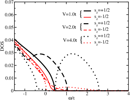
Figure 1: (color online). Spin-dependent density of states for temperature T=0.01t, exchange coupling $J_{c}$=$2\,t$ and Coulomb potential $V=1\,t,2\,t$ and $4\,t$. T=0.01t is below the ferromagnetic transition for all values of $V$.

We employ the simplified Hamiltonian proposed by $\rm{Zar\acute{a}nd}$ and $\rm{Jank\acute{o}}$Zarand and Janko (2002) with an additional Coulomb potential term:

$$H=H_{0}+J_{c}\sum_{i}\mathbf{S}(R_{i})\cdot\mathbf{J}(R_{i})+V\sum_{i}n(R_{i}),$$ (1)

where $H_{0}$ includes both electronic dispersion and spin-orbit coupling of the holes in the parent compound, $J_{c}$ is the exchange coupling, $V$ the Coulomb strength, $\mathbf{S}(R_{i})$, $\mathbf{J}$($R_{i}$) and $n(R_{i})$ are, respectively, the spin of the localized moment, the total angular momentum density and the density of the carriers at random site $i$. Short range direct or superexchange between Mn ions is ignored since we are in the dilute limit and we are not including clustering effects.

As discussed previously,Aryanpour et al. (2005); Majidi et al. (2006) within the DMFA the coarse-grained Green function matrix is:

$$\hat{G}(i\omega_{n})=\frac{1}{N}\sum_{k}[i\omega_{n}\hat{I}-\hat{H}_{0}(k)+\mu\hat{I}-\hat{\Sigma}(i\omega_{n})]^{-1},$$ (2)

where $N$ is the number of $k$ points in the first Brillouin zone, $\mu$ the chemical potential, and $\hat{H}_{0}(k)$ and $\hat{\Sigma}(i\omega_{n})$, are matrices representing the band structure of the parent material and the selfenergy, respectively. The mean field function $\hat{{\cal G}_{0}}(i\omega_{n})=[\hat{G}^{-1}(i\omega_{n})+\hat{\Sigma}(i\omega_{n})]^{-1}$ is required to solve the DMFA impurity problem. At a non-magnetic site, the Green function is simply the mean field function $\hat{G}_{non}(i\omega_{n})=\hat{{\cal G}_{0}}(i\omega_{n})$. The Green function at a magnetic site is $\displaystyle{\hat{G}_{\mathbf{S}}(i\omega_{n})=[{\cal\hat{G}}_{0}^{-1}(i\omega_{n})+J_{c}{\mathbf{S}}\cdot\hat{\mathbf{J}}+V]^{-1}}$ for a given local spin configuration.

Next we average $\hat{G}_{mag}$ over different spin orientation of the local moment. The relatively large magnitude of the Mn moment justifies a classical treatment of its spin. To get the average over the angular distribution we use the effective action Furukawa (1998, 1994)

$$S_{eff}(\mathbf{S})=-\sum_{n}\log\det[\hat{\cal G}_{0}^{-1}(i\omega_{n})+J_{c}{\mathbf{S}}\cdot\hat{\mathbf{J}}+V]e^{i\omega_{n}0^{+}}.$$ (3)

The average over spin configuration is

$$\langle\hat{G}_{mg}(i\omega_{n})\rangle=\frac{1}{Z}\int d\Omega_{\rm{S}}\hat{G}_{\mathbf{S}}(i\omega_{n})\rm{exp[-S_{eff}(\mathbf{S})]},$$ (4)

where $Z$ is the partition function, $Z=\int d\Omega_{\rm\textbf{s}}\rm{exp}(-S_{eff}(\textbf{S}))$. Finally the disorder is treated in a fashion similar to the coherent phase approximation (CPA)Taylor (1967); Soven (1967); Leath and Goodman (1966) and the averaged Green function reads $\hat{G}_{avg}(i\omega_{n})=\langle\hat{G}_{mg}\rangle x+{\cal\hat{G}}_{0}(i\omega_{n})(1-x)$ where $x$ is the doping.

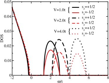
Figure 2: (color online). Spin-dependent density of states for temperature T=0.04t, exchange coupling $J_{c}$=$5\,t$ and various values of the Coulomb potential coupling $V$.

We obtain the hole density of states from the coarse-grained Green function in real frequency domain:

$$\hat{G}(\Omega)=\frac{1}{N}\sum_{k}[\Omega\hat{I}-\hat{H}_{0}(k)-\hat{\Sigma}(\Omega)]^{-1}$$ (5)

where $\Omega=\omega+i0^{+}$. The total density of states (DOS) is

$$DOS(\Omega)=-\frac{1}{\pi}\rm{ImTr\hat{G}(\Omega)},$$ (6)

where Tr is the trace. Each diagonal element of the Green function ($\displaystyle{-\frac{1}{\pi}Im\hat{G}(\Omega)}$) corresponds to the density of states for a specific $J_{z}$ component.

III Results

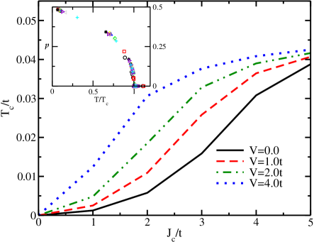
Figure 3: (color online). Ferromagnetic transition temperature versus magnetic exchange coupling for various values of the Coulomb potential. Inset: polarization of the holes as function of $T/T_{c}$ for a wide range of values of $J_{c}$ and $V$. Notice that all the polarization data collapse on a single curve.

Since Ga_1-xMn_xAs is grown using out of equilibrium techniques a noticeable fraction of manganese lies not on the Ga site (substitutional) but on the As site (anti-site) or somewhere in the middle of the crystal structure (interstitial)Jungwirth et al. (2006). The real nature of interstitial defects is still controversial and yet to be resolved, Mašek and Máca (2004); Blinowski and Kacman (2003) but the one consensus is that in most samples there is strong compensation of the holes introduced by substitutional Mn. The density of carriers can also be controlled with electric fields.Ohno et al. (2000) We take these considerations into account by simply setting the filling of the holes to half of the nominal dopingMoreno et al. (2006). We focus on the doping $x$=5% and hole filling of $n_{h}=x/2$.

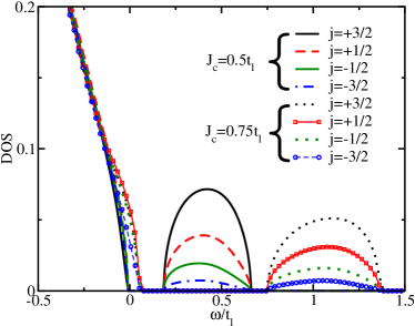
Figure 4: (color online). Density of states for $V$=0. and $J_{c}=$0.5 t_l, T=0.005 t_l; and $J_{c}=$0.75 $t_{l}$ at a temperature T=1/130 t_l. The impurity band is well formed with $J_{c}$=0.5$t_{l}$ and increasing of the coupling shifts the impurity band to higher energies.

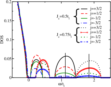
Figure 5: (color online). Density of states for $V$= $t_{l}$, $J_{c}$=0.5 $t_{l}$ T=0.005 t_l; and $J_{c}=$0.75 $t_{l}$ at a temperature T=1/130 t_l. The attractive potential enhances the formation of the impurity band as compared with Fig. 4. The chemical potential lies in the middle of the first impurity band, as it is displayed by the vertical black line.

We start by discussing a simplified one-band model where we ignore the spin-orbit interaction. Our carrier dispersion is $\epsilon_{k}=-2t(\rm{cos}(k_{x})+\rm{cos}(k_{y})+\rm{cos}(k_{z}))$, where $t$ is the spin independent hopping integral. Fig. 1 and 2 display the spin-dependent density of states (DOS) close to the edge of the valence band for coupling constant $J_{c}$=$2\,t$ and $5\,t$, respectively. Note that inclusion of the spin-independent attractive potential results in shifting the energy of the holes (electrons) to lower (higher) energies for both spin species. This is in agreement with previous studies Takahashi and Kubo (2003); Popescu et al. (2007). Fig. 1 illustrates the strong influence of the Hartee term on the states close to the valence band edge for moderate exchange coupling. It is clear that increasing the Coulomb potential accelerates the formation of the impurity band and its splitting from the valence band. Fig. 2 shows that for couplings as large as $J_{c}$=5 $t$ the impurity band is well formed even for relatively small Coulomb potentials ($V$=1 $t$) and the mere effect of the Coulomb term is to shift the impurity band. Notice also that the predicted shift of the impurity band is too large. We believe that this is a consequence of excluding the conduction band from our model, since band repulsion with the conduction band pushes the impurity band to lower energies.

The main panel in Fig. 3 shows the dependency of $T_{c}$ on the exchange coupling for different Coulomb potentials within this simplified one-band model. Comparing this figure with Fig. 1 and 2 it is clear that $T_{c}$ increases as impurity band forms and separates from the edge of the valence band. For each value of $V$ we can identify two values of $J_{c}$ for which the slope of the $T_{c}$ vs. $J_{c}$ curve changes. For $J_{c}<J_{min}$, $T_{c}$ increases very slowly, for $J_{min}<J_{c}<J_{sat}$ the impurity band begins to develop and $T_{c}$ increases with the largest slope, for $J_{c}>J_{sat}$ the impurity band is completely split from the valence band and the rate of increase in $T_{c}$ reduces dramatically. In brief, the appearance of the impurity band corresponds to the large change in the curvature of $T_{c}$ vs. $J_{c}$. After the impurity band is well formed increasing $J_{c}$ or $V$ does not change $T_{c}$ significantly. In fact, for $J_{c}>4\,t$ we can anticipate the saturation of the critical temperature. This is an artifact of the DMFA and is due to the absence of non-local correlations. Inclusion of those correlations leads to magnetic frustration of the system, which in turn suppresses $T_{c}$.Yu et al. (2010); Zarand and Janko (2002) We will come back to this point in more detail later when we discuss the two-band model.

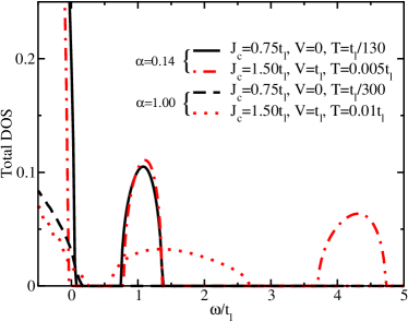
Figure 6: (color online). Density of states for two values of the exchange coupling and Coulomb term: $J_{c}=0.75\,t_{l}$, $V=0$ and $J_{c}=1.5\,t_{l}$, $V=t_{l}$ and temperatures well below the ferromagnetic transition, and for $\alpha$=0.14 and 1.0.

Therefore by increasing the attractive Coulomb potential $T_{c}$ is significantly enhanced for values of the exchange in a given interval, $J_{min}(V)<J_{c}<J_{sat}(V)$, where $J_{min}(V)$ and $J_{sat}(V)$ are function of $V$. This is due mostly to the fact that a positive $V$ promote the appearance of localized states at the magnetic sites which mediate the magnetic order. However, the physics of the ferromagnetic state is not modified by $V$, since the only relevant energy scale is given by $T_{c}$, as one expects from a mean field theory. This is illustrated in the inset of Fig. 3 that displays the polarization of the holes as function of $T/T_{c}$ for a wide range of values of $J_{c}$ and $V$, showing that all the polarization data collapse on a single curve. Thus, the effect of $V$ is just to change the nominal value of $J_{c}$ to a larger $J^{eff}_{c}$.

Now, we introduce a more realistic approach using a two-band model. The spin-orbit interaction and the crystal fields lift the degeneracy of the $p$-like valence bands into heavy, light and split-off bands. In our model we ignore the effect of the split-off band and focus on the heavy and light bands which are degenerate at the center of the Brillouin zone.Luttinger and Kohn (1955) $H_{0}$ is approximated by $\displaystyle H_{0}(k)=\hat{R}^{{\dagger}}(\hat{k})\hat{\epsilon}(k)\hat{R}(\hat{k})\,$, where $\hat{\epsilon}(k)$ is a diagonal matrix with entries $\epsilon(k)_{n,\sigma}=-2t_{n}(\rm{cos}(k_{x})+\rm{cos}(k_{y})+\rm{cos}(k_{z}))$, with $n=l,h$ the heavy/light band index and $\hat{R}(\hat{k})$, the $k\cdot p$ spin $3/2$ rotation matrices.Aryanpour et al. (2005) In GaAs the mass ratio of light and heavy holes at the $\Gamma$ point is $\alpha$=$m_{l}/m_{h}$= 0.14 Yu and Cardona (2001). We compare the results of our simulation for $\alpha$=0.14 and $\alpha$=1, keeping the bandwidth of the light hole band fixed. Furthermore we scale every parameter according to the light holes hopping energy ($t_{l}$), which set the bandwith of the hole band.

Fig. 4 displays the hole density of states close to the edge of the valence band for $J_{c}$= 0.5 $t_{l}$ and 0.75 $t_{l}$ in absence of the Coulomb potential, and for temperatures well below the ferromagnetic transition temperature. One can anticipate that the formation and splitting of the impurity band happens for smaller values of $J_{c}/t_{l}$ than in the one-band model. We can explain this by noting that the total angular momentum of the holes can be as large as $J$=3/2 for heavy holes, leading to a larger contribution to the total energy from the the second term in Eq. (1). Moreover, for a small filling there are more available states close to the center of the Brillouin zone in the two-band model than in the one-band model. Larger number of spin states available to align along the direction of the local moment increases the average exchange energy and favor ferromagnetism.

Fig. 5 displays the density of states for the same exchange couplings and temperatures, $J_{c}$= 0.5 $t_{l}$, T=0.005 t_l, and $J_{c}=$0.75 $t_{l}$, T=1/130 t_l, but with a finite Coulomb potential $V$= $t_{l}$. For these values of the parameters a second impurity band appears in the semiconducting gap. The appearance of two impurity bands is consistent with the fact that the model includes two bands with $J_{z}=\pm 3/2,\pm 1/2$. Notice that the second impurity band is more populated with light holes ($J_{z}=1/2$) while the first impurity band, with higher energy, is mostly made of heavy holes ($J_{z}=3/2$). Since we keep the filling of the holes fixed ($n_{h}$=$x/2$) the chemical potential sits in the middle of the first impurity band, as shown in Fig. 5. Thus, as we discussed previoulsy, the shift of the impurity band will not have noticeable effects on the magnetic properties of the DMS.

To investigate the effect of the spin-orbit interaction we introduce a simple toy model which has all the features of our two-band model except that the heavy and light bands are degenerate over the whole Brillouin zone. Therefore, heavy and light bands have the same dispersion but different total angular momenta $j_{z}$=$\pm$3/2 and $\pm$1/2, respectively. The different band masses introduce magnetic frustrationZarand and Janko (2002); Moreno et al. (2006) and by setting $\alpha$=1.0 ($m_{h}$=$m_{l}$) in our model, this magnetic frustration is removed. Since $t_{l}$ is fixed, changes in $\alpha$ alters the dispersion of the heavy hole band while keeping the light band fixed.

Fig. 6 displays the total DOS for two values of the exchange coupling and Coulomb potential: $J_{c}=0.75\,t_{l}$, $V=0$ and $J_{c}=1.5\,t_{l}$, $V=t_{l}$, and for $\alpha$=0.14 and 1.0. Note that for $\alpha$=0.14 the impurity band is formed at lower couplings. Thus, the spin-orbit interaction enhances the formation of the impurity band. We can explain this by noting that changing $\alpha$ from 1.0 to 0.14 decreases the kinetic energy of the heavy holes (with $j_{z}$=3/2) becoming more susceptible to align their spin parallel to the local moment promoting the formation of the impurity band. Fig. 4 and 5 show explictly that the heavy holes are the majority of the carriers in the impurity band. On the other hand the bandwidth of the impurity band is larger when $\alpha$=1.0, pointing to less localized holes, which better mediate the exchange interaction between magnetic ions.

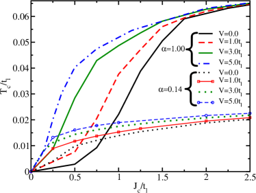
Figure 7: (color online). Ferromagnetic transition temperature, $T_{c}$, vs. exchange coupling $J_{c}$, both in units of $t_{l}$, for different values of the Coulomb potential and for $\alpha$=0.14 and 1.0.

Finally we look at the dependence of the critical temperature on the parameters of the model: $J_{c}$, $V$ and $\alpha$. The results for different values of $J_{c}$-$V$ for $\alpha$=1.0 and 0.14 are shown in Fig. 7. Similarly to Fig. 3 we can identify for both values of $\alpha$ a range of parameters $J_{c}$, $V$ where $T_{c}$ increases strongly. This corresponds to the formation and splitting of the impurity band from the valence band. For small values of $J_{c}$ and $V$, $T_{c}$ is higher for $\alpha=0.14$ but as we increase $J_{c}$-$V$ the ferromagnetic transition temperature for $\alpha=1.0$ becomes larger. Eventually $T_{c}$ saturates due to the lack of non-local correlations within the DMFA. We can understand the higher $T_{c}$ for $\alpha=0.14$ and small $J_{c}$,$V$ by looking at Fig. 6. For $\alpha=0.14$ the impurity band appears at smaller values of $J_{c}$ and $V$ than for $\alpha=1.0$. This is due to the fact that the heavy holes have a smaller kinetic energy and can be polarized more easily and become bonded to the localized moments forming the impurity band. For larger values of $J_{c}$ and $V$, $J_{c}>0.81t_{l}$ for $V=0$, $J_{c}>0.60t_{l}$ for $V=1\,t_{l}$ or $J_{c}>0.29t_{l}$ for $V=3\,t_{l}$, the critical temperature for the model with $\alpha$=1.0 surpasses the one for $\alpha$=0.14 in agreement with previous findings in the strong coupling regimeAryanpour et al. (2005); Moreno et al. (2006). This also can be related with the DOS in Fig. 6, where the bandwith of the impurity band for $\alpha$=1.0 is larger than for $\alpha$=0.14. A larger bandwidth corresponds to weaker localization of the holes and higher mobility. Therefore, they will better mediate the ferromagnetic interaction between the magnetic ions and we expect to see higher $T_{c}$ when $\alpha=1.0$. For the largest value of $J_{c}$ and $V$ we study $T_{c}(\alpha=0.14)/T_{c}(\alpha=1.)=0.35$ to compare with $0.48$ obtained in the strong coupling limitMoreno et al. (2006).

IV Conclusions

In conclusion, we have calculated densities of states, polarizations and ferromagnetic transition temperatures for a one-band and two-band models appropriate for Ga_1-xMn_xAs. We have investigated the effect of adding a local Coulomb attractive potential $V$ between the magnetic ions and the charge carriers. The inclusion of a Coulomb term leads to the formation of the impurity band for smaller magnetic couplings ($J_{c}$), in agreement with previous studiesTakahashi and Kubo (2003); Popescu et al. (2007) and it significantly enhances $T_{c}$ for a wide range of $J_{c}$, without affecting the intrinsic physics of the ferromagnetic transition. We also explore the effect of the spin-orbit interaction by using a two-band model and two different values of the ratio of the effective masses of the heavy and light holes. We show that in the regime of small $J_{c}$-$V$ the spin-orbit interaction enhances $T_{c}$, while for large enough values of $J_{c}$-$V$ the magnetic frustration induced by the spin-orbit coupling reduces $T_{c}$ to values comparable to the previously calculated strong coupling limit.

We acknowledge useful conversation with Randy Fishman and Unjong Yu. This work was supported by the National Science Foundation through OISE-0730290 and DMR-0548011. Computation was carried out at the University of North Dakota Computational Research Center, supported by EPS-0132289 and EPS-0447679.

References

- Baltzer et al. (1966) P. K. Baltzer, P. J. Wojtowicz, M. Robbins, and E. Lopatin, Phys. Rev. 151, 367 (1966).
- Ohno et al. (1996) H. Ohno, A. Shen, F. Matsukura, A. Oiwa, A. Endo, S. Katsumoto, and Y. Iye, Appl. Phys. Lett. 69, 363 (1996).
- Munekata et al. (1989) H. Munekata, H. Ohno, S. von Molnar, A. Segmüller, L. L. Chang, and L. Esaki, Phys. Rev. Lett. 63, 1849 (1989).
- utić et al. (2004) I. utić, J. Fabian, and S. D. Sarma, Rev. Mod. Phys. 76, 323 (2004).
- Wolf et al. (2001) S. A. Wolf et al., Science 294, 1488 (2001).
- MacDonald et al. (2005) A. H. MacDonald, P. Schiffer, and N. Samarth, Nature Materials 4, 195 (2005).
- Nazmul et al. (2005) A. M. Nazmul, T. Amemiya, Y. Shuto, S. Sugahara, and M. Tanaka, Phys. Rev. Lett. 95, 017201/1 (2005).
- Aryanpour et al. (2005) K. Aryanpour, J. Moreno, M. Jarrell, and R. Fishman, Phys. Rev. B 72, 045343/1 (2005).
- Majidi et al. (2006) M. Majidi, J. Moreno, M. Jarrell, R. Fishman, and K. Aryanpour, Phys. Rev. B. 74, 115205/1 (2006).
- Moreno et al. (2006) J. Moreno, R. S. Fishman, and M. Jarrell, Phys. Rev. Lett. 96, 237204/1 (2006).
- Takahashi and Kubo (2003) M. Takahashi and K. Kubo, J. Phys. Soc. Jpn 72, 2866/1 (2003).
- Popescu et al. (2007) F. Popescu, C. Sen, E. Dagotto, and A. Moreo, Phys. Rev. B 76, 85206/1 (2007).
- Calderón et al. (2002) M. J. Calderón, G. Gómez-Santos, and L. Brey, Phys. Rev. B 66, 075218 (2002).
- Hwang and Sarma (2005) E. H. Hwang and S. D. Sarma, Phys. Rev. B. 72, 35210 (2005).
- Moreo et al. (2007) A. Moreo, Y. Yildrim, and G. Alvarez, preprint, arXiv:cond-mat/0710.0577 (2007).
- Taylor (1967) D. Taylor, Phys. Rev. 156, 1017 (1967).
- Soven (1967) P. Soven, Phys. Rev. 156, 809 (1967).
- Leath and Goodman (1966) P. L. Leath and B. Goodman, Phys. Rev. 148, 968 (1966).
- Zarand and Janko (2002) G. Zarand and B. Janko, Phys. Rev. Lett. 89, 047201/1 (2002).
- Furukawa (1998) N. Furukawa, cond-mat/9812066 pp. 1–35 (1998).
- Furukawa (1994) N. Furukawa, J. Phys. Soc. Jpn. 63, 3214/1 (1994).
- Jungwirth et al. (2006) T. Jungwirth, J. Sinova, J. Mašek, J. Kučera, and A. H. MacDonald, Reviews of Modern Physics 78, 809 (2006).
- Mašek and Máca (2004) J. Mašek and F. Máca, Phys. Rev B 69, 165212 (2004).
- Blinowski and Kacman (2003) J. Blinowski and P. Kacman, Phys. Rev. B 67, 121204 (2003).
- Ohno et al. (2000) H. Ohno, D. Chiba, F. Matsukura, T. Omiya, E. Abe, T. Dietl, Y. Ohno, and K. Ohtani, Nature 408, 944 (2000).
- Yu et al. (2010) U. Yu, A.-M. Nili, K. Mikelsons, B. Moritz, J. Moreno, and M. Jarrell, Phys. Rev. Lett. 104, 037201 (2010).
- Luttinger and Kohn (1955) J. M. Luttinger and W. Kohn, Phys. Rev. 97, 869 (1955).
- Yu and Cardona (2001) P. Y. Yu and M. Cardona, Fundamentals of Semiconductors (Springer, 2001).