Polaronic signatures and spectral properties
of graphene antidot lattices

Abstract

We explore the consequences of electron-phonon (e-ph) coupling in graphene antidot lattices (graphene nanomeshes), i.e., triangular superlattices of circular holes (antidots) in a graphene sheet. They display a direct band gap whose magnitude can be controlled via the antidot size and density. The relevant coupling mechanism in these semiconducting counterparts of graphene is the modulation of the nearest-neighbor electronic hopping integrals due to lattice distortions (Peierls-type e-ph coupling). We compute the full momentum dependence of the e-ph vertex functions for a number of representative antidot lattices. Based on the latter, we discuss the origins of the previously found large conduction-band quasiparticle spectral weight due to e-ph coupling. In addition, we study the nonzero-momentum quasiparticle properties with the aid of the self-consistent Born approximation, yielding results that can be compared with future angle-resolved photoemission spectroscopy measurements. Our principal finding is a significant e-ph mass enhancement, an indication of polaronic behavior. This can be ascribed to the peculiar momentum dependence of the e-ph interaction in these narrow-band systems, which favors small phonon momentum scattering. We also discuss implications of our study for recently fabricated large-period graphene antidot lattices.

I Introduction

The discovery of freestanding graphene has spawned huge interest in the electronic and transport properties of this material. Gra (a) In particular, a great deal of research effort is presently being dedicated to graphene-based superlattices. Moi ; Ber (a); Pedersen et al. (2008); Gra (b); Bal Among them, a class of superhoneycomb systems Shima and Aoki (1993) – graphene antidot lattices (graphene nanomeshes Bai et al. (2010)) – was introduced Pedersen et al. (2008) by analogy with the concept of antidot lattices defined atop a two-dimensional electron gas in a semiconductor heterostructure. Sem The electronic, Ant ; Vanević et al. (2009); Fue optical, Ped and magnetic Kin properties of these superlattices result from a subtle interplay of the intrinsic features of graphene and a lattice periodicity imposed by holes (antidots) in a graphene sheet.

Aside from some fundamental aspects, Tworzydło et al. (2006) the main incentive behind the current graphene-related research activity stems from the prospect of a carbon-based electronics. Car Graphene displays exceptional properties, such as room-temperature ballistic transport Müller et al. (2009) on a submicron scale with intrinsic mobility as high as $200,000$ cm²/Vs and the possibility of heavy doping without altering significantly the charge-carrier mobility. Yet, intrinsic semimetallic graphene is of limited utility for fabricating electronic devices Car because the transmission probability of Dirac electrons across a potential barrier is always unity – independent of the height and width of the barrier – a manifestation of Klein tunneling. Kle As a result, the conductivity cannot be controlled through a gate voltage, which, however, is a prerequisite for operation of a conventional field-effect transistor where switching is achieved by gate-voltage induced depletion. Thus it is crucial to open a band gap in graphene. A possible approach entails processing graphene sheets into nanoribbons, which show a confinement-induced gap that scales inversely with their width. To get a gap sufficient for room-temperature transistor operation ($E_{\rm g}\sim 0.5$ eV) one needs ribbons with a width of only few nanometers.

Graphene antidot lattices have a direct electronic band gap stemming from the quantum confinement brought about by the periodic potential of a regular arrangement of antidots. The magnitude of the gap follows a generic scaling relation Kin – a linear increase with the product of the antidot size and density – and can thus be externally controlled. It is this tunability of the band gap – not available when a gap is induced by growing graphene epitaxially on substrates such as SiC – that makes these superlattices interesting from both the fundamental and practical viewpoints. They can be thought of as highly interconnected networks of nanoribbons, and can in principle be fabricated on suspended graphene monolayers via electron-beam lithography, whose current resolution limit is as low as $10$ nm. Yet, being serial in nature, this method is not applicable to large-area patterning of graphene. An alternative fabrication approach, block copolymer lithography, has recently been utilized to fabricate very uniform, free-standing triangular graphene antidot lattices. Bai et al. (2010); Kim et al. (2010) Superior room-temperature electrical properties of the fabricated devices – compared to graphene nanoribbons – have also been demonstrated. Bai et al. (2010)

A thorough understanding of e-ph scattering is of utmost importance because the latter determines the ultimate performance limit of any electronic device: in the high-bias regime of transport the e-ph scattering increases the differential resistance. In the present work, we address the e-ph coupling EPH in graphene antidot lattices and explore some of the ensuing physical consequences. The major e-ph-interaction mechanism in this system, as well as in $\pi$-electron systems in general, SSH (a); Mah ; Non is the modulation of electronic hopping integrals due to lattice distortions (Peierls-type e-ph coupling Pei ).

It is by now widely accepted that e-ph coupling in graphene is comparatively weak: Park et al. (2007); Gra (c) for instance, the angle-resolved photoemission spectroscopy (ARPES) data on inelastic carrier lifetime Bostwick et al. (2007) were consistently explained without even invoking phonon-related effects. Hwang et al. (2007) Here we demonstrate that in graphene antidot lattices, which have completely different band structure than their “parent material”, e-ph coupling is very significant, i.e., properties of these systems undergo a strong phonon-induced renormalization. We ascribe this not only to their narrow-band character and low dimensionality, but also to the peculiar momentum-dependence of the e-ph interaction, favoring small phonon momentum scattering.

Unlike in our recent work, Vukmirović et al. (2010) which was solely concerned with the zero-momentum conduction-band quasiparticle spectral weight for different graphene antidot lattices, in the present work we put an additional emphasis on the directional dependence of the e-ph mass enhancement. This is particularly appropriate because of the anisotropic (in momentum space) character of the relevant e-ph coupling. We also describe the nonzero-momentum spectral properties due to the e-ph coupling at the level of the self-consistent Born approximation. In this way, we obtain results that can be compared with future ARPES measurements.

The outline of the paper is as follows. In Sec. II we introduce the system under consideration, along with the notation and conventions to be used throughout. In subsequent Secs. III and IV we briefly recapitulate the main features of the band structures and phonon spectra of graphene antidot lattices, respectively. Sec. V is set aside for a detailed account of the microscopic mechanism of e-ph coupling in the system, with emphasis on its resulting momentum dependence. The following Sec. VI is devoted to the effect that this momentum-dependence has on the phonon-induced renormalization of electronic properties. In Sec. VII we discuss some implications of our study for optical absorption experiments and charge transport, as well as possible future work. We conclude, with a brief summary of the paper, in Sec. VIII. Some mathematical details are deferred to Appendices A and B.

II Notation and conventions

Triangular graphene antidot lattices with circular antidots are illustrated in Fig. 1. Their geometry is uniquely specified by two dimensionless parameters: the side length of their hexagonal unit cells ($L$) and the antidot radius ($R$), both expressed in units of the graphene lattice constant $a\approx 2.46\>$Å. (Note that $a=a_{cc}\sqrt{3}$, where $a_{cc}=1.42\>$Å  is the distance between nearest-neighbor carbon atoms.) While $L$ is invariably an integer, and defines the superlattice period $La\sqrt{3}$ (center-to-center distance between nearest-neighbor antidots), $R$ can also take non-integer values. Therefore, the notation $\{L,R\}$ will hereafter be used to specify different antidot lattices.

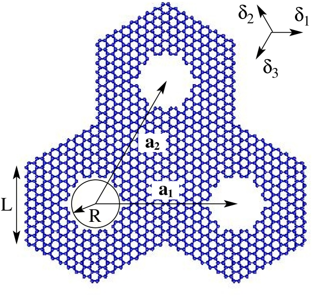
FIG. 1: (Color online) A finite segment of the graphene antidot lattice $\{L,R\}$ with circular antidots. Here $\mathbf{a}_{1}$ and $\mathbf{a}_{2}$ are the superlattice basis vectors; $L$ and $R$ are, respectively, the side length of the hexagonal unit cell and the antidot radius, both expressed in units of the graphene lattice constant $a\approx 2.46\>$Å. The vectors $\bm{\delta}_{1},\>\bm{\delta}_{2}$, and $\bm{\delta}_{3}$ specify positions of the nearest neighbors of a carbon atom on sublattice $A$.

If a carbon atom (henceforth abbreviated as C atom) on sublattice A is taken to be the origin, the adjacent C atoms are determined by the vectors $\bm{\delta}_{1}$, $\bm{\delta}_{2}$, and $\bm{\delta}_{3}$ (see Fig. 1). (For an origin at sublattice B, the corresponding vectors would be $-\bm{\delta}_{1}$,$-\bm{\delta}_{2}$,$-\bm{\delta}_{3}$.)

In what follows, the vectors $\mathbf{R}$ will designate the unit cells ($N$ of them) of an antidot lattice, while $\mathbf{d}_{m}$ ($m=1,\ldots,N_{\textrm{at}}$) will specify the positions of the C atoms within a unit cell. Thus the vectors $\mathbf{R}+\mathbf{d}_{m}$ uniquely specify the positions of all C atoms.

III Band structure of graphene antidot lattices

Much like some other types of graphene-based superlattices, Moi typical antidot lattices contain extremely large numbers of C atoms in their unit cells; in particular, here we consider superlattices with $N_{\textrm{at}}\sim 300-1600$ atoms per unit cell. Such a large system size prohibits the use of methods based on the density functional theory (DFT) for the band-structure and phonon calculations. Instead, we model the band structure using a nearest-neighbor $\pi$-orbital tight-binding model Hamiltonian

$$\hat{H}_{\textrm{e}}=-\frac{t}{2}\sum_{\mathbf{R},m,\bm{\delta}}\big{(}\hat{a}^{\dagger}_{\mathbf{R}+\mathbf{d}_{m}+\bm{\delta}}\hat{a}_{\mathbf{R}+\mathbf{d}_{m}}+\mathop{\rm H.c.}\nolimits\big{)}\>,$$ (1)

where $\hat{a}_{\mathbf{R}+\mathbf{d}_{m}}$ ($\hat{a}^{\dagger}_{\mathbf{R}+\mathbf{d}_{m}}$) destroys (creates) an electron in the $2p_{z}$ orbital ${\varphi}(\mathbf{r}-\mathbf{R}-\mathbf{d}_{m})$ of the C atom located at the position $\mathbf{R}+\mathbf{d}_{m}$, $\bm{\delta}$ stands for the nearest neighbors of that C atom, and $t\approx 2.8$ eV is the nearest-neighbor hopping integral. The tight-binding method is known to be capable of reproducing very accurately the low-energy part of the DFT band structure of graphene. Gra (a) Its accuracy in the case of graphene antidot lattices, i.e., its good agreement with the DFT results for lattices with very small unit cells, has recently been demonstrated. Fue

The Bloch wave functions corresponding to the energy eigenvalues $\varepsilon_{n}(\mathbf{k})$, where $n$ is the band index and $\mathbf{k}$ is a quasimomentum in the Brillouin zone (BZ), are given by

$${\psi}_{n\mathbf{k}}(\mathbf{r})=\sum_{m}C_{m}^{n,\mathbf{k}}{\phi}_{m\mathbf{k}}(\mathbf{r})\>,$$ (2)

where ${\phi}_{m\mathbf{k}}(\mathbf{r})$ is the discrete Fourier transform of $\varphi(\mathbf{r}-\mathbf{R}-\mathbf{d}_{\scriptscriptstyle m})$. Due to the sixfold-rotational point-group symmetry of the system, the coefficients $C^{n,\mathbf{k}}_{m}$ obey the conditions

$$C_{m}^{n,\mathbf{k}}=e^{i\theta(\mathbf{k})}C_{m^{\prime}}^{n,\mathbf{k}^{\prime}}\>,$$ (3)

where $\theta(\mathbf{k})$ is an irrelevant $\mathbf{k}$-dependent phase and $\mathbf{k}^{\prime}$ ($m^{\prime}$) is obtained by rotating the vector $\mathbf{k}$ (atom $m$) through an angle of $\pi/3$.

Unlike graphene itself, graphene antidot lattices show a band structure characteristic of direct band gap semiconductors. In particular, the lattices with circular antidots, that we are concerned with here, fall into the class of superhoneycomb systems (with a unit cell that must have at least the six-fold rotational symmetry) whose possible band structures were classified by Shima and Aoki. Shima and Aoki (1993)

In what follows, we study the $\{L,R=5\}$ ($9\leq L\leq 19$) and $\{L,R=7\}$ ($12\leq L\leq 20$) families of graphene antidot lattices. We find that these lattices are extreme narrow-band systems: for instance, in the $\{L,R=5\}$ family the conduction-electron band width $W_{c}$ is in the range $0.11-0.14$ eV; in the $\{L,R=7\}$ family $W_{c}$ is even smaller ($0.02-0.04$ eV). The band gaps, unlike band widths, decrease with $L$ for given $R$. In the $\{L,R=5\}$ family, they are in the range between $E_{\rm g}=0.146$ eV (for $L=19$) and $E_{\rm g}=0.735$ eV (for $L=9$); in the $\{L,R=7\}$ family, the corresponding range is between $E_{\rm g}=0.118$ eV (for $L=20$) and $E_{\rm g}=0.301$ eV (for $L=12$). The band gap scaling with antidot dimensions was studied in Refs. Ped, and Kin, .

It is worth noting that as a consequence of the bipartite nature of the underlying honeycomb lattice, the resulting energy spectrum of our nearest-neighbor tight-binding model displays particle-hole symmetry. Vanević et al. (2009) This property is not perfectly retained in the exact band structure. Fue

IV Phonon spectra of graphene antidot lattices

The phonon spectrum of graphene was studied extensively, using either DFT methods or effective models. Saito et al. (1998a); Gra (d); Zimmermann et al. (2008); Perebeinos and Tersoff (2009) The effective models are either based on approximating directly the interatomic force constants, with terms that describe coupling of atoms up to some maximum distance, or on adopting an analytic expression for the interaction energy of two or more C atoms. In either case, they contain adjustable parameters whose values are determined by fitting available experimental- and/or DFT data. A well-known class of empirical interatomic potentials for carbon are the Tersoff-Brenner potentials. Bre However, these potentials, with interatomic-interaction range that corresponds only to second-nearest-neighbor distance, do not provide the accuracy typically needed in phonon calculations. Gra (d); Zimmermann et al. (2008) A generalization of these potentials, with interactions up to fourth-nearest-neighbor, was implemented by Tewary and Yang for calculating the phonon spectra and elastic constants of graphene. Gra (d) Yet, this graphene-specific generalization does not lend itself to the use in other carbon-based systems, as the generalized potentials become unstable away from the equilibrium lattice configuration of graphene.

In the present work, we determine the phonon spectra of the $\{L,R=5\}$ and $\{L,R=7\}$ graphene antidot lattices (with the values of $L$ specified above) using two independent models that have recently been shown to yield very accurate results for graphene itself: the fourth-nearest-neighbor force-constant (4NNFC) method Jishi et al. (1993) in the parametrization of Zimmermann et al., Zimmermann et al. (2008) and the valence force-field (VFF) model, developed for graphene by Perebeinos and Tersoff. Perebeinos and Tersoff (2009) These two models belong to the two aforementioned mutually distinct groups of effective lattice-dynamical models. Both models are, in principle, applicable to any $sp^{2}$-hybridized carbon system.

The 4NNFC model, introduced by Saito et al. Saito et al. (1998a), entails a direct parametrization of the real-space force constants up to fourth-order neighbors, hence the name. The model includes a set of $12$ adjustable parameters, whose values are determined by fitting the ab-initio phonon dispersion (for the parameter values, see Table I in Ref. Zimmermann et al., 2008). These force-constant parameters correspond to the radial (bond-stretching), and both in-plane and out-of-plane tangential (bond-bending) directions between an atom and its $n$-th nearest neighbors. The underlying formalism is described in detail in Ref. Saito et al., 1998b.

The VFF model of Perebeinos and Tersoff is based on an explicit expression for the interaction energy, which includes six different contributions, respectively related to: bond-stretching, bending, out-of-plane vibrations, misalignment of neighboring $\pi$ orbitals, bond-order, and coupling between bond stretching and bond bending [see Eqs. (1) and (2) in Ref. Perebeinos and Tersoff, 2009]. Each contribution is parameterized by the corresponding stiffness constant; their values (see Table I in Ref. Perebeinos and Tersoff, 2009) are determined by fitting experimental and ab-initio data for phonon energies and elastic constants. The model makes no reference to any underlying crystal structure; the only restriction to its use is that the local geometry be consistent with $sp^{2}$ bonding, i.e., that the three adjacent C atoms are not too far from being $120^{\circ}$ apart. Perebeinos and Tersoff (2009) Thus the model can be directly applied not only to graphene but also to various other allotropes of carbon, with graphene antidot lattices being an example of such structures.

In each particular case, we first find the equilibrium lattice configuration by relaxing the atoms until the forces on all of them are smaller than $10^{-5}$ eV/Å. We then construct the force-constant tensor

$$D_{m\beta,m^{\prime}\beta^{\prime}}(\mathbf{R}-\mathbf{R}^{\prime})\equiv\frac{\partial^{2}E_{\textrm{tot}}(\{\mathbf{u}_{m}(\mathbf{R})\})}{\partial u_{m\beta}(\mathbf{R})\partial u_{m^{\prime}\beta^{\prime}}(\mathbf{R}^{\prime})}\>,$$ (4)

where $u_{m\beta}(\mathbf{R})$ is the displacement – in direction $\beta$ ($\beta=x,y,z$) from the equilibrium position – of an atom at $\mathbf{R}+\mathbf{d}_{m}$, and $E_{\textrm{tot}}(\{\mathbf{u}_{m}(\mathbf{R})\})$ the total lattice potential energy. The normal-mode frequencies $\omega_{\lambda}(\mathbf{q})$ and eigenvectors $\mathbf{v}^{\lambda}(\mathbf{q})=[\mathbf{v}_{1}^{\lambda}(\mathbf{q}),\ldots,\mathbf{v}_{N_{\textrm{at}}}^{\lambda}(\mathbf{q})]^{T}$ (with $\lambda=1,\ldots,3N_{\textrm{at}}$ enumerating phonon branches) are obtained by solving numerically the secular equation for the dynamical matrix $\mathbf{D}(\mathbf{q})\equiv\sum_{\mathbf{R}}\mathbf{D}(\mathbf{R})\>e^{-i\mathbf{q}\cdot\mathbf{R}}$.

The salient feature of the computed phonon spectra is that the highest optical-phonon energy at $\mathbf{q}=0$ is essentially inherited from graphene itself and thus only weakly dependent on $L$ and $R$. Generally speaking, the comparatively high optical phonon energies in carbon-based systems (graphene, nanotubes, intramolecular modes in fullerides) – which typically extend up to about $200$ meV – are related to the low atomic mass of carbon and to the stiffness of the C-C bond. The energies we obtain for this highest-lying mode in antidot lattices are around $195.3$ meV in the 4NNFC approach and $197.5$ meV in the VFF approach. The highest-energy phonon modes have in common that they do not involve significant displacements in the vicinity of the antidot edges.

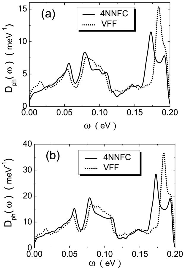
FIG. 2: The phonon density-of-states for the (a) $\{L=9,R=5\}$ and (b) $\{L=13,R=7\}$ graphene antidot lattices, obtained using the 4NNFC (solid line) and VFF (dashed line) methods.

Given the number of phonon modes involved, the most meaningful way of comparing the results of the two methods employed entails calculation of the phonon density-of-states

$$D_{\textrm{ph}}(\omega)\equiv\frac{1}{N}\sum_{\mathbf{q},\lambda}\delta[\omega-\omega_{\lambda}(\mathbf{q})]\>.$$ (5)

This quantity is normalized here such that when integrated over the whole range of $\omega$ it yields the total number of the degrees of freedom per unit cell, i.e., the number of phonon branches $3N_{\textrm{at}}$. In particular, Figs. 2(a) and 2(b) illustrate such a comparison for the $\{L=9,R=5\}$ and $\{L=13,R=7\}$ antidot lattices, respectively. The plots show the qualitative agreement between the two approaches, as well as very similar character of the phonon density-of-states in both families of antidot lattices studied. The accuracy of both methods can potentially be improved as system-specific experimental data become available, allowing to determine more accurately the values of adjustable parameters.

V Electron-phonon coupling in graphene antidot lattices

The dominant e-ph coupling mechanism in $\pi$-electron systems is the modulation of hopping integrals due to lattice distortions, Mah i.e., Peierls-type coupling. Pei The latter forms the basis of the Su-Schrieffer-Heeger (SSH) model. SSH (a, b) In $sp^{2}$-bonded carbon-based systems optical phonons modify the length of the in-plane $\sigma$ bond between two C atoms, thus altering the overlap between the out-of-plane $\pi$ orbitals centered on these atoms. As a result, the $\pi$-electron hopping integrals are dynamically bondlength-dependent; to a linear approximation, they are proportional to the bondlength modulation, with $\alpha=5.27\>\textrm{eV/\AA}$ being the corresponding e-ph coupling constant. Mah ; Vukmirović et al. (2010) The coupling to acoustic phonons, on the other hand, is known to be rather weak in graphene and carbon nanotubes. Park et al. (2007); Borysenko et al. (2010) In our system, where acoustic phonons have even lower energies than in graphene and carbon nanotubes, this coupling is expected to be even weaker and can therefore be safely neglected.

The momentum-space form of the e-ph-coupling Hamiltonian reads

$$\hat{H}_{\textrm{ep}}=\frac{1}{\sqrt{N}}\sum_{\mathbf{k,q},\lambda,nn^{\prime}}\gamma_{nn^{\prime}}^{\lambda}(\mathbf{k,q})\>\hat{a}_{n,\mathbf{k+q}}^{\dagger}\hat{a}_{n^{\prime},\mathbf{k}}(\hat{b}_{-\mathbf{q},\lambda}^{\dagger}+\hat{b}_{\mathbf{q},\lambda})\>,$$ (6)

where $\hat{a}_{n,\mathbf{k}}$ ($\hat{a}_{n,\mathbf{k}}^{\dagger}$) destroys (creates) an electron with quasimomentum $\mathbf{k}$ in the $n$-th Bloch band, and $\gamma_{nn^{\prime}}^{\lambda}(\mathbf{k,q})$ stands for the (bare) e-ph interaction vertex function. Quite generally, $\gamma_{nn^{\prime}}^{\lambda}(\mathbf{k,q})$ has the meaning of the matrix element – between the electronic Bloch states $(n^{\prime},\mathbf{k})$ and $(n,\mathbf{k+q})$ – of the induced self-consistent potential $\Delta U_{\lambda\mathbf{q}}$ per unit displacement along the phonon normal coordinate that corresponds to the mode $\lambda\mathbf{q}$:

$$\gamma_{nn^{\prime}}^{\lambda}(\mathbf{k,q})\equiv\frac{1}{\sqrt{2M\omega_{\lambda}(\mathbf{q})}}\>\langle n^{\prime},\mathbf{k}\>|\Delta U_{\lambda\mathbf{q}}|\>n,\mathbf{k+q}\rangle\>.$$ (7)

In systems where $\Delta U_{\lambda\mathbf{q}}$ can be determined as a by-product of a DFT band-structure calculation (in which case it represents a derivative of the self-consistent Kohn-Sham potential), like for graphene, Park et al. (2007); Borysenko et al. (2010) the last expression incorporates contributions of the phonon mode $\lambda\mathbf{q}$ to all possible e-ph coupling mechanisms. Hence there is no need to assume a particular microscopic e-ph interaction form. Here, however, where such an approach is unfeasible, evaluation of $\gamma_{nn^{\prime}}^{\lambda}(\mathbf{k,q})$ is based on the adopted real-space form of the e-ph coupling written in the tight-binding electron basis. In the case at hand

$$\gamma_{nn^{\prime}}^{\lambda}(\mathbf{k,q})=V_{nn^{\prime}}^{\lambda}(\mathbf{k},\mathbf{q})+W_{nn^{\prime}}^{\lambda}(\mathbf{k},\mathbf{q})\>,$$ (8)

where $V_{nn^{\prime}}^{\lambda}(\mathbf{k},\mathbf{q})$ and $W_{nn^{\prime}}^{\lambda}(\mathbf{k},\mathbf{q})$ are the respective contributions of the neighbors within a single unit cell and those from adjacent unit cells. As shown explicitly in Appendix A,

$$V_{nn^{\prime}}^{\lambda}(\mathbf{k},\mathbf{q})=\frac{\alpha}{\sqrt{8M\omega_{\lambda}(\mathbf{q})}}\sum_{m,\bm{\delta}}\bar{\bm{\delta}}\cdot[\mathbf{v}^{\lambda}_{m+\delta}(\mathbf{q})-\mathbf{v}^{\lambda}_{m}(\mathbf{q})]\\ \times\big{[}(C^{n,\mathbf{k}+\mathbf{q}}_{m+\delta})^{*}C^{n^{\prime},\mathbf{k}}_{m}+(C^{n,\mathbf{k}+\mathbf{q}}_{m})^{*}C^{n^{\prime},\mathbf{k}}_{m+\delta}\big{]}\>,$$ (9)

where $\bar{\bm{\delta}}\equiv\bm{\delta}/\lVert\bm{\delta}\rVert$, while $m+\delta$ denotes neighbors $\mathbf{d}_{m}+\bm{\delta}$ of site $\mathbf{d}_{m}$, and

$$W_{nn^{\prime}}^{\lambda}(\mathbf{k},\mathbf{q})=\frac{\alpha}{\sqrt{8M\omega_{\lambda}(\mathbf{q})}}\sideset{}{{}^{\prime}}{\sum}_{m,\bm{\delta},\mathbf{a}}\bar{\bm{\delta}}\cdot[e^{i\mathbf{q}\cdot\mathbf{a}}\mathbf{v}^{\lambda}_{m_{1}}(\mathbf{q})-\mathbf{v}^{\lambda}_{m}(\mathbf{q})]\\ \times\big{[}e^{-i(\mathbf{k}+\mathbf{q})\cdot\mathbf{a}}(C^{n,\mathbf{k}+\mathbf{q}}_{m_{1}})^{*}C^{n^{\prime},\mathbf{k}}_{m}+e^{i\mathbf{k}\cdot\mathbf{a}}(C^{n,\mathbf{k}+\mathbf{q}}_{m})^{*}C^{n^{\prime},\mathbf{k}}_{m_{1}}\big{]}\>.$$ (10)

The prime on the last sum indicates that the sum is restricted to the neighbors $\mathbf{d}_{m}+\bm{\delta}$ of site $\mathbf{d}_{m}$ that satisfy the condition $\mathbf{d}_{m}+\bm{\delta}=\mathbf{a}+\mathbf{d}_{m_{1}}$ for some $m_{1}=m_{1}(\bm{\delta})$, with $\mathbf{a}=\pm\mathbf{a}_{1}$, $\pm\mathbf{a}_{2}$, $\pm(\mathbf{a}_{1}-\mathbf{a}_{2})$ (see Fig. 1).

For the conduction band ($n\rightarrow c$) electrons, in the absence of interband ($n\neq n^{\prime}$) scattering, the e-ph Hamiltonian of Eq. (6) reduces to the effective form

$$\hat{H}^{(\textrm{c})}_{\textrm{ep}}=\frac{1}{\sqrt{N}}\sum_{\mathbf{k,q},\lambda}\gamma_{\textrm{cc}}^{\lambda}(\mathbf{k,q})\>\hat{a}_{\textrm{c},\mathbf{k+q}}^{\dagger}\hat{a}_{\textrm{c},\mathbf{k}}(\hat{b}_{-\mathbf{q},\lambda}^{\dagger}+\hat{b}_{\mathbf{q},\lambda})\>.$$ (11)

Evaluation of the e-ph vertex functions $\gamma_{\textrm{cc}}^{\lambda}(\mathbf{k,q})$ based on Eqs. (9) and (10) requires the full knowledge of the phonon polarization vectors $\mathbf{v}^{\lambda}_{m}(\mathbf{q})$ and Bloch wave functions, with the latter ones entering through the coefficients $C_{m}^{n=c,\mathbf{k}}$.

VI Phonon-induced renormalization

VI.1 Consequences of the momentum dependence of e-ph coupling

At variance with most other familiar types of e-ph interaction, which are either completely momentum independent (Holstein-type coupling Holstein (1959)) or only weakly phonon-momentum dependent (Fröhlich-type coupling Dev ), Peierls-type coupling depends strongly on both the electron and phonon momenta. This translates into a strongly-retarded nature of the interaction, which can have a variety of physical consequences. zol Due to particular geometry of the system, the momentum dependence of e-ph interaction in the case at hand is clearly more complicated than that of the standard SSH coupling, which is usually studied on monoatomic lattices (one-dimensional, or a two-dimensional square one).

The quantity that characterizes phonon-induced renormalization for conduction-band electrons is the quasiparticle spectral weight due to e-ph coupling, $Z_{c}(\mathbf{k})\equiv|\langle\Psi_{c\mathbf{k}}|\psi_{c\mathbf{k}}\rangle|^{2}$ , where $|\psi_{c\mathbf{k}}\rangle\equiv\hat{a}^{\dagger}_{c\mathbf{k}}|0\rangle_{\textrm{e}}$ is the bare conduction-electron Bloch state (i.e., a common eigenstate of $\hat{H}_{\textrm{e}}$ and the total electron momentum operator $\hat{\mathbf{K}}_{\textrm{e}}\equiv\sum_{n^{\prime},\mathbf{k^{\prime}}}\mathbf{k^{\prime}}\>\hat{a}^{\dagger}_{n^{\prime},\mathbf{k^{\prime}}}\hat{a}_{n^{\prime}\mathbf{k^{\prime}}}$) and $|\Psi_{c\mathbf{k}}\rangle$ that of the coupled e-ph system (i.e., an eigenstate of the full Hamiltonian of the coupled e-ph system and the total crystal momentum operator $\hat{\mathbf{K}}\equiv\sum_{n^{\prime},\mathbf{k^{\prime}}}\mathbf{k^{\prime}}\>\hat{a}^{\dagger}_{n^{\prime},\mathbf{k^{\prime}}}\hat{a}_{n^{\prime},\mathbf{k^{\prime}}}+\sum_{\lambda,\mathbf{q^{\prime}}}\mathbf{q^{\prime}}\>\hat{b}^{\dagger}_{\lambda,\mathbf{q^{\prime}}}\hat{b}_{\lambda,\mathbf{q^{\prime}}}$).

In a recent work, Vukmirović et al. (2010) we evaluated $Z_{\textrm{c}}(0)$ for the $\{L,R=5\}$ and $\{L,R=7\}$ families of lattices, finding a rather strong phonon-induced renormalization $Z_{\textrm{c}}(0)=0.20-0.27$ [i.e., $Z_{\textrm{c}}^{-1}(0)=3.7-5$], compared to graphene Gra (c) where $Z=0.93$ at Dirac points, or larger. Park et al. (2007) These results, with an excellent agreement between the 4NNFC and VFF approaches, seem to suggest that charge carriers acquire polaronic character. In what follows, we analyze in detail the most important phonon modes and momentum dependence of their corresponding e-ph vertex functions.

The largest contribution to the spectral weight ($75-80$ percent in total) comes from the high-energy modes, more precisely two groups of modes centered around $173$ meV and $194$ meV (cf. Fig. 2). These modes have mixed character, being neither purely transverse nor longitudinal. We also note that within the phonon energy intervals that contribute to the spectral weight, the contribution is dominated by a few modes only. For example, in the case of $\{L=13,R=5\}$ [$\{L=15,R=7\}$] lattice only $9$ ($24$) modes are sufficient to provide already $50$ percent of the spectral weight.

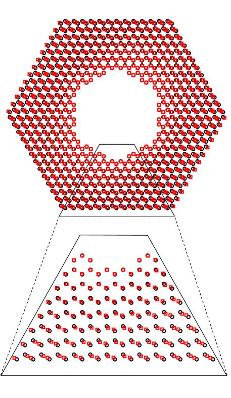
FIG. 3: (Color online) The atomic displacement pattern corresponding to the zone-center phonon mode at energy $E_{\lambda}\approx 197.5$ meV of the $\{L=13,R=5\}$ graphene antidot lattice (top) and its zoomed version (bottom). The displaced (undisplaced) atomic positions are designated by the squares (dark circles).

The highest-energy phonon branches yield the largest individual contribution to $Z_{\textrm{c}}^{-1}(0)$ in all the lattices studied; these contributions are in the range $0.57-0.65$ in the $\{L,R=5\}$ lattices and $0.27-0.34$ in the $\{L,R=7\}$ lattices. Examples of the atomic displacement patterns of such modes for $\{L=13,R=5\}$ and $\{L=15,R=7\}$ antidot lattices are given in Figs. 3 and 4, from which we can infer that these modes do not involve significant atomic displacements in the vicinity of the antidot edges, but only away from them. This is a consequence of the fact that the system is “stiffer” to the displacements of atoms away from edges (which have three neighbors) than those along the edges (only two neighbors). Similar argument explains the dominance of tangential displacements (over radial ones) in the highest-energy phonon modes of fullerides. Gunnarsson (1997)

The last conclusion about the importance of the highest-energy optical phonon branch is similar to that in graphene: based on a first-principles study of the e-ph interaction in graphene, Park et al. Park et al. (2007) concluded that the results could be reproduced by assuming a single Einstein mode at around $200$ meV.

On the other hand, the optical phonons at energies below $30$ meV are far less important than their high-energy counterparts, with their cumulative contribution to the overall spectral weight being at most $20$ percent in the antidot lattices studied. This can already be understood based on the shape of the phonon density-of-states (Fig. 2), from which it is obvious that in the low-energy region the phonon density-of-states is comparatively small.

In order to get a qualitative insight into the obtained results, it is instructive to analyze in detail the underlying e-ph coupling mechanism. The momentum dependence of the bare vertex functions for an electron at the conduction-band bottom ($\mathbf{k}=0$) and the dominant phonon modes in typical lattices is depicted in Figs. 5(a)-(d). What can be inferred from the plots is that the e-ph coupling has a very rich momentum dependence, characterized by a high degree of anisotropy within the irreducible wedge of the BZ. We find several characteristic momentum-space profiles for the coupling functions, some of which correspond to e-ph coupling peaked at (or around) $\mathbf{q}=0$ [Figs. 5(a),(c) and (d)], and the remaining ones to the cases where the latter have maxima at nonzero phonon momenta [Fig. 5(b)].

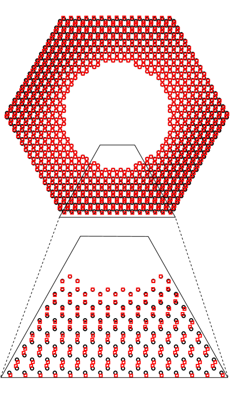
FIG. 4: (Color online) The atomic displacement pattern corresponding to the zone-center phonon mode at energy $E_{\lambda}\approx 197.5$ meV of the $\{L=15,R=7\}$ graphene antidot lattice (top) and its zoomed version (bottom). The displaced (undisplaced) atomic positions are designated by the squares (dark circles).

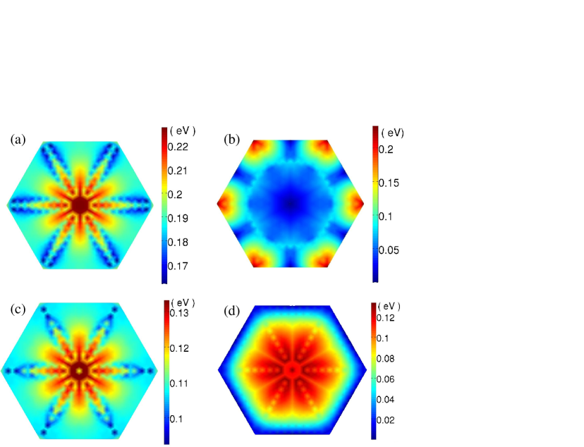
FIG. 5: (Color online) The $\mathbf{q}$-dependence of the moduli $|\gamma^{\lambda}_{\textrm{cc}}(\mathbf{k}=0,\mathbf{q})|$ of the bare e-ph vertex functions, for selected high-energy phonon branches $\lambda$, in the hexagonal Brillouin zones of the $\{L=13,R=5\}$ [(a)-(b)] and $\{L=15,R=7\}$ [(c)-(d)] graphene antidot lattices. The energies of the corresponding optical phonons at $\mathbf{q}=0$, as obtained using the VFF approach, are $E_{\lambda}\approx 197.5$ meV [(a),(c),(d)] and $E_{\lambda}\approx 197.4$ meV [(b)].

In all the cases considered, the coupling to the highest-energy phonon branch is strongest at zero phonon momentum and in its immediate vicinity. The last observation leads us to conclude that the small-phonon-momentum ($\mathbf{q}\approx 0$) scattering involving this mode is to a large extent responsible for the sizeable phonon-induced renormalization that we have obtained. As can be inferred by analyzing the expression for $Z_{\textrm{c}}^{-1}(0)$ in the lowest-order Rayleigh-Schrödinger perturbation theory [Eq. (8) in Ref. Vukmirović et al., 2010], the $\mathbf{q}\approx 0$ terms yield the largest contribution to the relevant integral since for small $\mathbf{q}$ values the denominator of the integrand is very small. The last assertion about the relevance of $\mathbf{q}\approx 0$ scattering is quite general and holds even when the e-ph interaction is completely momentum independent (local in real space), as is the case for Holstein-type interaction. However, our system constitutes an extreme realization of such a physical scenario as the function $|\gamma^{\lambda}_{\textrm{cc}}(\mathbf{k}=0,\mathbf{q})|^{2}$, corresponding to the highest-lying phonon, attains its largest values precisely at $\mathbf{q}=0$ and thus leads to a large mass enhancement. Needless to say, distinct examples of momentum-dependent e-ph interactions do exist where the physical situation is rather different; for the SSH coupling SSH (a); zol $\gamma_{\scriptscriptstyle\textrm{SSH}}(\mathbf{k},\mathbf{q})\propto\sin(\mathbf{k}\cdot\mathbf{a})-\sin\big{[}(\mathbf{k+q})\cdot\mathbf{a}\big{]}$ one has $\gamma_{\scriptscriptstyle\textrm{SSH}}(\mathbf{k}=0,\mathbf{q})\propto|\mathbf{q}|$ at small $\mathbf{q}$. Thus the SSH coupling for $\mathbf{k}=0$ vanishes as $\mathbf{q}\rightarrow 0$. Another familiar example is furnished by the coupling of Zhang-Rice singlets to the “breathing” (oxygen bond-stretching) phonon modes in cuprates, Gun where $\gamma(\mathbf{k},\mathbf{q})=\gamma(\mathbf{q})\propto\sqrt{\sin^{2}(q_{x}/2)+\sin^{2}(q_{y}/2)}$ and is therefore also suppressed at small phonon momenta.

VI.2 Nonzero-momentum spectral properties due to e-ph coupling

In the following, we study nonzero-momentum spectral properties due to e-ph coupling. Because of a considerable computational burden involved, we perform calculations on selected antidot lattices – $\{L=9,R=5\}$ and $\{L=13,R=5\}$ from the $\{L,R=5\}$ family, as well as $\{L=15,R=7\}$ from the $\{L,R=7\}$ family – within the VFF approach.

We determine the conduction-band electron self-energy using the self-consistent Born approximation (SCBA). Gun In the SCBA the electron self-energy is obtained by summing over all the non-crossing diagrams, as illustrated in Fig. 6. Although this approximation neglects e-ph vertex corrections in the self-energy calculation, it yields good results for not-too-strong e-ph coupling. Vuk

FIG. 6: Pictorial representation of the Dyson equation (top). Illustration of the SCBA self-energy, given by a sum over all noncrossing diagrams (bottom).

The SCBA self-energy is given by

$$\Sigma_{\textrm{c}}(\mathbf{k},\omega)=\frac{i}{2\pi N}\sum_{\mathbf{q},\lambda}\int d\Omega\>|\gamma^{\lambda}_{\textrm{cc}}(\mathbf{k},\mathbf{q})|^{2}\\ \times D_{\lambda}(\mathbf{q},\Omega)\>G_{\textrm{c}}(\mathbf{k+q},\omega-\Omega)\>,$$ (12)

where

$$G_{\textrm{c}}(\mathbf{k},\omega) \equiv \frac{1}{\omega-\varepsilon_{\textrm{c}}(\mathbf{k})-\Sigma_{\textrm{c}}(\mathbf{k},\omega)+i\delta}\>,$$ (13)

$$D_{\lambda}(\mathbf{q},\Omega) \equiv \frac{1}{\Omega-\omega_{\lambda}+i0^{+}}-\frac{1}{\Omega+\omega_{\lambda}-i0^{+}}\>,$$ (14)

are the interacting electron and the free phonon propagators, respectively. The frequency integration in Eq. (12) can be carried out explicitly, leading to

$$\Sigma_{\textrm{c}}(\mathbf{k},\omega)=\frac{1}{N}\sum_{\mathbf{q},\lambda}\>|\gamma^{\lambda}_{\textrm{cc}}(\mathbf{k},\mathbf{q})|^{2}\\ \times\frac{1}{\omega-\omega_{\lambda}-\varepsilon_{\textrm{c}}(\mathbf{k}+\mathbf{q})-\Sigma_{\textrm{c}}(\mathbf{k}+\mathbf{q},\omega-\omega_{\lambda})+i\delta}\>.$$ (15)

The last equation is solved self-consistently for electronic (conduction-band) self-energy $\Sigma_{\textrm{c}}(\mathbf{k},\omega)$ using the method of iteration, with the self-energy from Rayleigh-Schrödinger perturbation theory Vukmirović et al. (2010) taken as an initial guess in the iterative process at every $\mathbf{k}$ and $\omega$. The resulting SCBA self-energies for the $\{L=13,R=5\}$ and $\{L=15,R=7\}$ antidot lattices are depicted in Fig. 7(a) and (b), respectively.

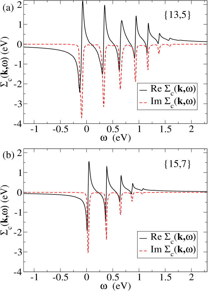
FIG. 7: (Color online) The real and imaginary parts of the SCBA conduction-band electron self-energy in the (a) $\{L=13,R=5\}$ and (b) $\{L=15,R=7\}$ graphene antidot lattices for $\mathbf{k}=0.2\>\mathbf{b}$, where $\mathbf{b}=(0,1)*4\pi/(3La)$.

In this self-energy calculation, a broadening parameter $\delta$ was used, with a value of $5$ meV that corresponds to the resolution of state-of-the-art photoemission experiments. Dam The SCBA electron Green’s function is then evaluated based on Eq. (13), with a typical example shown in Fig. 8. The obtained results are to be compared with future ARPES measurements of the single-particle spectral function $A_{\textrm{c}}(\mathbf{k},\omega)=-\mathop{\rm Im}\nolimits G_{\textrm{c}}(\mathbf{k},\omega)/\pi$.

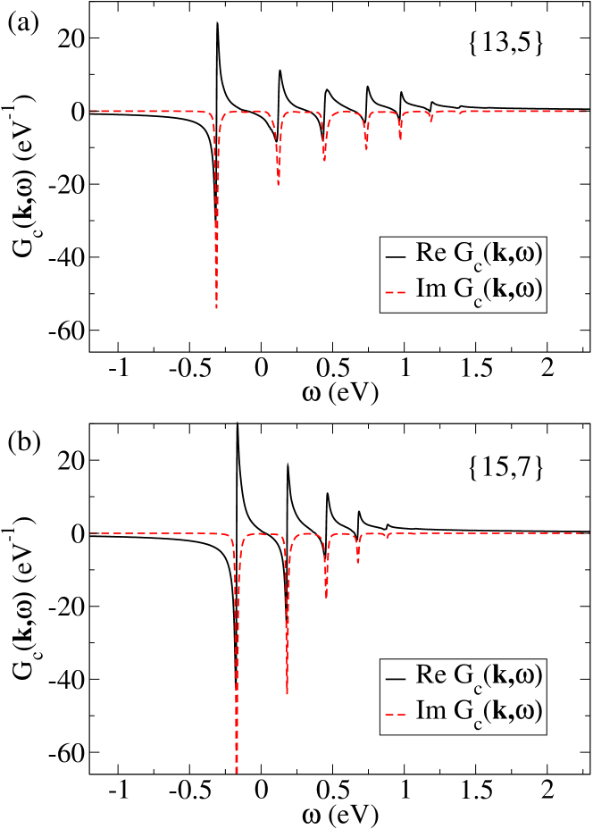
FIG. 8: (Color online) The SCBA electron propagators in the (a) $\{L=13,R=5\}$ and (b) $\{L=15,R=7\}$ graphene antidot lattices for $\mathbf{k}=0.2\>\mathbf{b}$, where $\mathbf{b}=(0,1)*4\pi/(3La)$.

In the case of very weak e-ph interaction the peaks in the spectral function appear at energies that are shifted from the bottom of the dressed-electron band by a characteristic phonon energy. In the case at hand, the positions of peaks result from a complex interplay of multiple phonon modes involved and momentum-dependent e-ph coupling. The fact that the second peak is shifted from the first one by an energy larger than the maximal phonon energy in the system is an additional signature of strong e-ph interaction and polaronic behavior.

The renormalized conduction-band electron dispersion $E_{\textrm{c}}(\mathbf{k})$ is obtained by solving self-consistently the equation Kir

$$E_{\textrm{c}}(\mathbf{k})=\varepsilon_{\textrm{c}}(\mathbf{k})+\mathop{\rm Re}\nolimits\Sigma_{\textrm{c}}[\mathbf{k},E_{\textrm{c}}(\mathbf{k})]\>,$$ (16)

where $\mathop{\rm Re}\nolimits\Sigma_{\textrm{c}}(\mathbf{k},\omega)$ is the real part of the SCBA self-energy. The quasiparticle weight $Z_{\textrm{c}}(\mathbf{k})$ is then computed for different nonzero quasimomenta $\mathbf{k}$ using the standard expression Mahan (1990)

$$Z_{c}(\mathbf{k})=\Big{[}1-\frac{\partial}{\partial\omega}\mathop{\rm Re}\nolimits\Sigma_{c}(\mathbf{k},\omega)\big{|}_{\omega=E_{c}(\mathbf{k})}\Big{]}^{-1}\>.$$ (17)

The obtained values for the $\{L=9,R=5\}$ antidot lattice, for example, are in the range between $0.33$ and $0.37$, all of them being larger than $Z_{\textrm{c}}(\mathbf{k}=0)\approx 0.208$ obtained using Rayleigh-Schrödinger perturbation theory. The increase of the spectral weight away from $\mathbf{k}=0$ is intimately related to the fact that at larger total polaron momentum the momenta of phonons relevant in the scattering process are also larger. Accordingly, the e-ph coupling that predominantly decreases with phonon momentum (recall Sec. VI.1) leads to a smaller renormalization.

In order to characterize the phonon-induced renormalization, it is of interest to determine the direction-dependent e-ph mass enhancement factor

$$\lambda_{\textrm{me}}^{(\alpha)}\equiv\left(\frac{m_{\textrm{eff}}}{m^{*}_{\textrm{e}}}\right)_{\alpha}-1\quad(\alpha=x,y)\>,$$ (18)

where $m_{\textrm{eff}}$ is the effective (in the presence of phonons) and $m^{*}_{\textrm{e}}$ the bare-band mass. Starting from the defining self-consistent relation for the renormalized dispersion [Eq. (16)], it is straightforward to show that (see Appendix B for a derivation consistent with our present notation; alternatively, see Ref. Mahan, 1990)

$$\left(\frac{m_{\textrm{eff}}}{m^{*}_{\textrm{e}}}\right)_{\alpha}=\frac{\displaystyle 1-\frac{\partial}{\partial\omega}\mathop{\rm Re}\nolimits\Sigma_{\textrm{c}}(\mathbf{k},\omega)\big{|}_{\mathbf{k}=0,\omega=E_{\textrm{c}}(0)}}{\displaystyle 1+\frac{\partial}{\partial\varepsilon_{\textrm{c}}(\mathbf{k}_{\alpha})}\mathop{\rm Re}\nolimits\Sigma_{\textrm{c}}(\mathbf{k}_{\alpha},\omega)\big{|}_{\mathbf{k}_{\alpha}=0,\omega=E_{\textrm{c}}(0)}}\>,$$ (19)

where $\mathbf{k}_{\alpha}\equiv(\mathbf{k}\cdot\mathbf{e}_{\alpha})\mathbf{e}_{\alpha}\equiv k_{\alpha}\mathbf{e}_{\alpha}$. It then directly follows that

$$\lambda_{\textrm{me}}^{(\alpha)}=\frac{Z_{\textrm{c}}^{-1}(0)}{\displaystyle 1+\frac{\partial}{\partial\varepsilon_{\textrm{c}}(\mathbf{k}_{\alpha})}\mathop{\rm Re}\nolimits\Sigma_{\textrm{c}}(\mathbf{k}_{\alpha},\omega)\big{|}_{\mathbf{k}_{\alpha}=0,\omega=E_{\textrm{c}}(0)}}-1\>.$$ (20)

The last quantity can be obtained by a numerical differentiation of $\mathop{\rm Re}\nolimits\Sigma_{\textrm{c}}$, using previously obtained values for $Z_{\textrm{c}}^{-1}(0)$. For the $\{L=9,R=5\}$ lattice, our calculations yield the values $\lambda_{\textrm{me}}^{(x)}=2.411$ and $\lambda_{\textrm{me}}^{(y)}=2.448$ [the calculated values of the respective denominators of the fraction in Eq. (20) are 1.4106 and 1.3954]. For the $\{L=13,R=5\}$ lattice we obtain $\lambda_{\textrm{me}}^{(x)}=2.389$ and $\lambda_{\textrm{me}}^{(y)}=2.081$, respectively. In the $\{L=15,R=7\}$ lattice case, we get $\lambda_{\textrm{me}}^{(x)}=1.365$ and $\lambda_{\textrm{me}}^{(y)}=1.255$.

The obtained numbers suggest that the anisotropy in the e-ph mass enhancement is relatively weakly pronounced, despite the existence of anisotropy in the momentum-dependent e-ph coupling [recall Fig. 5]. This can be qualitatively explained by observing that the latter anisotropy of the e-ph coupling is smallest for the highest-energy phonon modes which yield the strongest coupling [for an illustration, note the variation of the values of $|\gamma^{\lambda}_{\textrm{cc}}(\mathbf{k}=0,\mathbf{q})|$ in Fig. 5(a) and (c), as opposed to those in (b) and (d)]. We can therefore draw the conclusion that the overall effective-mass anisotropy in graphene antidot lattices is predominantly determined by the anisotropy of the bare band mass itself, rather than that stemming from phonon-related effects.

VII Discussion

The strong renormalization obtained suggests that the charge carriers in the system acquire polaronic character. Indeed, it is not surprising to have polaronic charge carriers in a narrow-band system. This is a commonplace, for example, in organic semiconductors, such as organic molecular crystals, where narrow electronic bands result from weak van der Waals intermolecular bonding and the e-ph interaction has similar (slightly nonlocal, but still short-ranged) character. Han Compared to these systems, graphene antidot lattices have yet narrower conduction bands (e.g., bare conduction-electron band widths in the polyacene organic crystals can be as large as $700$ meV) and lower dimensionality, both of these factors being conducive to the larger mass enhancement found here.

The strong-coupling regimes in interacting e-ph systems are usually explored using exact diagonalization or variational methods. The criteria for the onset of a (smooth) polaron crossover with the increasing e-ph coupling strength are typically based either on the behavior of the average number of phonons in the polaron ground state – which in the crossover region grows precipitously – or on the behavior of the quasiparticle spectral weight, which in the same regime undergoes a sharp decrease. For a system with short-range, non-polar e-ph interaction (regardless of its concrete form), as is generally the case in covalently-bonded materials such as the one considered here, the polaron crossover has the nature of a change from a quasi-free electron to a small polaron (rather than being a large-to-small polaron crossover, for which a long-range character of the e-ph interaction is a crucial ingredient). However, for a system of such complexity as studied here the use of the aforementioned methods would clearly be inconceivable even with a single “effective” phonon mode, thus the criteria for polaronic behavior cannot be utilized in a strict sense. The perturbative approach is the most powerful technique at our disposal. Obviously, the obtained results are not expected to be valid quantitatively. However, they should still be qualitatively correct, providing an unambiguous evidence for the relevance of phonons in graphene antidot lattices. In addition, it should be stressed that the extent to which the obtained results can be improved is limited: while the accuracy in obtaining the phonon spectra can certainly be improved, due to the prohibitive system size the band structure remains tractable only at the level of the tight-binding method. Finally, even if DFT calculations on such a complex system were feasible, the validity of DFT when calculating e-ph coupling in two-dimensional systems has been called into question. Lazzeri et al. (2008)

An experimental verification of the polaronic nature of carriers in our system should be possible in future optical absorption measurements. Some qualitative predictions can already be made based on general features of (intraband) optical absorption in systems with Peierls-type (SSH) e-ph coupling. Capone et al. (1997) In the polaronic regime, the ground state of such systems is characterized by a shortened bond – being a result of two adjacent sites shifting towards one another – on which the electron is localized. The ground state is then the even combination of the two local electron states. Viewed through simple Franck-Condon-type picture, the optical absorption in such systems proceeds through two different channels: one in which the electron is excited onto another bond (which is not shortened), and the other one in which the electron is excited from the (even-symmetry) ground state to the local odd-symmetry state on the shortened bond itself. The excitation energy in the first process corresponds to the energy gained by the lattice distortion (compared to the undistorted one) and is given by $2E_{\rm p}$, where $E_{\rm p}$ is the polaron binding energy. In the second absorption channel, which corresponds to a transition between a state where the electron energy is lower by $2E_{\rm p}$ with respect to the undistorted lattice to a state where it is higher by the same amount, the excitation energy is twice as large ($4E_{\rm p}$). When the finiteness of the relevant phonon frequency is taken into account, the absorption peaks at energies $2E_{\rm p}$ and $4E_{\rm p}$ from the Franck-Condon picture broaden into bands characterized by phonon features separated by the characteristic phonon energy.

An immediate implication of our results is that the charge transport in graphene antidot lattices – at variance with that of their “parent material” – ought to be modelled by taking into account the inelastic degrees of freedom. This was done previously with carbon nanotubes, Roche et al. (2005) where the inelastic effects in transport are relevant only in the high-bias regime as a consequence of the carrier energy exceeding that of an optical phonon (with energy of $\approx 200$ meV). Car However, in our system there are also optical phonons at far lower energies. Thus the inelastic effects should be even more pronounced than in carbon nanotubes and not necessarily restricted to the high-bias regime.

It is worthwhile noting that the recently fabricated graphene antidot lattices Bai et al. (2010); Kim et al. (2010) comprise even larger number of atoms per unit cell ($N_{\textrm{at}}\gtrsim 5,000$) than the ones discussed here. For comparison, their periods are in the range $27-39$ nm, while the largest period of the superlattices studied here is around $8.2$ nm. Thus it is clearly of interest to extend the present study to such cases. However, a detailed treatment of the e-ph coupling effects, whose complexity scales roughly with $N^{3}_{\textrm{at}}$, for systems of such size would be extremely computationally demanding even with the methodology employed in the present work. Such cases can, however, be addressed within the effective-mass approximation for electronic band structure (wherein the wave functions are expressed through slowly-varying envelope functions) and with a continuum treatment of phonons (deformation potential), an approach well established in other systems. And Knowing that these large-period lattices have larger conduction-band widths (in addition to having smaller band gaps) it is likely that the e-ph coupling effects will be quantitatively less important than in the lattices studied here.

Another important issue for future investigation is the interplay of (short-range) Peierls-type coupling in graphene antidot lattices with the long-range (Fröhlich-type) e-ph coupling at their interface with polarizable substrates such as SiC or SiO₂. Fratini and Guinea (2008) This interplay between the two e-ph coupling mechanisms is likely to be relevant in a field-effect-transistor geometry, where a graphene antidot lattice can be used as the semiconducting channel and SiO₂ as a high-$\kappa$ gate dielectric. Bai et al. (2010) Quite recently, motivated by its relevance in organic field-effect transistors, such interplay has been investigated within a simplified one-dimensional model. DeF The main conclusion of this study was that even a rather weak SSH coupling is sufficient to obtain a polaronic behavior in the simultaneous presence of a moderate polar coupling. In graphene antidot lattices, as a consequence of their different geometry and the ensuing momentum dependence of the e-ph coupling (compared to the genuine SSH coupling; recall discussion in Sec. VI.1) such issues would need to be reconsidered.

VIII Summary and Conclusions

To summarize, we have studied the effects of electron-phonon interaction in graphene antidot lattices. Using realistic band-structure and phonon-spectra calculations as an input, we have described the system based on a model that accounts for the phonon-modulation of electronic hopping integrals – Peierls’ type electron-phonon coupling. We have demonstrated a significant electron-phonon mass enhancement in this system, which is likely to be verified in future ARPES measurements.

The main message of the present work is that in graphene antidot lattices – in contrast to graphene, their parent material – optical phonons, particularly the highest-energy ones, play a very important role. This can be attributed to the narrow-band character of these systems, and, especially, to the peculiar momentum dependence of the relevant electron-phonon interaction which is strongest for small phonon momenta.

Apart from being related to a particular family of graphene-based nanostructured systems of keen current interest, Bai et al. (2010); Kim et al. (2010) our study also bears some fundamental importance. Namely, it provides an insight into the relevance and physical consequences of strongly momentum-dependent electron-phonon interactions. The body of work concerned with such interactions is fairly limited, even at the level of model investigations, Ber (b) in spite of their importance in realistic electronic materials.

The present work bodes well for further studies of graphene antidot lattices, in the finite-temperature case and in the presence of a substrate and/or metallic contacts, Gra (e) all of these aspects being of particular relevance for future room-temperature, carbon-based electronic devices. By providing evidence for the relevance of the inelastic degrees of freedom, our findings are expected to also facilitate future studies of electronic transport in these systems. Detailed investigations of electron-phonon-interaction effects in other emerging classes of graphene-based superlattices Gra (b) are clearly called for.

A Derivation of the electron-phonon-coupling vertex functions

By introducing the matrix $\mathbf{C}_{\mathbf{k}}$ (for each $\mathbf{k}$ in the BZ) such that $C_{m}^{n,\mathbf{k}}=(\mathbf{C}_{\mathbf{k}})_{nm}$, Eq. (2) can be rewritten as

$$\bm{{\psi}}_{\mathbf{k}}(\mathbf{r})=\mathbf{C}_{\mathbf{k}}\bm{{\phi}}_{\mathbf{k}}(\mathbf{r})\>,$$ (A1)

where $\bm{{\psi}}_{\mathbf{k}}(\mathbf{r})\equiv[{\psi}_{n\mathbf{k}}(\mathbf{r})|\>n=1,\ldots,N_{\textrm{at}}]^{T}$ and $\bm{{\phi}}_{\mathbf{k}}(\mathbf{r})\equiv[\phi_{m\mathbf{k}}(\mathbf{r})|\>m=1,\ldots,N_{\textrm{at}}]^{T}$ are $N_{\textrm{at}}$-component vectors. The inverse of the last equation

$$\bm{{\phi}}_{\mathbf{k}}(\mathbf{r})=\mathbf{C}^{-1}_{\mathbf{k}}\bm{{\psi}}_{\mathbf{k}}(\mathbf{r})\>,$$ (A2)

when recast componentwise reads

$${\phi}_{m\mathbf{k}}(\mathbf{r})=\sum_{n}(\mathbf{C}^{-1}_{\mathbf{k}})_{mn}{\psi}_{n\mathbf{k}}(\mathbf{r})\>.$$ (A3)

Given that $C_{m}^{n,\mathbf{k}}$ are the coefficients of a linear transformation [recall Eq. (2)] between two complete orthonormal sets of functions, the matrix $\mathbf{C}_{\mathbf{k}}$ is unitary, so that $(\mathbf{C}^{-1}_{\mathbf{k}})_{mn}=(\mathbf{C}^{\dagger}_{\mathbf{k}})_{mn}=(C_{m}^{n,\mathbf{k}})^{*}$. Consequently, Eq. (A3) is equivalent to

$${\phi}_{m\mathbf{k}}(\mathbf{r})=\sum_{n}(C_{m}^{n,\mathbf{k}})^{*}{\psi}_{n\mathbf{k}}(\mathbf{r})\>,$$ (A4)

and, combined with the inverse Fourier transformation

$${\varphi}(\mathbf{r}-\mathbf{R}-\mathbf{d}_{m})=\frac{1}{\sqrt{N}}\sum_{\mathbf{k}}{\phi}_{m\mathbf{k}}(\mathbf{r})\>e^{-i\mathbf{k}\cdot\mathbf{R}}\>,$$ (A5)

readily implies that

$$\hat{a}^{\dagger}_{\mathbf{R}+\mathbf{d}_{m}}=\frac{1}{\sqrt{N}}\sum_{n,\mathbf{k}}(C_{m}^{n,\mathbf{k}})^{*}e^{-i\mathbf{k}\cdot\mathbf{R}}\hat{a}^{\dagger}_{n\mathbf{k}}\>.$$ (A6)

If, in addition, we assume that for a given vector $\mathbf{d}_{m}$, the vector $\mathbf{d}_{m}+\bm{\delta}$ denotes a site within the same unit cell (i.e., hopping takes place between two lattice sites within the same unit cell), it also holds that

$$\hat{a}_{\mathbf{R}+\mathbf{d}_{m}+\bm{\delta}}=\frac{1}{\sqrt{N}}\sum_{n,\mathbf{k}}C_{m+\delta}^{n,\mathbf{k}}\>e^{i\mathbf{k}\cdot\mathbf{R}}\hat{a}_{n\mathbf{k}}\>.$$ (A7)

From the last two equations, combined with the expression for phonon displacements

$$\hat{\mathbf{u}}_{\lambda,\mathbf{R}+\mathbf{d}_{m}}\equiv\frac{1}{\sqrt{N}}\sum_{\mathbf{q}}\frac{e^{i\mathbf{q}\cdot\mathbf{R}}(\hat{b}^{\dagger}_{-\mathbf{q},\lambda}+\hat{b}_{\mathbf{q},\lambda})}{\sqrt{2M\omega_{\lambda}(\mathbf{q})}}\>\mathbf{v}^{\lambda}_{m}(\mathbf{q})\>,$$ (A8)

we readily obtain

$$\sum_{\mathbf{R}}(\hat{a}^{\dagger}_{\mathbf{R}+\mathbf{d}_{m}+\bm{\delta}}\hat{a}_{\mathbf{R}+\mathbf{d}_{m}}+\mathop{\rm H.c.}\nolimits)\big{[}\hat{\mathbf{u}}_{\lambda,\mathbf{R}+\mathbf{d}_{m}+\bm{\delta}}-\hat{\mathbf{u}}_{\lambda,\mathbf{R}+\mathbf{d}_{m}}\big{]}\cdot\bar{\bm{\delta}}\\ =\frac{1}{\sqrt{N}}\sum_{n,n^{\prime},\mathbf{k},\mathbf{q}}\frac{1}{{\sqrt{2M\omega_{\lambda}(\mathbf{q})}}}\>\bar{\bm{\delta}}\cdot[\mathbf{v}^{\lambda}_{m+\delta}(\mathbf{q})-\mathbf{v}^{\lambda}_{m}(\mathbf{q})]\\ \times\big{[}(C^{n,\mathbf{k}+\mathbf{q}}_{m+\delta})^{*}C^{n^{\prime},\mathbf{k}}_{m}+(C^{n,\mathbf{k}+\mathbf{q}}_{m})^{*}C^{n^{\prime},\mathbf{k}}_{m+\delta}\big{]}\\ \times\hat{a}_{n,\mathbf{k+q}}^{\dagger}\hat{a}_{n^{\prime},\mathbf{k}}(\hat{b}_{-\mathbf{q},\lambda}^{\dagger}+\hat{b}_{\mathbf{q},\lambda})\>.$$ (A9)

The last expression straightforwardly leads to the part of the Hamiltonian in Eq. (6) that corresponds to the hopping within the same unit cell, from which we can read out the expression for $V_{nn^{\prime}}^{\lambda}(\mathbf{k},\mathbf{q})$ in Eq. (9).

If, on the other hand, for a vector $\mathbf{d}_{m}$ in the given unit cell, the nearest-neighbor vector $\mathbf{d}_{m}+\bm{\delta}$ belongs to one of the adjacent unit cells – displaced from the given one by the vector $\mathbf{a}$ [one of the vectors $\pm\mathbf{a}_{1}$, $\pm\mathbf{a}_{2}$, $\pm(\mathbf{a}_{1}-\mathbf{a}_{2})$] – Eq. (A7) ought to be replaced by

$$\hat{a}_{\mathbf{R}+\mathbf{d}_{m}+\bm{\delta}}=\frac{1}{\sqrt{N}}\sum_{n,\mathbf{k}}C_{m_{1}}^{n,\mathbf{k}}e^{i\mathbf{k}\cdot(\mathbf{R}+\mathbf{a})}\hat{a}_{n\mathbf{k}}\>,$$ (A10)

where in the last expression $m_{1}=m_{1}(\bm{\delta})$ ($m_{1}\in\{1,\ldots,N_{\textrm{at}}\}$) is chosen in such a way as to satisfy the condition $\mathbf{d}_{m}+\bm{\delta}=\mathbf{a}+\mathbf{d}_{m_{1}}$. In an analogous manner, the expression for $\hat{\mathbf{u}}_{\lambda,\mathbf{R}+\mathbf{d}_{m}+\bm{\delta}}=\hat{\mathbf{u}}_{\lambda,\mathbf{R}+\mathbf{a}+\mathbf{d}_{m_{1}}}$ should then read [cf. Eq. (A8)]

$$\hat{\mathbf{u}}_{\lambda,\mathbf{R}+\mathbf{d}_{m}+\bm{\delta}}\equiv\frac{1}{\sqrt{N}}\sum_{\mathbf{q}}\frac{e^{i\mathbf{q}\cdot(\mathbf{R}+\mathbf{a})}(\hat{b}^{\dagger}_{-\mathbf{q},\lambda}+\hat{b}_{\mathbf{q},\lambda})}{\sqrt{2M\omega_{\lambda}(\mathbf{q})}}\>\mathbf{v}^{\lambda}_{m_{1}}(\mathbf{q})\>.$$ (A11)

Now, by repeating the steps in the above derivation of the expression for $V_{nn^{\prime}}^{\lambda}(\mathbf{k},\mathbf{q})$, with regard for Eqs. (A10) and (A11), we easily recover expression (10) for $W_{nn^{\prime}}^{\lambda}(\mathbf{k},\mathbf{q})$.

B Derivation of Eq. (19)

We start from the defining self-consistent relation Kir for the renormalized conduction-band electron dispersion:

$$E_{\textrm{c}}(\mathbf{k})=\varepsilon_{\textrm{c}}(\mathbf{k})+\mathop{\rm Re}\nolimits\Sigma_{\textrm{c}}[\mathbf{k},E_{\textrm{c}}(\mathbf{k})]\>.$$ (B1)

By expanding the second term on the right-hand side of the last equation around $\mathbf{k}=0$, we readily obtain

$$E_{\textrm{c}}(\mathbf{k})=\varepsilon_{\textrm{c}}(\mathbf{k})+\mathbf{k}\cdot\frac{\partial}{\partial\mathbf{k}}\mathop{\rm Re}\nolimits\Sigma_{\textrm{c}}(\mathbf{k},\omega)\big{|}_{\mathbf{k}=0,\omega=E_{\textrm{c}}(0)}\\ +E_{\textrm{c}}(\mathbf{k})\frac{\partial}{\partial\omega}\mathop{\rm Re}\nolimits\Sigma_{\textrm{c}}(\mathbf{k},\omega)\big{|}_{\mathbf{k}=0,\omega=E_{\textrm{c}}(0)}+\mathcal{O}(\mathbf{k}^{2})\>,$$ (B2)

which combined with the identity

$$E_{\textrm{c}}(0)=\varepsilon_{\textrm{c}}(0)+\mathop{\rm Re}\nolimits\Sigma_{\textrm{c}}[0,E_{\textrm{c}}(0)]$$ (B3)

leads to the relation

$$\big{[}E_{\textrm{c}}(\mathbf{k})-E_{\textrm{c}}(0)\big{]}\left[1-\frac{\partial}{\partial\omega}\mathop{\rm Re}\nolimits\Sigma_{\textrm{c}}(\mathbf{k},\omega)\big{|}_{\mathbf{k}=0,\omega=E_{\textrm{c}}(0)}\right]\\ =\varepsilon_{\textrm{c}}(\mathbf{k})-\varepsilon_{\textrm{c}}(0)+\mathbf{k}\cdot\frac{\partial}{\partial\mathbf{k}}\mathop{\rm Re}\nolimits\Sigma_{\textrm{c}}(\mathbf{k},\omega)\big{|}_{\mathbf{k}=0,\omega=E_{\textrm{c}}(0)}\\ +\mathcal{O}(\mathbf{k}^{2})\>.$$ (B4)

The mass renormalization in direction $\alpha$ is given by

$$\left(\frac{m_{\textrm{eff}}}{m^{*}_{\textrm{e}}}\right)_{\alpha}=\lim_{\mathbf{k}_{\alpha}\rightarrow 0}\frac{\varepsilon_{\textrm{c}}(\mathbf{k}_{\alpha})-\varepsilon_{\textrm{c}}(0)}{E_{\textrm{c}}(\mathbf{k}_{\alpha})-E_{\textrm{c}}(0)}\>.$$ (B5)

where $\mathbf{k}_{\alpha}\equiv(\mathbf{k}\cdot\mathbf{e}_{\alpha})\mathbf{e}_{\alpha}\equiv k_{\alpha}\mathbf{e}_{\alpha}$. Using the special case $\mathbf{k}=\mathbf{k}_{\alpha}$ of Eq. (B4), after some straightforward manipulations, we finally obtain

$$\left(\frac{m_{\textrm{eff}}}{m^{*}_{\textrm{e}}}\right)_{\alpha}=\frac{\displaystyle 1-\frac{\partial}{\partial\omega}\mathop{\rm Re}\nolimits\Sigma_{\textrm{c}}(\mathbf{k},\omega)\big{|}_{\mathbf{k}=0,\omega=E_{\textrm{c}}(0)}}{\displaystyle 1+\frac{\partial}{\partial\varepsilon_{\textrm{c}}(\mathbf{k}_{\alpha})}\mathop{\rm Re}\nolimits\Sigma_{\textrm{c}}(\mathbf{k}_{\alpha},\omega)\big{|}_{\mathbf{k}_{\alpha}=0,\omega=E_{\textrm{c}}(0)}}\>.$$ (B6)

References

- Gra (a) For a review, see A. H. Castro Neto, F. Guinea, N. M. R. Peres, K. S. Novoselov, and A. K. Geim, Rev. Mod. Phys. , 109 (2009); A. K. Geim, Science , 1530 (2009).
- (2) J. M. B. Lopes dos Santos, N. M. R. Peres, and A. H. Castro Neto, Phys. Rev. Lett. , ().
- Ber (a) C.-H. Park, L. Yang, Y.-W. Son, M. L. Cohen, and S. G. Louie, Nature Phys. , ().
- Pedersen et al. (2008) T. G. Pedersen, C. Flindt, J. Pedersen, N. A. Mortensen, A.-P. Jauho, and K. Pedersen, Phys. Rev. Lett. 100, 136804 (2008).
- Gra (b) A. Isacsson, L. M. Jonsson, J. M. Kinaret, and M. Jonson, Phys. Rev. B , (); H. Sevinçli, M. Topsakal, and S. Ciraci, ibid. , (); Y. P. Bliokh, V. Freilikher, S. Savel’ev, and F. Nori, ibid. , (); L.-G. Wang and S.-Y. Zhu, ibid. , ().
- (6) R. Balog, B. Jørgensen, L. Nilsson, M. Andersen, E. Rienks, M. Bianchi, M. Fanetti, E. Lægsgaard, A. Baraldi, S. Lizzit, Z. Sljivancanin, F. Besenbacher, B. Hammer, T. G. Pedersen, P. Hofmann, and L. Hornekær, Nat. Mater. , ().
- Shima and Aoki (1993) N. Shima and H. Aoki, Phys. Rev. Lett. 71, 4389 (1993).
- Bai et al. (2010) J. Bai, X. Zhong, S. Jiang, Y. Huang, and X. Duan, Nat. Nanotechnol. 5, 190 (2010).
- (9) K. Ensslin and P. M. Petroff, Phys. Rev. B , 12307 (1990); D. Weiss et al., Phys. Rev. Lett. , 2790 (1991).
- (10) T. Shen, Y. Q. Wu, M. A. Capano, L. R. Rokhinson, L. W. Engel, and P. D. Ye, Appl. Phys. Lett. , 122102 (2008).
- Vanević et al. (2009) M. Vanević, V. M. Stojanović, and M. Kindermann, Phys. Rev. B 80, 045410 (2009).
- (12) J. A. Fürst, J. G. Pedersen, C. Flindt, N. A. Mortensen, M. Brandbyge, T. G. Pedersen, and A.-P. Jauho, New J. Phys. , 095020 (2009).
- (13) T. G. Pedersen, C. Flindt, J. Pedersen, A.-P. Jauho, N. A. Mortensen, and K. Pedersen, Phys. Rev. B , (); R. Petersen and T. G. Pedersen, ibid. , ().
- (14) D. Yu, E. M. Lupton, M. Liu, W. Liu, and F. Liu, Nano Res. , 56 (2008); W. Liu, Z. F. Wang, Q. W. Shi, J. Yang, and F. Liu, Phys. Rev. B , 233405 (2009).
- Tworzydło et al. (2006) J. Tworzydło, B. Trauzettel, M. Titov, A. Rycerz, and C. W. J. Beenakker, Phys. Rev. Lett. 96, 246802 (2006).
- (16) See, e.g., P. Avouris, Z. Chen, and V. Perebeinos, Nat. Nanotechnol. , 605 (2007).
- Müller et al. (2009) M. Müller, M. Bräuninger, and B. Trauzettel, Phys. Rev. Lett. 103, 196801 (2009).
- (18) V. V. Cheianov and V. I. Fal’ko, Phys. Rev. B , (2006).
- Kim et al. (2010) M. Kim, N. S. Safron, E. Han, M. S. Arnold, and P. Gopalan, Nano Lett. 10, 1125 (2010).
- (20) See, e.g., F. Marsiglio and J. P. Carbotte, in The Physics of Conventional and Unconventional Superconductors, edited by K. H. Bennemann and J. B. Ketterson (Springer-Verlag, Berlin, 2003), pp. 233–345.
- SSH (a) W. P. Su, J. R. Schrieffer, and A. J. Heeger, Phys. Rev. Lett. , (); Phys. Rev. B , ().
- (22) L. M. Woods and G. D. Mahan, Phys. Rev. B , (2000); G. D. Mahan, ibid. , (2003).
- (23) V. M. Stojanović, P. A. Bobbert, and M. A. J. Michels, Phys. Rev. B , (); C. A. Perroni, E. Piegari, M. Capone, and V. Cataudella, ibid. , ().
- (24) See, for example, K. Yonemitsu and N. Maeshima, Phys. Rev. B , (); V. M. Stojanović and M. Vanević, ibid. , ().
- Park et al. (2007) C.-H. Park, F. Giustino, M. L. Cohen, and S. G. Louie, Phys. Rev. Lett. 99, 086804 (2007).
- Gra (c) J. L. Mañes, Phys. Rev. B , 045430 (2007); M. Calandra and F. Mauri, ibid. , 205411 (2007); T. Stauber, N. M. R. Peres, and A. H. Castro Neto, ibid. , 085418 (2008).
- Bostwick et al. (2007) A. Bostwick, T. Ohta, T. Seyller, K. Horn, and E. Rotenberg, Nature Phys. 3, 36 (2007).
- Hwang et al. (2007) E. H. Hwang, Ben Yu-Kuang Hu, and S. Das Sarma, Phys. Rev. B 76, 115434 (2007).
- Vukmirović et al. (2010) N. Vukmirović, V. M. Stojanović, and M. Vanević, Phys. Rev. B 81, 041408(R) (2010).
- Saito et al. (1998a) R. Saito, T. Takeya, T. Kimura, G. Dresselhaus, and M. S. Dresselhaus, Phys. Rev. B 57, 4145 (1998a).
- Gra (d) J.-A. Yan, W. Y. Ruan, and M. Y. Chou, Phys. Rev. B , (2008); V. K. Tewary and B. Yang, ibid. , 075442 (2009); S. Viola Kusminskiy, D. K. Campbell, and A. H. Castro Neto, ibid. , 035401 (2009).
- Zimmermann et al. (2008) J. Zimmermann, P. Pavone, and G. Cuniberti, Phys. Rev. B 78, 045410 (2008).
- Perebeinos and Tersoff (2009) V. Perebeinos and J. Tersoff, Phys. Rev. B 79, 241409(R) (2009).
- (34) J. Tersoff, Phys. Rev. Lett. , 2879 (); Phys. Rev. B , (); D. W. Brenner, ibid. , ().
- Jishi et al. (1993) R. A. Jishi, L. Venkataraman, M. S. Dresselhaus, and G. Dresselhaus, Chem. Phys. Lett. 209, 77 (1993).
- Saito et al. (1998b) R. Saito, G. Dresselhaus, and M. S. Dresselhaus, Physical Properties of Carbon Nanotubes (Imperial College Press, London, 1998b).
- SSH (b) V. Perebeinos, J. Tersoff, and Ph. Avouris, Phys. Rev. Lett. , 086802 (2005); ibid. , 027402 (2005); L. E. F. Foa Torres and S. Roche, ibid. , 076804 (2006).
- Borysenko et al. (2010) K. M. Borysenko, J. T. Mullen, E. A. Barry, S. Paul, Y. G. Semenov, J. M. Zavada, M. Buongiorno Nardelli, and K. W. Kim, Phys. Rev. B 81, 121412 (2010).
- Holstein (1959) T. Holstein, Ann. Phys. 8, 343 (1959).
- (40) For a recent review, see J. T. Devreese and A. S. Alexandrov, Rep. Prog. Phys. , 066501 (2009).
- (41) M. Zoli, Phys. Rev. B , (); , (); , (); , ().
- Gunnarsson (1997) O. Gunnarsson, Rev. Mod. Phys. 69, 575 (1997).
- (43) O. Gunnarsson and O. Rösch, Phys. Rev. B , 174521 (); J. Phys.: Condens. Matter , 043201 (2008).
- (44) See, for example, N. Vukmirović, Z. Ikonić, D. Indjin, and P. Harrison, Phys. Rev. B , ().
- (45) For a review, see A. Damascelli, Phys. Scr. , 61 ().
- (46) See, e.g., C. Kirkegaard, T. K. Kim, and Ph. Hofmann, New J. Phys. , (); T. Y. Chien, E. D. L. Rienks, M. Fuglsang Jensen, P. Hofmann, and E. W. Plummer, Phys. Rev. B , 241416(R) (2009).
- Mahan (1990) G. D. Mahan, Many-Particle Physics (Plenum Press, New York, 1990).
- (48) K. Hannewald, V. M. Stojanović, and P. A. Bobbert, J. Phys.: Condens. Matter , (); K. Hannewald, V. M. Stojanović, J. M. T. Schellekens, P. A. Bobbert, G. Kresse, and J. Hafner, Phys. Rev. B , (); R. C. Hatch, D. L. Huber, and H. Höchst, ibid. , (); Phys. Rev. Lett. , 047601 (2010).
- Lazzeri et al. (2008) M. Lazzeri, C. Attaccalite, L. Wirtz, and F. Mauri, Phys. Rev. B 78, 081406 (2008).
- Capone et al. (1997) M. Capone, W. Stephan, and M. Grilli, Phys. Rev. B 56, 4484 (1997).
- Roche et al. (2005) S. Roche, J. Jiang, F. Triozon, and R. Saito, Phys. Rev. Lett. 95, 076803 (2005).
- (52) H. Suzuura and T. Ando, Phys. Rev. B , (); T. Ando, J. Phys. Soc. Jpn. , ().
- Fratini and Guinea (2008) S. Fratini and F. Guinea, Phys. Rev. B 77, 195415 (2008).
- (54) G. De Filippis, V. Cataudella, S. Fratini, and S. Ciuchi, e-print arXiv:1005.2476 (2010).
- Ber (b) C. Slezak, A. Macridin, G. A. Sawatzky, M. Jarrell, and T. A. Maier, Phys. Rev. B , 205122 (2006); B. Lau, M. Berciu, and G. A. Sawatzky, ibid. , (); G. L. Goodvin and M. Berciu, ibid. , ().
- Gra (e) S. Barraza-Lopez, M. Vanević, M. Kindermann, and M. Y. Chou, Phys. Rev. Lett. , ().