Crossover distributions at the edge of the rarefaction fan

Abstract

We consider the weakly asymmetric limit of simple exclusion process with drift to the left, starting from step Bernoulli initial data with $\rho_{-}<\rho_{+}$ so that macroscopically one has a rarefaction fan. We study the fluctuations of the process observed along slopes in the fan, which are given by the Hopf–Cole solution of the Kardar–Parisi–Zhang (KPZ) equation, with appropriate initial data. For slopes strictly inside the fan, the initial data is a Dirac delta function and the one point distribution functions have been computed in [Comm. Pure Appl. Math. 64 (2011) 466–537] and [Nuclear Phys. B 834 (2010) 523–542]. At the edge of the rarefaction fan, the initial data is one-sided Brownian. We obtain a new family of crossover distributions giving the exact one-point distributions of this process, which converge, as $T\nearrow\infty$ to those of the Airy $\mathcal{A}_{2\to\mathrm{BM}}$ process. As an application, we prove moment and large deviation estimates for the equilibrium Hopf–Cole solution of KPZ. These bounds rely on the apparently new observation that the FKG inequality holds for the stochastic heat equation. Finally, via a Feynman–Kac path integral, the KPZ equation also governs the free energy of the continuum directed polymer, and thus our formula may also be interpreted in those terms.

and t1Supported by an NSF graduate research fellowship and by PIRE Grant OISE-07-30136. t2Supported by the Natural Science and Engineering Research Council of Canada.

1 Introduction

It is expected that a large class of one-dimensional, asymmetric, stochastic, conservative interacting particle systems/growth models fall into the Kardar–Parisi–Zhang (KPZ) universality class. A manifestation of this is that the KPZ equation should appear as the limit of such systems in the weakly asymmetric limit. The weakly asymmetric limit means to observe the process on space scales of order $\varepsilon^{-1}$ and time scales of order $\varepsilon^{-2}$, while simultaneously rescaling the asymmetry of the model so that it is of order $\varepsilon^{1/2}$. This sort of weak asymmetry zooms in on the critical transition point between the two universality classes associated with growth models—the KPZ class (positive asymmetry) and the Edwards Wilkinson (EW) class (symmetry)—and thus further confirms a mantra of statistical physics that at critical points one expects universal scaling limits.

Bertini and Giacomin BG obtained the first result for the weakly asymmetric simple exclusion process near equilibrium. This is extended to some situations farther from equilibrium in ACQ , directed random polymers in AKQ and partial results are now available GJ for speed changed asymmetric exclusion. In this article we study the situation where asymmetry is to the left and the initial data has an increasing step, so that in the hydrodynamic limit one sees a rarefaction fan. We observe the process along a line $x=vt$ within the fan and study the fluctuations. These converge to the KPZ equation with initial data depending on $v$. For $v$ strictly inside the fan, the initial data is an appropriate scaling of a delta function, and the distribution of the fluctuations is known exactly ACQ , SaSp1 . Our main interest in this article is the fluctuations at the edge of the rarefaction fan. The scaling turns out to be a little different, but the fluctuations are still given by KPZ. Note that since the work of BG it is understood that KPZ is only a formal equation for the fluctuation field and is rigorously defined as the logarithm of the stochastic heat equation. The edge fluctuations correspond to starting the stochastic heat equation with

$$\exp\{-B(X)\}\mathbf{1}_{X>0},$$

where $B(X)$ is a standard Brownian motion in $X$, with $B(0)=0$. We will obtain an exact expression for the one-point probability distribution of the resulting law—the edge crossover distribution—at any positive time. The main tool is the Tracy–Widom determinantal formula for one-sided Bernoulli data, and therefore we are restricted to asymmetric exclusion. The resulting law is expected to be universal for fluctuations at the edge of the rarefaction fan for models in the KPZ class.

1.1 Height function fluctuations at the edge of the rarefaction fan for ASEP

The asymmetric simple exclusion process (ASEP) with parameters $p,q\geq 0$ (such that $p+q=1$) is a continuous time Markov process on the discrete lattice $\mathbb{Z}$ with state space $\{0,1\}^{\mathbb{Z}}$ (the 1s are thought of as particles and the 0s as holes). The dynamics for this process are given as follows: Each particle has an independent exponential alarmclock which rings at rate one. When the alarm goes off, the particle flips a coin, and with probability $p$ attempts to jump one site to the right, and with probability $q$ attempts to jump one site to the left. If there is a particle at the destination, the jump is suppressed, and the alarm is reset (see Liggett for a rigorous construction of this process). If $q=1,p=0$ this process is the totally asymmetric simple exclusion process (TASEP); if $q>p$ it is the asymmetric simple exclusion process (ASEP); if $q=p$ it is the symmetric simple exclusion process (SSEP). Finally, if we introduce a parameter into the model, we can let $q-p$ go to zero with that parameter, and then this class of processes is known as the weakly asymmetric simple exclusion process (WASEP). It is the WASEP, that is, of central interest in this paper since it interpolates between the SSEP and ASEP, and is intimately connected with a stochastic partial differential equation known as the KPZ equation. We denote the asymmetry

$$\gamma=q-p.$$

We consider the family of initial conditions for these exclusion processes which are known of as two-sided Bernoulli and which are parametrized by densities $\rho_{-},\rho_{+}\in[0,1]$. At time zero, each site $x>0$ is occupied with probability $\rho_{+}$, and each site $x\leq 0$ is occupied with probability $\rho_{-}$ (all occupation random variables are independent). These initial conditions interpolate between the step initial condition (where $\rho_{-}=0$ and $\rho_{+}=1$) and the equilibrium or stationary initial condition (where $\rho_{-}=\rho_{+}=\rho$). We will focus on anti-shock initial conditions where $\rho_{-}\leq\rho_{+}$.

Associated to an exclusion process are occupation variables $\eta(t,x)$ which equal 1 if there is a particle at position $x$ at time $t$ and 0 otherwise. From these we define spin variables $\hat{\eta}=2\eta-1$ which take values $\pm 1$ and define the height function for WASEP with asymmetry $\gamma=q-p$ by

$$h_{\gamma}(t,x)=\cases{2N(t)+\displaystyle\sum_{0<y\leq x}\hat{\eta}(t,y),&\quad$x>0,$\vspace*{2pt}\cr 2N(t),&\quad$x=0,$\vspace*{4pt}\cr 2N(t)-\displaystyle\sum_{x<y\leq 0}\hat{\eta}(t,y),&\quad$x<0,$}$$

where $N(t)$ is equal to the net number of particles which crossed from the site 1 to the site 0 in time $t$. Note that at time $t=0$, $h_{\gamma}(0,x)$ is a two-sided simple random walk, with drift $2\rho_{+}-1$ in the positive direction from the origin and drift $2\rho_{-}-1$ in the negative direction.

Proposition 1 ((Hydrodynamic limit))

Let $\rho_{-}\leq\rho_{+}$, $\gamma=\varepsilon^{1/2}$ and $t=\varepsilon^{3/2}$. Then, in probability,

$$\lim_{\varepsilon\rightarrow 0}\frac{h_{\gamma}({t}/{\gamma},vt)}{t}$$

(1)

$$\qquad=\cases{2\rho_{-}(1-\rho_{-})+(2\rho_{-}-1)v,&\quad$\mbox{for }v\leq 2\rho_{-}-1,$\vspace*{2pt}\cr(1+v^{2})/2,&\quad$\mbox{for }v\in[2\rho_{-}-1,2\rho_{+}-1],$\vspace*{2pt}\cr 2\rho_{+}(1-\rho_{+})+(2\rho_{+}-1)v,&\quad$\mbox{for }v\geq 2\rho_{+}-1.$}$$

For $\gamma$ positive and not going to zero with $\varepsilon$, this result is well known Rez91 , TS:1998h . We were not able to find a reference in the weakly asymmetric case. It is an easy consequence of the fluctuation results (i.e., Theorem 16) which make up the main contribution of this paper; see, however, Remark 17.

The region $v\in(2\rho_{-}-1,2\rho_{+}-1)$ is the rarefaction fan, while $v=2\rho_{\pm}-1$ is the edge of the fan. See Figure 1 for an illustration of this limit shape.

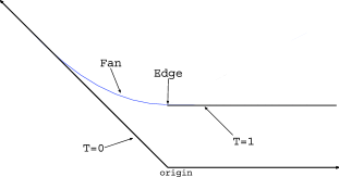
Figure 1: Limit profile for the height function of ASEP with two-sided Bernoulli initial conditions with $\rho_{-}=0$ and $\rho_{+}=1/2$. The rarefaction fan corresponds to velocities $v<0$, and the edge to velocity $v=0$.

For the purposes of this Introduction let us set $\rho_{-}=0$ and $\rho_{+}=1/2$ so that the right edge of the rarefaction fan is at velocity $v=0$. Around this velocity one sees a transition from a curved limit shape for the height function to a flat limit shape. According to (1), the limit height is $t/2$.

Definition 2.

For $m\geq 1$, $\varepsilon>0$, $T>0$ and $X_{1},\ldots,X_{m}\in\mathbb{R}$ set

$$t=\varepsilon^{-3/2}T,\qquad x_{k}=2^{1/3}t^{2/3}X_{k}\quad\mbox{and}\quad\gamma=\varepsilon^{1/2}.$$ (2)

Define the height fluctuation field $h^{\mathrm{fluc}}_{\gamma}(\frac{t}{\gamma},x)$ by

$$h^{\mathrm{fluc}}_{\gamma}\biggl{(}\frac{t}{\gamma},x\biggr{)}:=\frac{h_{\gamma}({t}/{\gamma},x)-{t}/{2}}{t^{1/3}}.$$ (3)

Our first main result is a fluctuation theorem for the WASEP at the edge of the rarefaction fan.

Theorem 3

Let $\rho_{-}=0,\rho_{+}=1/2$ and $h^{\mathrm{fluc}}_{\gamma}(\frac{t}{\gamma},x)$ be the edge fluctuation field defined in Definition 2. Then for $t,\gamma$ and $x$ as in (2), and $h^{\mathrm{fluc}}$ as in (3),

$$\lim_{\varepsilon\rightarrow 0}P\biggl{(}h^{\mathrm{fluc}}_{\gamma}\biggl{(}\frac{t}{\gamma},x\biggr{)}\geq 2^{-1/3}(X^{2}-s)\biggr{)}=F^{\mathrm{edge}}_{T,X}(s),$$

where the edge crossover distribution $F^{\mathrm{edge}}_{T,X}(s)$ is given by

$$F^{\mathrm{edge}}_{T,X}(s)=\int_{\tilde{\mathcal{C}}}e^{-\tilde{\mu}}\frac{d\tilde{\mu}}{\tilde{\mu}}\det(I-K^{\mathrm{edge}}_{s})_{L^{2}(\tilde{\Gamma}_{\eta})}.$$ (4)

The operator $K^{\mathrm{edge}}_{s}$, which depends on $T$ and $X$, and the contour $\tilde{\Gamma}_{\eta}$, $\tilde{\mathcal{C}}$ are defined in Definition 18. Alternative formulas for the distribution function $F^{\mathrm{edge}}_{T,X}(s)$ are given in Section 5.2.

This theorem is proved in Section 3. The proof uses the same method as the proof of the main theorem of ACQ and relies upon a recently discovered exact formula for the probability distribution for the location of a fixed particle in ASEP with step Bernoulli initial conditions (in our case $\rho_{-}=0$ and $\rho_{+}=1/2$). The main technical modification is due to a new infinite product, which we call $g(\zeta)$. Relating this to $q$-Gamma functions we are able to extract the new asymptotic kernel which now also contains Gamma functions.

As we will see in Section 1.2, the $F^{\mathrm{edge}}_{T,X}(s)$ distribution is also the one-point distribution for the KPZ equation (5) with specific initial data (15). It is clear from this result that time and space scale differently. Specifically, the ratio of the scaling exponents for time${}\dvtx{}$space${}\dvtx{}$fluctuations is $3\dvtx 2\dvtx 1$. This scaling ratio was shown in CFP10b to hold for a wide class of $1+1$ dimensional growth models. Finally, the $X^{2}$ shift with respect to the $s$ variable reflects the parabolic curvature of the rarefaction fan nearby the edge.

The above result should be compared (see Section 2.1) with the existing fluctuation theory for TASEP and ASEP. In those cases, using the same centering and scaling as in (3), BBP , BAC and TW4 (resp., for TASEP and ASEP) obtained formulas for the one-point probability distribution function. These formulas actually first arose in the study of the largest eigenvalue of rank one perturbations of complex Wishart random matrix ensembles BBP . Remarkably, the limiting distributions are the same regardless of the asymmetry $\gamma$, as long as it is held positive as the other variables scale to infinity. By scaling $\gamma$ as above, we focus in on the crossover between the ASEP and the SSEP and the new family of edge crossover distribution functions represent this transition.

For TASEP, Corwin, Ferrari and Péché CFP gave a formula for the asymptotic equal time height function fluctuation process (in terms of finite dimensional distributions). We paraphrase this as Theorem 15. For our present case, it says that if we fix $\gamma=1$, $m\geq 1$ (the case $m=1$ is just the BBP , BAC result mentioned above), then for any choices of $T>0$, $X_{1},\ldots,X_{m}\in\mathbb{R}$ and $s_{1},\ldots,s_{m}\in\mathbb{R}$,

$$\lim_{\varepsilon\rightarrow 0}P\Biggl{(}\bigcap_{k=1}^{m}\biggl{\{}h_{\gamma}^{\mathrm{fluc}}\biggl{(}\frac{t}{\gamma},x_{k}\biggr{)}\geq 2^{-1/3}(X_{k}^{2}-s_{k})\biggr{\}}\Biggr{)}=P\Biggl{(}\bigcap_{k=1}^{m}\{\mathcal{A}_{2\to\mathrm{BM}}(X_{k})\leq s_{k}\}\Biggr{)},$$

where $\mathcal{A}_{2\to\mathrm{BM}}$ is a spatial process (defined below in Definition 20) which interpolates between the $\mathrm{Airy}_{2}$ process and Brownian motion.

Since in WASEP we scale the asymmetry with time and space in a critical way, the fluctuation distributions are not the same as for TASEP or ASEP. Rather than having $\gamma=\varepsilon^{1/2}$, one could perform asymptotics with $\gamma=\alpha\varepsilon^{1/2}$. Doing this, it becomes apparent that increasing $T$ is like increasing $\alpha$; hence, one expects to recover the TASEP distributions from the WASEP edge crossover distributions as $T\nearrow\infty$.

Conjecture 4

Let $\rho_{-}=0,\rho_{+}=1/2$, as well as $t,\gamma,x$ and $h^{\mathrm{fluc}}_{\gamma}(\frac{t}{\gamma},x)$ be as in Definition 2. Then for any $m\geq 1$,

$$\lim_{T\rightarrow\infty}\lim_{\varepsilon\rightarrow 0}P\Biggl{(}\bigcap_{k=1}^{m}\biggl{\{}h_{\gamma}^{\mathrm{fluc}}\biggl{(}\frac{t}{\gamma},x_{k}\biggr{)}\geq 2^{-1/3}(X_{k}^{2}-s_{k})\biggr{\}}\Biggr{)}$$

$$\qquad=P\Biggl{(}\bigcap_{k=1}^{m}\{\mathcal{A}_{2\to\mathrm{BM}}(X_{k})\leq s_{k}\}\Biggr{)},$$

where the joint distribution for the process $\mathcal{A}_{2\to\mathrm{BM}}$ is given in Definition 20 in terms of a Fredholm determinant.

Extracting asymptotics from the result of Theorem 3, we are able to confirm this conjecture in the case of $m=1$ (see Section 5.1 for the proof):

Corollary 5

The $F_{T,X}^{\mathrm{edge}}$ distribution has a long time limit which is given by

$$\lim_{T\rightarrow\infty}F^{\mathrm{edge}}_{T,X}(s)=P\bigl{(}\mathcal{A}_{2\to\mathrm{BM}}(X)\leq s\bigr{)},$$

where the above one-point function for the $\mathcal{A}_{2\to\mathrm{BM}}$ process coincides with the so-called BBP-transition BBP in the study of perturbed Wishart random matrices and is given in Definition 20.

Thus by rescaling the edge crossover distribution for WASEP, we recover the universal distribution at the edge of the rarefaction fan for TASEP and ASEP. In the other direction we can also extract the small $T$ asymptotics, which are Gaussian. This is best stated in terms of the stochastic heat equation so we delay it to Proposition 11.

1.2 KPZ equation as the limit for WASEP height function fluctuations at the edge

Following the approach of BG , we prove that as $\varepsilon$ goes to zero, a slight variant on the fluctuation field $h^{\mathrm{fluc}}_{\gamma}(\frac{t}{\gamma},x)$ converges to the KPZ equation with appropriate initial data.

The KPZ equation was introduced by Kardar, Parisi and Zhang in 1986 as arguably the simplest stochastic PDE which contained terms to account for the desired behavior of one-dimensional interface growth KPZ .

$$\partial_{T}\mathcal{H}=-\tfrac 12(\partial_{X}\mathcal{H})^{2}+\tfrac 12\partial_{X}^{2}\mathcal{H}+\dot{\mathscr{W}},\vspace*{-1pt}$$ (5)

where $\dot{\mathscr{W}}(T,X)$ is space–time white noise (see ACQ , Section 1.4, for a rigorous definition of white noise)

$$E[\dot{\mathscr{W}}(T,X)\dot{\mathscr{W}}(S,Y)]=\delta(T-S)\delta(Y-X).\vspace*{-1pt}$$

Despite its simplicity, the KPZ equation has resisted analysis for quite some time. The reason is that, even for nice initial data, the solution at a later time $T>0$ will look locally like a Brownian motion in $X$. Hence the nonlinear term is ill-defined.

In order to make sense of this KPZ equation, we follow BG and simply define the Hopf–Cole solution to the KPZ equation as

$$\mathcal{H}(T,X)=-\log\mathcal{Z}(T,X),\vspace*{-1pt}$$ (6)

where $\mathcal{Z}(T,X)$ is the well-defined W solution of the stochastic heat equation,

$$\partial_{T}\mathcal{Z}=\tfrac 12\partial_{X}^{2}\mathcal{Z}-\mathcal{Z}\dot{\mathscr{W}}.\vspace*{-1pt}$$ (7)

Starting (5) with initial data $\mathcal{H}(0,X)$ means starting (7) with initial data $\mathcal{Z}(0,X)=\exp\{-\mathcal{H}(0,X)\}$. However, one is best advised not to think in terms of $\mathcal{H}$ for the initial data since here we will deal with initial data for $\mathcal{Z}$ (such as Dirac-delta functions) which do not have a well-defined logarithm.

The stochastic partial differential equation (7) is shorthand for its integral version,

$$\mathcal{Z}(T,X) = \int_{-\infty}^{\infty}p(T,X-X_{0})\mathcal{Z}(0,X)\,dX_{0}$$

$${}-\int_{0}^{T}\int_{-\infty}^{\infty}p(T-T_{1},X-X_{1})\mathcal{Z}(T_{1},X_{1})\mathscr{W}(dX_{1}\,dT_{1}),\vspace*{-1pt}$$

where $p(T,X)=(2\pi T)^{-1/2}\exp\{-X^{2}/2T\}$ is the heat kernel. Iterating, one obtains the chaos expansion (convergent in $\mathscr{L}^{2}$ of the white noise $\mathscr{W}$)

$$\mathcal{Z}(T,X)=\sum_{n=0}^{\infty}(-1)^{n}I_{n}(T,X),\vspace*{-1pt}$$ (9)

where

$$I_{n}(T,X) := \int_{\Delta^{\prime}_{n}(T)}\int_{\mathbb{R}^{n+1}}\prod_{i=0}^{n}p(T_{i+1}-T_{i},X_{i+1}-X_{i})\mathcal{Z}(0,X_{0})\,dX_{0}$$

$$\hskip 54.0pt{}\times\prod_{i=1}^{n}\mathscr{W}(dT_{i}\,dX_{i}),$$

$$\Delta^{\prime}_{n}(T) := \{(T_{1},\ldots,T_{n})\dvtx 0=T_{0}\leq T_{1}\leq\cdots\leq T_{n}\leq T_{n+1}=T\},\vspace*{-1pt}$$

and $X_{n+1}=X$.

1.2.1 Microscopic Hopf–Cole transform

We can now show that the WASEP height fluctuation field converges to KPZ, in the sense that its Hopf–Cole transform converges to the solution of the stochastic heat equation. This idea was first implemented for equilibrium initial conditions in BG and is facilitated by the fact that the Hopf–Cole transform of the fluctuations (with lower order changes to the scalings) actually satisfies a discrete space, continuous time stochastic heat equation itself G . Specifically let

$$\nu_{\varepsilon} = p+q-2\sqrt{qp}=\tfrac{1}{2}\varepsilon+\tfrac{1}{8}\varepsilon^{2}+\mathcal{O}(\varepsilon^{3}),$$ (11)

$$\lambda_{\varepsilon} = \tfrac{1}{2}\log(q/p)=\varepsilon^{1/2}+\tfrac{1}{3}\varepsilon^{3/2}+\mathcal{O}(\varepsilon^{5/2}),$$ (12)

where we recall that with asymmetry $\gamma=\varepsilon^{1/2}$ we must have $q=\frac{1}{2}+\frac{1}{2}\varepsilon^{1/2}$ and $p=\frac{1}{2}-\frac{1}{2}\varepsilon^{1/2}$.

Define the random functions $Z_{\varepsilon}(T,X)$ by setting

$$Z_{\varepsilon}(T,X)=\exp\biggl{\{}-\lambda_{\varepsilon}h_{\gamma}\biggl{(}\frac{\varepsilon^{-3/2}T}{\gamma},\varepsilon^{-1}X\biggr{)}+\nu_{\varepsilon}\frac{\varepsilon^{-3/2}T}{\gamma}\biggr{\}}.$$ (13)

Since $\rho_{-}=0,\rho_{+}=1/2$, $h_{\gamma}(0,x)$ is $|x|$ for $x\leq 0$ and a simple symmetric random walk for $x>0$. Using this fact and the Taylor approximation for $\lambda_{\varepsilon}\approx\varepsilon^{1/2}$, we find that for $X<0$, $\lambda_{\varepsilon}h_{\gamma}(0,\varepsilon^{-1}X)$ is like $\varepsilon^{-1/2}X$, and for $X\geq 0$ it is converging to a standard Brownian motion $B(X)$. Thus negating and exponentiating, we see that $Z_{\varepsilon}(0,X)$ converges to initial data $\mathbf{1}_{X\geq 0}\exp\{-B(X)\}$.

Definition 6.

The solution of KPZ with half-Brownian initial data is defined as

$$\mathcal{H}^{\mathrm{edge}}(T,X):=-\log\mathcal{Z}^{\mathrm{edge}}(T,X),$$ (14)

where $\mathcal{Z}^{\mathrm{edge}}(T,X)$ is the unique solution of the stochastic heat equation

$$\partial_{T}\mathcal{Z}^{\mathrm{edge}}=\tfrac 12\partial_{X}^{2}\mathcal{Z}^{\mathrm{edge}}-\mathcal{Z}^{\mathrm{edge}}\dot{\mathscr{W}},\qquad\mathcal{Z}^{\mathrm{edge}}(0,X)=\mathbf{1}_{X\geq 0}\exp\{-B(X)\}.$$ (15)

The formal initial conditions for the (equally formal) KPZ equation would be $\mathcal{H}^{\mathrm{edge}}(0,X)=B(X)$ for $X\geq 0$ and $\mathcal{H}^{\mathrm{edge}}(0,X)=-\infty$ for $X<0$.

Now observe that via the Taylor expansions of $\nu_{\varepsilon}$ and $\lambda_{\varepsilon}$, we have

$$-\log Z_{\varepsilon}(T,X)=T^{1/3}h^{\mathrm{fluc}}_{\gamma}\biggl{(}\frac{\varepsilon^{-3/2}T}{\gamma},\varepsilon^{-1}X\biggr{)}+\frac{T}{4!}+o(1).$$

This suggests that

$$\lim_{\varepsilon\rightarrow 0}h^{\mathrm{fluc}}_{\gamma}\biggl{(}\frac{\varepsilon^{-3/2}T}{\gamma},\varepsilon^{-1}X\biggr{)}=\frac{\mathcal{H}^{\mathrm{edge}}(T,X)-{T}/{(4!)}}{T^{1/3}}.$$

To state this precisely, observe that the random functions $Z_{\varepsilon}(T,X)$ above have discontinuities both in space and in time. If desired, one can linearly interpolate in space so that they become a jump process taking values in the space of continuous functions. But it does not really make things easier. The key point is that the jumps are small, so we use instead the space $D_{u}([0,\infty);D_{u}(\mathbb{R}))$, where $D$ refers to right continuous paths with left limits, and $D_{u}(\mathbb{R})$ indicates that in space these functions are equipped with the topology of uniform convergence on compact sets. Let $\mathscr{P}_{\varepsilon}$ denote the probability measure on $D_{u}([0,\infty);D_{u}(\mathbb{R}))$ corresponding to the process $Z_{\varepsilon}(T,X)$.

Theorem 7

$\mathscr{P}_{\varepsilon}$, $\varepsilon\in(0,1/4)$, are a tight family of measures and the unique limit point is supported on $C([0,\infty);C(\mathbb{R}))$ and corresponds to the solution of (7) with initial conditions (15).

The proof of this theorem is a variation on that of BG and ACQ and is given in Section 4.

Our second main result is a corollary of Theorems 3 and 7 and provides an exact formula for the one-point distributions of KPZ with half-Brownian initial data.

Corollary 8

For each fixed $T>0$, $X\in\mathbb{R}$ and $s\in\mathbb{R}$,

$$P\biggl{(}\frac{\mathcal{H}^{\mathrm{edge}}(T,2^{1/3}T^{2/3}X)-{T}/{(4!)}}{T^{1/3}}\geq 2^{-1/3}(X^{2}-s)\biggr{)}=F^{\mathrm{edge}}_{T,X}(s),$$

where $F^{\mathrm{edge}}_{T,X}(s)$ is given in Definition 18. As $T\nearrow\infty$ the above converges to $P(\mathcal{A}_{2\to\mathrm{BM}}(X)\leq s)$; see Definition 20.

Translating Conjecture 4 into the KPZ language gives

Conjecture 9

For $m\geq 1$, $T>0$, $X_{1},\ldots,X_{m}\in\mathbb{R}$ and $s_{1},\ldots,s_{m}\in\mathbb{R}$,

$$\lim_{T\rightarrow\infty}P\Biggl{(}\bigcap_{k=1}^{m}\biggl{\{}\frac{\mathcal{H}^{\mathrm{edge}}(T,2^{1/3}T^{2/3}X_{k})-{T}/{(4!)}}{T^{1/3}}\geq 2^{-1/3}(X_{k}^{2}-s_{k})\biggr{\}}\Biggr{)}$$

$$\qquad=P\Biggl{(}\bigcap_{k=1}^{m}\{\mathcal{A}_{2\to\mathrm{BM}}(X_{k})\leq s_{k}\}\Biggr{)}.$$

We prove $m=1$ as the second statement of Corollary 8.

One expects KK that for large $y$,

$$1-F_{T,0}^{\mathrm{edge}}(y)\sim ce^{-(2/3)y^{3/2}},\qquad F_{T,0}^{\mathrm{edge}}(-y)\sim ce^{-cy^{3}}.$$ (16)

So far, we have not been able to obtain (16) from the determinantal formula (4) for $F_{T,0}^{\mathrm{edge}}$. In fact, using only the determinantal formulas, it is an open problem to show that $F_{T,0}^{\mathrm{edge}}(y)\to 0$ as $y\to-\infty$. We only know it is true because of Corollary 8 together with (1.2), (1.2), (14), which show that $\mathcal{H}^{\mathrm{edge}}(T,X)$ is a nondegenerate random variable. The problem is that unlike the Airy kernel used to define the Tracy–Widom distributions, the eigenvalues of our crossover kernels are not in $[0,1]$. We can obtain some asymptotics at the other end.

Proposition 10

There exists $c_{1},c_{2},c_{3}<\infty$ such that for $T\geq 1$,

$$1-F_{T,0}^{\mathrm{edge}}(2^{1/3}y-2^{1/3}T^{-1/3}\log 2)\leq c_{1}T^{1/2}(e^{-c_{2}y^{3/2}}+e^{-c_{3}T^{1/3}y}).$$ (17)

The proof is in Section 5.4. The constants and dependence on $T$ given here are not expected to be optimal. We remark that using the same methods as in our proof, one can compute the upper tail for $F_{T,X}^{\mathrm{edge}}$ and, with better constants, the upper tail for the distribution $F^{\mathrm{fan}}_{T,X}$ (which on recalls does not depend on $X$).

In terms of moments of

$$\frac{\mathcal{H}^{\mathrm{edge}}(T,2^{1/3}T^{2/3}X)-{T}/{(4!)}}{T^{1/3}},$$

from the convergence in law of the one point distribution, and the general lower semicontinuity, one obtains lower bounds

$$\liminf_{T\nearrow\infty}E\biggl{[}\biggl{(}\frac{\mathcal{H}^{\mathrm{edge}}(T,2^{1/3}T^{2/3}X)-{T}/{(4!)}}{T^{1/3}}\biggr{)}^{p}\biggr{]}\geq C_{p}(X)>0,$$

where $C_{p}(X)=E[(\mathcal{A}_{2\to\mathrm{BM}}(X))^{p}]$. The corresponding upper bounds do not come as easily, though presumably they could be derived by an appropriate asymptotic analysis of the Tracy–Widom formulas for ASEP.

In the other direction we can also extract the small $T$ asymptotics. Solving the regular heat equation $\partial_{T}\mathcal{Z}=\frac{1}{2}\partial_{X}^{2}\mathcal{Z}$ with initial data (15) gives $\int_{0}^{\infty}\frac{e^{-{(X-X_{0})^{2}}/{(2T)}}}{\sqrt{2\pi T}}\times e^{-B(X_{0})}\,dX_{0}$.

Proposition 11

As $T\searrow 0$,

$$\mathcal{Z}^{\mathrm{edge}}(T,X) = \int_{0}^{\infty}\frac{e^{-{(X-X_{0})^{2}}/{(2T)}}}{\sqrt{2\pi T}}e^{-B(X_{0})}\,dX_{0}+T^{1/4}\mathcal{Z}^{\mathrm{init}}(T,T^{-1/2}X)$$

$${}+o(T^{1/4}),$$

where, given $B(X),X\geq 0$, $\mathcal{Z}^{\mathrm{init}}(T,X)$ is a Gaussian process with mean zero and covariance

$$\operatorname{Cov}(\mathcal{Z}^{\mathrm{init}}(T,X),\mathcal{Z}^{\mathrm{init}}(T,Y))=\int_{0}^{\infty}\int_{0}^{\infty}\Psi(X,Y,X_{0},X_{0}^{\prime})\,dX_{0}\,dX_{0}^{\prime},$$

where

$$\Psi(x,y,x_{0},x_{0}^{\prime})=\frac{e^{-(1/4)(x+y-x_{0}-x_{0}^{\prime})^{2}}}{4\pi^{3/2}}\int_{0}^{1}\frac{e^{-{(x-y)^{2}}/{(4(1-s))}-{(x_{0}-x_{0}^{\prime})^{2}}/{(4s)}}}{\sqrt{s(1-s)}}\,ds.$$

The above proposition (proved in Section 5.5) indicates that the fluctuations scale and behave differently at the two extremes of $T\nearrow\infty$ and $T\searrow 0$. One could have started with an asymmetry of $\gamma=b\varepsilon^{1/2}$. It turns out that the effect on the limiting statistic of modulating this $b$ term is the same as modulating $T$. Thus, as $T$ goes to infinity, it is effectively like (up to an interchange of limits) increasing the asymmetry away from the weakly asymmetric range to the realm of positive asymmetry. This explains the $T^{1/3}$ and $T^{2/3}$ scaling of fluctuations and space in the large $T$ limit. On the other hand, taking $T$ to zero is like moving toward symmetry, and this explains the $T^{1/4}$ and $T^{1/2}$ scalings of fluctuations and space in this limit. These two classes are called the KPZ and EW universality classes. Thus we see that the KPZ equation is, in fact, the universal mechanism for crossing between these classes.

These results along with similar results of BG , BQS , ACQ and those contained in Section 2 below, provide overwhelming evidence that the Hopf–Cole solution (6) to the KPZ equation is the correct solution for modeling growth processes. There do exist other interpretations of the KPZ equation, but they all suffer from the fact that they lead to answers which do not yield the desired scaling properties and limit distributions TC .

Remark 12.

There is a Feynman–Kac formula for the solution of the stochastic heat equation

$$\mathcal{Z}(T,X)=E_{T,X}\biggl{[}\mathcal{Z}(0,X)\dvtx\exp\dvtx\biggl{\{}-\int_{0}^{T}\dot{\mathscr{W}}(t,b(t))\,dt\biggr{\}}\biggr{]},$$

where we make use of the Wick ordered exponential and where $E_{T,X}$ is the standard Wiener measure on $b(t)$ ending at position $X$ at time $T$. This partition function is rigorously defined in terms of the chaos expansion (9), or alternatively, as a limit of mollified versions of the white noise BC . Hence $\mathcal{Z}(T,X)$ has an interpretation as a partition function, and $-\mathcal{H}(T,X)$ an interpretation as a free energy, of a continuum directed random polymer. These can be shown to be universal limits of discrete polymers with rescaled temperature AKQ . All of the results in this article have alternative and immediate interpretations in terms of these polymer models. This polymer perspective is more along the line of the approach taken in ACQ .

1.3 Applications to KPZ in equilibrium

We now consider the Hopf–Cole solution of KPZ corresponding with growth models with equilibrium or stationary initial conditions. The initial data for KPZ is given BG by a two-sided Brownian motion $B(X)$, $X\in\mathbb{R}$, or in other words, the stochastic heat equation is given initial data

$$\mathcal{Z}^{\mathrm{eq}}(0,X)=\exp\{-B(X)\}.$$

As always, $B(X)$ is assumed independent of the space–time white noise $\dot{\mathscr{W}}$. Strictly speaking, this is not an equilibrium solution for KPZ because of global height shifts, but it is a genuine equilibrium BG for the stochastic Burgers equation

$$\partial_{T}\mathcal{U}=-\tfrac 12\partial_{X}\mathcal{U}^{2}+\tfrac 12\partial_{X}^{2}\mathcal{U}+\partial_{X}\dot{\mathscr{W}},$$

formally satisfied by its derivative $\mathcal{U}(T,X)=\partial_{X}\mathcal{H}^{\mathrm{eq}}(T,X)$ where

$$\mathcal{H}^{\mathrm{eq}}(T,X)=-\log\mathcal{Z}^{\mathrm{eq}}(T,X).$$

In BQS it was shown that the variance of $\mathcal{H}^{\mathrm{eq}}(T,0)$ is of the correct order. In particular, there are constants $0<C_{1}\leq C_{2}<\infty$ such that

$$C_{1}T^{2/3}\leq\operatorname{Var}(\mathcal{H}^{\mathrm{eq}}(T,0))\leq C_{2}T^{2/3}.$$

At this time we are not able to obtain the distribution of $\mathcal{H}^{\mathrm{eq}}(T,X)$ because the corresponding formulas of Tracy and Widom TW4 are not in the form of Fredholm determinants. However, we will obtain some large deviation estimates and moment bounds. The idea is to represent $\mathcal{Z}^{\mathrm{eq}}$ in terms of solutions with half-Brownian initial data

$$\mathcal{Z}^{\mathrm{eq}}=\mathcal{Z_{+}}+\mathcal{Z_{-}},$$

where $\mathcal{Z_{+}}$ and $\mathcal{Z_{-}}$ solve the stochastic heat equation with the same white noise and initial data

$$\mathcal{Z_{\pm}}(0,X)=\mathbf{1}_{x\in\mathbb{R}_{\pm}}\exp\{-B(X)\}.$$

Note that the two initial data are independent, and we have as an additional tool the following correlation inequality which is novel to our knowledge. At a heuristic level it is clear that any two increasing functions of white noise should be positively correlated. Using the Feynman–Kac (continuum polymer) interpretation of the stochastic heat equation it is physically clear that the solution is increasing in the white noise.

Proposition 1 ((FKG inequality for KPZ))

Let $\mathcal{Z}_{1}$, $\mathcal{Z}_{2}$ be two solutions of the stochastic heat equation (7) with the same white noise $\mathscr{\dot{W}}$, but independent random initial data $\mathcal{Z}_{1}(0,X)$, $\mathcal{Z}_{2}(0,X)$. We make the technical assumption that the solution to the stochastic heat equation with initial data $\mathcal{Z}_{1}(0,X)$ and $\mathcal{Z}_{2}(0,X)$ can be approximated, in the sense of process-level convergence, by the rescaled exponential height functions (13) for WASEP. Let $\mathcal{H}_{i}(T,X)=-\log\mathcal{Z}_{i}(0,X)$ denote the corresponding Hopf–Cole solutions of KPZ. Then for any $T_{1},T_{2}>0$, $X_{1},X_{2}\in\mathbb{R}$ and $s_{1},s_{2}\in\mathbb{R}$,

$$P\bigl{(}\mathcal{Z}_{1}(T_{1},X_{1})\leq s_{1}\mbox{ and }\mathcal{Z}_{2}(T_{2},X_{2})\leq s_{2}\bigr{)}$$

(18)

$$\qquad\geq P\bigl{(}\mathcal{Z}_{1}(T_{1},X_{1})\leq s_{1}\bigr{)}P\bigl{(}\mathcal{Z}_{2}(T_{2},X_{2})\leq s_{2}\bigr{)},$$

where $P$ denotes the probability with respect to the white noise as well as the initial data. In particular, we have

$$P\bigl{(}\mathcal{H}_{1}(T_{1},X_{1})\geq s_{1}\mbox{ and }\mathcal{H}_{2}(T_{2},X_{2})\geq s_{2}\bigr{)}$$

(19)

$$\qquad\geq P\bigl{(}\mathcal{H}_{1}(T_{1},X_{1})\geq s_{1}\bigr{)}P\bigl{(}\mathcal{H}_{2}(T_{2},X_{2})\geq s_{2}\bigr{)}.$$

This proof uses the FKG inequality at the level of a discrete system which converges to the stochastic heat equation. We choose to use the WASEP approximation for the stochastic heat equation explained in this paper, though it would also be possible to prove this result via a discrete polymer approximation. The WASEP approximation assumption is not very restrictive. The work of Bertini and Giacomin BG , Amir, Corwin and Quastel ACQ and this paper show that a wide range of initial data fall into this class, and one should be able to expand this even more. We also remark that stronger forms of the above FKG inequality may be formulated and similarly proved, though we do not pursue this further here.

Proof of Proposition 1 By assumption we can approximate the relevant solutions to the stochastic heat equation in terms of the WASEP as $Z_{1,\varepsilon}$ and $Z_{2,\varepsilon}$. The graphical construction of ASEP can be thought of as a priori setting an environment of attempted left and right jumps. However, for our purposes we think of first throwing a Poisson point process of attempted jumps and then assigning the jumps a direction (left or right) independently with probability $q$ and $p$. There is a natural monotonicity in this construction which says that changing a right jump to a left jump will only increase the associated height function. Taking the approximations for the initial data to be independent of each other, this implies that the events $A_{i,\varepsilon}=\{Z_{i,\varepsilon}\leq s_{i}\}$ are increasing events if one thinks of the Poisson process of attempted jumps as giving a (random) lattice and the jump directions as being $1$ (left) or $-1$ (right). This jump lattice is infinite; however, with probability one only a finite portion of it affects the value of the two $Z_{i,\varepsilon}(T_{i},X_{i})$. Therefore, with probability one the FKG inequality applies to this setting because of the product structure of jump assignments on the attempted jump lattice. Since the $A_{i,\varepsilon}$ are increasing events, they are positively correlated. Taking the limit as $\varepsilon\to 0$ gives the desired result (1) at the continuum level. Since $-\log$ is a decreasing function, (1) follows immediately from (1).

Proposition 13

For all $y\in\mathbb{R}$ and $T>0$,

$$\bigl{(}1-F_{T,0}^{\mathrm{edge}}(2^{1/3}y-2^{1/3}T^{-1/3}\log 2)\bigr{)}^{2}$$

$$\qquad\leq P\biggl{(}\mathcal{H}^{\mathrm{eq}}(T,0)-{\frac{T}{4!}}\leq-T^{1/3}y\biggr{)}$$ (20)

$$\qquad\leq 2\bigl{(}1-F_{T,0}^{\mathrm{edge}}(2^{1/3}y-2^{1/3}T^{-1/3}\log 2)\bigr{)},$$

and

$$\qquad\hskip 6.0pt\bigl{(}F_{T,0}^{\mathrm{edge}}(-2^{1/3}y-2^{1/3}T^{-1/3}\log 2)\bigr{)}^{2} \leq P\biggl{(}\mathcal{H}^{\mathrm{eq}}(T,0)-{\frac{T}{4!}}\geq T^{1/3}y\biggr{)}$$

$$\leq 2F_{T,0}^{\mathrm{edge}}(-2^{1/3}y-2^{1/3}T^{-1/3}\log 2).$$

One can derive similar expressions to those above for other values of $X\neq 0$, though presently we do not state such results.

Corollary 14

There exist $c_{1},c_{2},c_{3}<\infty$ such that for $T>1$,

$$P\biggl{(}\mathcal{H}^{\mathrm{eq}}(T,0)-{\frac{T}{4!}}\leq-T^{1/3}y\biggr{)}\leq c_{1}T^{1/2}(e^{-c_{2}y^{3/2}}+e^{-c_{3}T^{1/3}y}).$$ (22)

Furthermore, for each $p>0$, there exists $C_{p}>0$ such that for sufficiently large $T$,

$$E\biggl{[}\biggl{(}\mathcal{H}^{\mathrm{eq}}(T,0)-{\frac{T}{4!}}\biggr{)}^{p}\biggr{]}\geq C_{p}T^{p/3}.$$ (23)

Proof of Proposition 13 If

$$\mathcal{H}^{\mathrm{eq}}(T,X)=-\log\mathcal{Z}^{\mathrm{eq}}(T,X),\qquad\mathcal{H}_{\pm}(T,X)=-\log\mathcal{Z_{\pm}}(T,X),$$

then using the increasing nature of the logarithm and the fact that

$$2\min(\mathcal{Z_{+}},\mathcal{Z_{-}})\leq\mathcal{Z_{+}}+\mathcal{Z_{-}}\leq 2\max(\mathcal{Z_{+}},\mathcal{Z_{-}}),$$

we have the following simple, yet significant inequality which expresses the equilibrium solution to KPZ in terms of two coupled half-Brownian solutions,

$$-\log 2+\min(\mathcal{H}_{+},\mathcal{H}_{-})\leq\mathcal{H}^{\mathrm{eq}}\leq-\log 2+\max(\mathcal{H}_{+},\mathcal{H}_{-}).$$ (24)

Thus

$$P\biggl{(}\mathcal{H}^{\mathrm{eq}}(T,0)-{\frac{T}{4!}}\geq T^{1/3}y\biggr{)}$$

(25)

$$\qquad\leq P\biggl{(}\max(\mathcal{H}_{+}(T,0),\mathcal{H}_{-}(T,0))-{\frac{T}{4!}}\geq T^{1/3}y+\log 2\biggr{)}$$

$$\qquad\leq 2P\biggl{(}\mathcal{H}_{+}(T,0)-{\frac{T}{4!}}\geq T^{1/3}y+\log 2\biggr{)}.$$ (26)

In (26) we used that by symmetry, $\mathcal{H}_{+}(T,0)$ and $\mathcal{H}_{-}(T,0)$ have the same distribution, and the upper bound of (13) follows by Corollary 8. For the lower bound in (13) we have, by (1),

$$P\biggl{(}\mathcal{H}^{\mathrm{eq}}(T,0)-{\frac{T}{4!}}\geq T^{1/3}y\biggr{)}$$

(27)

$$\qquad\geq P\biggl{(}\min(\mathcal{H}_{+}(T,0),\mathcal{H}_{-}(T,0))-{\frac{T}{4!}}\geq T^{1/3}y+\log 2\biggr{)}$$

$$\qquad\geq\biggl{[}P\biggl{(}\mathcal{H}_{+}(T,0)-{\frac{T}{4!}}\geq T^{1/3}y+\log 2\biggr{)}\biggr{]}^{2}.$$ (28)

Equation (13) is obtained from the lower bound of (24) in exactly the same way.

Proof of Corollary 14 The large deviation bound (22) follows from (13) and Proposition 10. To prove (23), suppose that $G$ and $F$ are probability distribution functions satisfying

$$1-G(x)\geq\bigl{(}1-F(c_{2}x+c_{3})\bigr{)}^{2}\quad\mbox{and}\quad G(-x)\geq F^{2}(-c_{2}x+c_{3})$$

for all $x\in\mathbb{R}$ for some $c_{1},c_{2},c_{3}$. We have the bound that

$$\int x^{p}\,dG(x) = p\int_{0}^{\infty}x^{p-1}\bigl{(}1-G(x)+G(-x)\bigr{)}\,dx$$

$$\geq 2\int_{0}^{\infty}x\bigl{(}1-F(c_{2}x+c_{3})\bigr{)}^{2}+F^{2}(-c_{2}x+c_{3})\,dx.$$

Hence the right-hand side of (23) is bounded below by

$$p\int_{0}^{\infty}x^{p-1}\bigl{\{}\bigl{(}1-F_{T,0}^{\mathrm{edge}}(2^{1/3}x-2^{1/3}T^{-1/3}\log 2)\bigr{)}^{2}$$

$$\hskip 34.0pt\qquad{}+\bigl{(}F_{T,0}^{\mathrm{edge}}(-2^{1/3}x-2^{1/3}T^{-1/3}\log 2)\bigr{)}^{2}\bigr{\}}\,dx.$$

By Fatou’s lemma, the limit inferior as $T\nearrow\infty$ is greater than the same integral with the distribution function $F_{T,0}^{\mathrm{edge}}$ replaced by the distribution function of $\mathcal{A}_{2\to\mathrm{BM}}(0)$. Since the latter is strictly positive, this gives (23).

1.4 Outline

In the Introduction we have focused on the WASEP with $\rho_{-}=0$, $\rho_{+}=1/2$ two-sided Bernoulli initial conditions and velocity $v=0$ so as to be at the edge of the rarefaction fan. For those parameters we described the height function fluctuations for WASEP, the link to the solution of the KPZ equation with specific initial data, and then the fluctuation theory for that solution. In Section 2 we explain the situation for general values of $\rho_{-}\leq\rho_{+}$ and $v$ either inside the rarefaction fan or at the edge; see Remark 17. In Section 2 we explain how the connection between WASEP and KPZ generalizes as well. Section 2.2 contains all of the important definitions of kernels, contours and Airy-like processes used in the paper. Section 3 contains a heuristic and then rigorous proof of Theorem 3. Section 4 contains a proof that the WASEP converges to the KPZ equation (the claimed results of Section 1.2). Finally, Section 5 contains a proof of the large $T$ asymptotics of the KPZ equation, as well as other tail and short time asymptotics of the edge crossover distributions.

2 The fluctuation characterization for two-sided Bernoulli WASEP and KPZ

In the Introduction we focused on a particular choice of two-sided Bernoulli initial conditions where $\rho_{-}=0$ and $\rho_{+}=1/2$. By looking at velocity $v=0$ (which corresponds to the edge of the rarefaction fan) we uncovered a new family of edge crossover distributions and showed that the fluctuation process near the edge converges to the Hopf–Cole solution to the KPZ equation with half-Brownian initial data.

In this section we consider what happens for other choices of $\rho_{-}\leq\rho_{+}$ and $v$. Theorem 16, the main result of this section, shows that under the same sort of scaling as present for TASEP (CFP or Theorem 15 below), the WASEP height function fluctuations converge to three different crossover distributions:

1. [(1)]

2. the fan crossover distributions for fluctuations around velocities $v\in(2\rho_{-}-1,2\rho_{+}-1)$;

3. the edge crossover distributions for fluctuations around velocities $v=2\rho_{\pm}-1$;

4. the equilibrium crossover distributions for $\rho_{-}=\rho_{+}=\rho$ and fluctuations around the characteristic $v=2\rho-1$.

The three cases above also correspond to the three different possible KPZ limits of the WASEP height function fluctuations. The stochastic heat equation initial data in the three cases are:

1. [(1)]

2. $\mathcal{Z}^{\mathrm{fan}}(0,X)=\delta_{X=0}$;

3. $\mathcal{Z}^{\mathrm{edge}}(0,X)=\mathbf{1}_{X\geq 0}\exp\{-B(X)\}$;

4. $\mathcal{Z}^{\mathrm{eq}}(0,X)=\exp\{-B(X)\}.$

We similarly label the associated continuum height function $\mathcal{H}(T,X)=-\log\mathcal{Z}(T,X)$ as $\mathcal{H}^{\mathrm{fan}}(T,X)$, $\mathcal{H}^{\mathrm{edge}}(T,X)$ and $\mathcal{H}^{\mathrm{eq}}(T,X)$.

2.1 Height function fluctuations for two-sided Bernoulli initial conditions

Before considering the WASEP height function fluctuations for general values of $\rho_{-}<\rho_{+}$ and $v$, it is worth reviewing the analogous theory developed in J , PS02 , FS , BAC , CFP for the TASEP. For the TASEP, Prähofer and Spohn PS02 conjectured (based on existing results BaikRains for the related PNG model) a characterization of the fluctuations of the height function for TASEP started with two-sided Bernoulli initial conditions. They identified three different limiting one-point distribution functions which, depending on the region’s location, that is, whether the velocity $v$ is chosen so as to be: (1) within the rarefaction fan; (2) at its edge; (3) in equilibrium ($\rho_{-}=\rho_{+}=\rho$), at the characteristic speed $v=2\rho-1$. This conjecture was proved in FS , BAC . An analogous theory for the multiple-point limit distribution structure was proved in BFP , CFP and again only depended on regions (1)–(3).

Let us now paraphrase Theorem 2.1 of CFP (which also includes the main result of BFP ). Define a positive velocity version of $h_{\gamma}^{\mathrm{fluc}}(\frac{t}{\gamma},x)$ as

$$h_{\gamma,v}^{\mathrm{fluc}}\biggl{(}\frac{t}{\gamma},x\biggr{)}:=\frac{h_{\gamma}({t}/{\gamma},vt+x(1-v^{2})^{1/3})-(({(1+v^{2})}/{2})t+x(1-v^{2})^{1/3}v)}{(1-v^{2})^{2/3}t^{1/3}}.$$

The $(1-v^{2})$ scaling term is the only new element and simply reflects the change of reference frame due to the nonzero velocity. When $v=0$ we recover $h_{\gamma}^{\mathrm{fluc}}$ from (3).

Theorem 15 ((CFP , Theorem 2.1(a), paraphrased))

Fix $\gamma=1$ (TASEP), $m>0$ and $\rho_{-},\rho_{+}\in[0,1]$ such that $\rho_{-}\leq\rho_{+}$. Then for any choices of $T>0$, $X_{1},\ldots,X_{m}\in\mathbb{R}$ and $s_{1},\ldots,s_{m}\in\mathbb{R}$, if we set $t=\varepsilon^{-3/2}T$ and $x_{k}=2^{1/3}t^{2/3}X_{k}$:

for $v\in(2\rho_{-}-1,2\rho_{+}-1)$,

$$\lim_{\varepsilon\rightarrow 0}P\Biggl{(}\bigcap_{k=1}^{m}\{h_{\gamma,v}^{\mathrm{fluc}}({t}/{\gamma},x)\geq 2^{-1/3}(X_{k}^{2}-s_{k})\}\Biggr{)}=P\Biggl{(}\bigcap_{k=1}^{m}\{\mathcal{A}_{2}(X_{k})\leq s_{k}\}\Biggr{)};$$ (29)

for $\rho_{-}<\rho_{+}$ and $v=2\rho_{\pm}-1$,

$$\lim_{\varepsilon\rightarrow 0}P\Biggl{(}\bigcap_{k=1}^{m}\{h_{\gamma,v}^{\mathrm{fluc}}({t}/{\gamma},x)\geq 2^{-1/3}(X_{k}^{2}-s_{k})\}\Biggr{)}$$

(30)

$$\qquad=P\Biggl{(}\bigcap_{k=1}^{m}\{\mathcal{A}_{2\rightarrow\mathrm{BM}}(\pm X_{k})\leq s_{k}\}\Biggr{)};$$

for $\rho_{-}=\rho_{+}=\rho$ and $v=2\rho-1$,

$$\lim_{\varepsilon\rightarrow 0}P\Biggl{(}\bigcap_{k=1}^{m}\{h_{\gamma,v}^{\mathrm{fluc}}({t}/{\gamma},x)\geq 2^{-1/3}(X_{k}^{2}-s_{k})\}\Biggr{)}$$

(31)

$$\qquad=P\Biggl{(}\bigcap_{k=1}^{m}\{\mathcal{A}_{\mathrm{eq}}(X_{k})\leq s_{k}+X_{k}^{2}\}\Biggr{)}.$$

The definitions of the three limit processes are given in Definition 20 of Section 2.2. The $X_{k}^{2}$ in the $\mathcal{A}_{\mathrm{eq}}$ probability reflects a shift of that amount which was already present in the definition of that process originally given in BFP (in that paper this process was called $\mathcal{A}_{\mathrm{stat}}$, though for our purposes we find it more informative to call it $\mathcal{A}_{\mathrm{eq}}$).

For ASEP, where $\gamma$ is less than one but still strictly positive, significantly less is known rigorously. The only case where results analogous to Theorem 15 have been proved is $\rho_{-}=0,m=1$; though, given those results of TW3 , TW4 , it is certainly reasonable to conjecture that Theorem 15 holds for all $\gamma>0$.

As we saw in the Introduction, there exists a critical scaling for $\gamma$ going to zero at which there arises new limits for the height function fluctuations which correspond to the Hopf–Cole solution to the KPZ equation. In that WASEP scaling we then have the following theorem, very much analogous to Theorem 15.

Theorem 16

Fix $\gamma=\varepsilon^{1/2}$ and $0\leq\rho_{-}\leq\rho_{+}\leq 1$. Then for any choices of $T>0$, $X\in\mathbb{R}$ and $s\in\mathbb{R}$ if we set $t=\varepsilon^{-3/2}T$ and $x=2^{1/3}t^{2/3}X$:

For $v\in(2\rho_{-}-1,2\rho_{+}-1)$,

$$\lim_{\varepsilon\rightarrow 0}P\bigl{(}h_{\gamma,v}^{\mathrm{fluc}}({t}/{\gamma},x)\geq 2^{-1/3}(L_{\varepsilon}+X^{2}-s)\bigr{)}=F^{\mathrm{fan}}_{(1-v^{2})^{2}T,X}(s)$$

(see Definition 19) where $L_{\varepsilon}=2^{-1/3}T^{-1/3}\log(\varepsilon^{-1/2}/c)$ with $c=(2\rho_{+}-1-v)^{-1}+(v-2\rho_{-}+1)^{-1}$. As $T\nearrow\infty$ we recover the right-hand side of (29), $P(\mathcal{A}_{2}(X_{k})\leq s)$.

For $v=2\rho_{\pm}-1$,

$$\lim_{\varepsilon\rightarrow 0}P\bigl{(}h_{\gamma,v}^{\mathrm{fluc}}({t}/{\gamma},x)\geq 2^{-1/3}(X^{2}-s)\bigr{)}=F^{\mathrm{edge}}_{(1-v^{2})^{2}T,X}(s)$$

(see Definition 18). As $T\nearrow\infty$ we recover the right-hand side of (15), $P(\mathcal{A}_{2\rightarrow\mathrm{BM}}(\pm X)\leq s)$.

For $\rho_{-}=\rho_{+}=\rho$ and $v=2\rho-1$,

$$\lim_{\varepsilon\rightarrow 0}P\bigl{(}h_{\gamma,v}^{\mathrm{fluc}}({t}/{\gamma},x)\geq 2^{-1/3}(X^{2}-s)\bigr{)}=F^{\mathrm{eq}}_{(1-v^{2})^{2}T,X}(s)$$

for which presently no formula exists; see, however, Section 1.3 for some bounds. As $T\nearrow\infty$ we should recover the right-hand side of (15).

The case $\rho_{-}=0$, $\rho_{+}=1$ and $v=0$ above was previously solved in ACQ and SaSp1 , SaSp2 , SaSp3 . It should be noted that $F^{\mathrm{fan}}_{T,X}$ does not, in fact, depend on $X$. The logarithmic correction $L_{\varepsilon}$ in the case of the fan is unique to that case and does not have a parallel in the analogous TASEP result.

Remark 17.

The above theorem can be proved in two ways. For $\rho_{-}=0$ one can use the formulas of TW4 directly and extract asymptotics (as we do for the case $\rho_{+}=1/2$ in Section 3). Aside from some small technical modifications to the proof, the only change is that for $v\neq 0$ one must center the asymptotic analysis around the point

$$\xi=-\biggl{(}\frac{1+v}{1-v}\biggr{)}-\frac{2X}{T(1-v)^{2}}\varepsilon^{1/2}.$$

In order to arrive at the full (i.e., also $\rho_{-}>0$) theorem above, one cannot appeal to exact formulas because those that exist TW5 are not in a form for which it is known how to do asymptotics. Instead we will prove that the height function fluctuation process converges to the solution to the KPZ equation with initial data depending only on the region (fan, edge or equilibrium along the characteristic). In the case of the fan and the edge, we have exact formulas for the one-point distributions for these KPZ solutions, in the case of the fan, obtained from the special case $\rho_{-}=0,\rho_{+}=1$, and in the case of the edge, obtained from the special case $\rho_{-}=0,\rho_{+}=1/2$. The equilibrium result also follows in the same way, despite not having a formula for $F^{\mathrm{eq}}$. We will give the general velocity version of Theorem 7 in a forthcoming paper. Thus, strictly speaking, in this paper we only prove the above theorem (and likewise Proposition 1) for (a) $\rho_{-}=0$, and general $\rho_{+}$ and $v$ (using asymptotic analysis of formulas of TW4 ); (b) general $\rho_{-}$ and $\rho_{+}$, yet $v=0$ (combining Theorem 7 or the analogous theorems of ACQ and BG , along with the exact statistics results determined herein or in ACQ for the KPZ equation itself).

2.2 Kernel and contour definitions

Here we collect the definitions of the kernels and contours used in the statement of the main results of this paper.

Definition 18.

The edge crossover distribution is defined as

$$F^{\mathrm{edge}}_{T,X}(s)=\int_{\tilde{\mathcal{C}}}e^{-\tilde{\mu}}\frac{d\tilde{\mu}}{\tilde{\mu}}\det(I-K^{\mathrm{edge}}_{s})_{L^{2}(\tilde{\Gamma}_{\eta})}.$$

The contour $\tilde{\mathcal{C}}$ is given as

$$\tilde{\mathcal{C}}=\{e^{i\theta}\}_{\pi/2\leq\theta\leq 3\pi/2}\cup\{x\pm i\}_{x>0}.$$

The contours $\tilde{\Gamma}_{\eta}$, $\tilde{\Gamma}_{\zeta}$ are given as

$$\tilde{\Gamma}_{\eta} = \biggl{\{}\frac{c_{3}}{2}+ir\dvtx r\in(-\infty,-1)\cup(1,\infty)\biggr{\}}\cup\tilde{\Gamma}_{\eta}^{d},$$ (32)

$$\tilde{\Gamma}_{\zeta} = \biggl{\{}-\frac{c_{3}}{2}+ir\dvtx r\in(-\infty,-1)\cup(1,\infty)\biggr{\}}\cup\tilde{\Gamma}_{\eta}^{d},$$ (33)

where $\tilde{\Gamma}_{\zeta}^{d}$ is a dimple which goes to the right of $XT^{-1/3}$ and joins with the rest of the contour, and where $\tilde{\Gamma}_{\eta}^{d}$ is the same contour just shifted to the right by distance $c_{3}$; see Figure 2. The constant $c_{3}$ is defined henceforth as

$$c_{3}=2^{-4/3}.$$

The kernel $K_{s}^{\mathrm{edge}}$ acts on the function space $L^{2}(\tilde{\Gamma}_{\eta})$ through

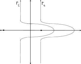
Figure 2: The contours $\tilde{\Gamma}_{\zeta}$ and $\tilde{\Gamma}_{\eta}$ extend vertically along the lines $c_{3}/2$ and $-c_{3}/2$ except for a dimple to the right of $XT^{-1/3}$ so as to avoid the poles of the Gamma function (marked as solid black circles).

its kernel,

$$K_{s}^{\mathrm{edge}}(\tilde{\eta},\tilde{\eta}^{\prime}) = \int_{\tilde{\Gamma}_{\zeta}}\exp\biggl{\{}-\frac{T}{3}(\tilde{\zeta}^{3}-\tilde{\eta}^{\prime 3})+sT^{1/3}(\tilde{\zeta}-\tilde{\eta}^{\prime})\biggr{\}}2^{1/3}$$

$$\hskip 4.0pt\quad{}\times\int_{-\infty}^{\infty}\frac{\tilde{\mu}e^{-2^{1/3}t(\tilde{\zeta}-\tilde{\eta}^{\prime})}}{e^{t}-\tilde{\mu}}\,dt\frac{\Gamma(2^{1/3}\tilde{\zeta}-2^{1/3}XT^{-1/3})}{\Gamma(2^{1/3}\tilde{\eta}^{\prime}-2^{1/3}XT^{-1/3})}\frac{d\tilde{\zeta}}{\tilde{\zeta}-\tilde{\eta}},$$

or, equivalently, evaluating the $t$ integral,

$$K_{s}^{\mathrm{edge}}(\tilde{\eta},\tilde{\eta}^{\prime}) = \int_{\tilde{\Gamma}_{\zeta}}\exp\biggl{\{}-\frac{T}{3}(\tilde{\zeta}^{3}-\tilde{\eta}^{\prime 3})+sT^{1/3}(\tilde{\zeta}-\tilde{\eta}^{\prime})\biggr{\}}$$

$$\hskip 4.0pt\quad{}\times\frac{\pi 2^{1/3}(-\tilde{\mu})^{-2^{1/3}(\tilde{\zeta}-\tilde{\eta}^{\prime})}}{\sin(\pi 2^{1/3}(\tilde{\zeta}-\tilde{\eta}^{\prime}))}\frac{\Gamma(2^{1/3}\tilde{\zeta}-2^{1/3}XT^{-1/3})}{\Gamma(2^{1/3}\tilde{\eta}^{\prime}-2^{1/3}XT^{-1/3})}\frac{d\tilde{\zeta}}{\tilde{\zeta}-\tilde{\eta}}.$$

$\Gamma(z)$ is the standard Gamma function, defined for $\operatorname{Re}(z)>0$ by $\Gamma(z)=\int_{0}^{\infty}s^{z-1}\times e^{-s}\,ds$ and extended by analytic continuation to $\mathbb{C}-\{0,-1,-2,\ldots\}$. To follow previous works we continue to use the letter gamma for contours, but always with a subscript to differentiate them from the Gamma function.

Definition 19.

The fan crossover distribution is defined as

$$F^{\mathrm{fan}}_{T,X}(s)=\int_{\tilde{\mathcal{C}}}e^{-\tilde{\mu}}\frac{d\tilde{\mu}}{\tilde{\mu}}\det(I-K^{\mathrm{fan}}_{s})_{L^{2}(\tilde{\Gamma}_{\eta})}.$$

The kernel $K_{s}^{\mathrm{fan}}$ acts on the function space $L^{2}(\tilde{\Gamma}_{\eta})$ through its kernel,

$$K_{s}^{\mathrm{fan}}(\tilde{\eta},\tilde{\eta}^{\prime}) = \int_{\tilde{\Gamma}_{\zeta}}\exp\biggl{\{}-\frac{T}{3}(\tilde{\zeta}^{3}-\tilde{\eta}^{\prime 3})+sT^{1/3}(\tilde{\zeta}-\tilde{\eta}^{\prime})\biggr{\}}2^{1/3}$$

$$\hskip 4.0pt\quad{}\times\biggl{(}\int_{-\infty}^{\infty}\frac{\tilde{\mu}e^{-2^{1/3}t(\tilde{\zeta}-\tilde{\eta}^{\prime})}}{e^{t}-\tilde{\mu}}\,dt\biggr{)}\frac{d\tilde{\zeta}}{\tilde{\zeta}-\tilde{\eta}},$$

or, evaluating the inner integral, equivalently,

$$K_{s}^{\mathrm{fan}}(\tilde{\eta},\tilde{\eta}^{\prime}) = \int_{\tilde{\Gamma}_{\zeta}}\exp\biggl{\{}-\frac{T}{3}(\tilde{\zeta}^{3}-\tilde{\eta}^{\prime 3})+sT^{1/3}(\tilde{\zeta}-\tilde{\eta}^{\prime})\biggr{\}}$$

$$\quad\hskip 4.0pt{}\times\frac{\pi 2^{1/3}(-\tilde{\mu})^{-2^{1/3}(\tilde{\zeta}-\tilde{\eta}^{\prime})}}{\sin(\pi 2^{1/3}(\tilde{\zeta}-\tilde{\eta}^{\prime}))}\frac{d\tilde{\zeta}}{\tilde{\zeta}-\tilde{\eta}}.$$

As far as the choice of contours $\tilde{\Gamma}_{\zeta}$ and $\tilde{\Gamma}_{\eta}$, one can use the same as above without the extra dimple (since there are no poles to avoid now). This distribution is closely related to the crossover distribution of ACQ , though one observes that the scalings are slightly different. As we now have a whole class of crossover distributions we find it useful to name them more descriptively.

Definition 20.

The Airy₂ process is defined in terms of finite dimensional distributions as

$$P\Biggl{(}\bigcap_{k=1}^{m}\{\mathcal{A}_{2}(X_{k})\leq s_{k}\}\Biggr{)}=\det(I-\chi_{s}K_{\mathcal{A}_{2}}\chi_{s})_{L^{2}(\{X_{1},\ldots,X_{m}\}\times\mathbb{R})},$$

where $\chi_{s}(X_{k},x)=\mathbf{1}_{[x>s_{k}]}$, and $K_{\mathcal{A}_{2}}$ is the extended Airy kernel

$$K_{\mathcal{A}_{2}}(X,x;X^{\prime},y)=\cases{{\displaystyle\int_{0}^{\infty}\,dt\,e^{(X^{\prime}-X)t}\operatorname{Ai}(t+x)\operatorname{Ai}(t+y)},&\quad$X\geq X^{\prime},$\vspace*{2pt}\cr{-\displaystyle\int_{-\infty}^{0}\,dt\,e^{(X^{\prime}-X)t}\operatorname{Ai}(t+x)\operatorname{Ai}(t+y)},&\quad$X<X^{\prime}.$}$$

The Airy₂ process was discovered in the PNG model PS . It is a stationary process with one-point distribution given by the GUE Tracy–Widom distribution $F_{\mathrm{GUE}}$ TW0 . An integral representation of $K_{\mathcal{A}_{2}}$ can be found in Proposition 2.3 of JDTASEP ; another form is in Definition 21 of BFS09 in the $M=0$ case.

We denote by $\mathcal{A}_{2\to\mathrm{BM}}$ the transition process from Airy₂ to Brownian motion. It is defined in terms of finite dimensional distributions as

$$P\Biggl{(}\bigcap_{k=1}^{m}\{\mathcal{A}_{2\to\mathrm{BM}}(X_{k})\leq s_{k}\}\Biggr{)}=\det(I-\chi_{s}K_{\mathcal{A}_{\mathrm{BM}\to 2}}\chi_{s})_{L^{2}(\{X_{1},\ldots,X_{m}\}\times\mathbb{R})},$$

where $K_{\mathcal{A}_{2\to\mathrm{BM}}}$ is the rank-one perturbation $K_{\mathcal{A}_{2}}$,

$$K_{\mathcal{A}_{2\to\mathrm{BM}}}(X,x;X^{\prime},y)$$

$$\qquad=K_{\mathcal{A}_{2}}(X,x;X^{\prime},y)+\operatorname{Ai}(x)\biggl{(}-e^{(1/3)X^{\prime 3}+X^{\prime}y}-\int_{0}^{\infty}\,dt\,\operatorname{Ai}(t+y)e^{-X^{\prime}t}\biggr{)}.$$

This transition process was derived in SI04 and was shown to arise in TASEP at the edge of the rarefaction fan in CFP . An integral representation of the kernel can be found in BFS09 , Definition 21, in the $m=1$ case. For $m=1$ this formula corresponds with the distribution $F_{1}$ of BBP .

The definition of the process for equilibrium TASEP, $\mathcal{A}_{\mathrm{eq}}$, is quite intricate and is given in BFP where it is actually called the $\mathcal{A}_{\mathrm{stat}}$ process. Its joint distributions is the right-hand side of equation (1.9) in BFP .

3 Weakly asymmetric limit of the Tracy–Widom step Bernoulli ASEP formula

In this section we will prove our main result, Theorem 3. The proof of that theorem follows by combining the proof of the main theorem of ACQ (for step initial condition WASEP) with a few lemmas to cover a new element [the $g(\zeta)$ term stated below] which shows up for step Bernoulli initial conditions. As noted in the Introduction, the key technical tool behind this proof is the exact formula for the transition probability of a single particle in ASEP with step Bernoulli initial data TW4 .

Theorem 21 ((Main results of TW4 ))

Let $q>p$ with $q+p=1$, $\gamma=q-p$ and $\tau=p/q$. Fix $\rho_{-}=0$, and for $\rho_{+}\in(0,1]$, set

$$\alpha=(1-\rho_{+})/{\rho_{+}}.$$

Since $\rho_{-}=0$ we can initially label our particles $1,2,3,\ldots$ by setting the leftmost to be particle 1 and the second left most to be particle 2, and so on. Let $\mathbf{x}(t,m)$ denote the location of particle $m$ at time $t$. Then for $m>0$, $t\geq 0$ and $x\in\mathbb{Z}$, TW4 gives the following exact formula:

$$P\bigl{(}\mathbf{x}(\gamma^{-1}t,m)\leq x\bigr{)}=\int_{S_{\tau^{+}}}\frac{d\mu}{\mu}\prod_{k=0}^{\infty}(1-\mu\tau^{k})\det(I+\mu J^{\Gamma}_{\mu})_{L^{2}(\Gamma_{\eta})},$$ (36)

where $S_{\tau^{+}}$ is a circle centered at zero of radius strictly between $\tau$ and 1, and where the kernel of the determinant is given by

$$J^{\Gamma}_{\mu}(\eta,\eta^{\prime})=\int_{\Gamma_{\zeta}}\exp\{\Psi(\zeta)-\Psi(\eta^{\prime})\}\frac{f(\mu,\zeta/\eta^{\prime})}{\eta^{\prime}(\zeta-\eta)}\frac{g(\eta^{\prime})}{g(\zeta)}\,d\zeta,$$ (37)

where

$$f(\mu,z) = \sum_{k=-\infty}^{\infty}\frac{\tau^{k}}{1-\tau^{k}\mu}z^{k},$$

$$\Psi(\zeta) = \Lambda(\zeta)-\Lambda(\xi),$$ (38)

$$\Lambda(\zeta) = -x\log(1-\zeta)+\frac{t\zeta}{1-\zeta}+m\log\zeta,$$

$$g(\zeta) = \prod_{n=0}^{\infty}(1+\tau^{n}\alpha\zeta).$$ (39)

The contours are a little tricky: $\eta$ and $\eta^{\prime}$ are on $\Gamma_{\eta}$, a circle of diameter $[-\alpha^{-1}+2\delta,1-\delta]$ for $\delta$ small. And the $\zeta$ integral is on $\Gamma_{\zeta}$, a circle of diameter $[-\alpha^{-1}+\varsigma,1+\varsigma]$. One should choose $\varsigma$ so as to ensure that $|\zeta/\eta|\in(1,\tau^{-1})$. This choice of contour avoids the poles of the new infinite product which are at $-\alpha^{-1}\tau^{-n}$ for $n\geq 0$. Of course we can take $\delta$ to depend on $\varepsilon$.

3.1 Heuristic explanation of the asymptotics of the Tracy–Widom formula

We start by restating the result and give a heuristic explanation of the proof. In Section 3.2 we will give a complete proof of these asymptotics, roughly following the method of proof of Theorem 1 of ACQ .

The following theorem uses different scalings so as to conform to the notation of ACQ . Therefore, the resulting formula differs and we introduce the kernel $K_{a}^{\csc,\Gamma}$. From the following result, by careful scaling, one arrives at Theorem 3.

Theorem 22 ((Equivalent to Theorem 3 after rescaling))

Consider $\varepsilon>0$, $T>0$ and $X\in\mathbb{R}$ and set $\rho_{-}=0$, $\rho_{+}=1/2$, $t=\varepsilon^{-3/2}T$, $x=\varepsilon^{-1}X$ and $\gamma=\varepsilon^{1/2}$. Then

$$\lim_{\varepsilon\rightarrow 0}P\biggl{(}\varepsilon^{1/2}\biggl{[}h_{\gamma}\biggl{(}\frac{t}{\gamma},x\biggr{)}-\frac{t}{2}\biggr{]}\geq-s\biggr{)} = \lim_{\varepsilon\rightarrow 0}P\biggl{(}\mathbf{x}_{\gamma}\biggl{(}\frac{t}{\gamma},m\biggr{)}\leq x\biggr{)}$$

$$= \int_{\tilde{C}}e^{-\tilde{\mu}}\det(I-K_{a}^{\csc,\Gamma})_{L^{2}(\tilde{\Gamma}_{\eta})}\frac{d\tilde{\mu}}{\tilde{\mu}},$$

where $a=a(s)=s+\frac{X^{2}}{2T}$,

$$m=\frac{1}{2}\biggl{[}\varepsilon^{-1/2}\biggl{(}-a+\frac{X^{2}}{2T}\biggr{)}+\frac{t}{2}+x\biggr{]}$$

and the operator $K_{a}^{\csc,\Gamma}$ acts on the function space $L^{2}(\tilde{\Gamma}_{\eta})$ through its kernel,

$$K_{a}^{\csc,\Gamma}(\tilde{\eta},\tilde{\eta}^{\prime}) = \int_{\tilde{\Gamma}_{\zeta}}\exp\biggl{\{}-\frac{T}{3}(\tilde{\zeta}^{3}-\tilde{\eta}^{\prime 3})+2^{1/3}a(\tilde{\zeta}-\tilde{\eta}^{\prime})\biggr{\}}2^{1/3}$$

$$\quad\hskip 4.0pt{}\times\biggl{(}\int_{-\infty}^{\infty}\frac{\tilde{\mu}e^{-2^{1/3}t(\tilde{\zeta}-\tilde{\eta}^{\prime})}}{e^{t}-\tilde{\mu}}\,dt\biggr{)}\frac{\Gamma(2^{1/3}\tilde{\zeta}-{X}/{T})}{\Gamma(2^{1/3}\tilde{\eta}^{\prime}-{X}/{T})}\frac{d\tilde{\zeta}}{\tilde{\zeta}-\tilde{\eta}}.$$

The contours $\tilde{\mathcal{C}}$, $\tilde{\Gamma}_{\zeta}$ and $\tilde{\Gamma}_{\eta}$ are defined in Definition 18, though for the last two contours, the dimples are modified to go to the right of the poles of the Gamma function above (the rightmost of which lies at $2^{-1/3}X/T$).

We now proceed with the heuristic proof of the above result. Note that given the values of $\rho_{-}$ and $\rho_{+}$, the parameter $\alpha$ defined above in Theorem 21 is equal to 1. We will, however, keep $\alpha$ in the calculations since one can then see readily how to generalize to $\alpha\neq 1$.

The first term in the integrand of (36) is the infinite product $\prod_{k=0}^{\infty}(1-\mu\tau^{k})$. Observe that $\tau=q/p\approx 1-2\varepsilon^{1/2}$ and that $S_{\tau^{+}}$, the contour on which $\mu$ lies, is a circle centered at zero of radius between $\tau$ and 1. The infinite product is not well behaved along most of this contour; however, we can deform the contour to one along which the product is not highly oscillatory. Care must be taken, however, since the Fredholm determinant has poles at every $\mu=\tau^{k}$. The deformation must avoid passing through them. As in ACQ observe that if

$$\mu=\varepsilon^{1/2}\tilde{\mu},$$ (41)

then

$$\prod_{k=0}^{\infty}(1-\mu\tau^{k})\approx e^{-\sum_{k=0}^{\infty}\mu\tau^{k}}=e^{-\mu/(1-\tau)}\approx e^{-\tilde{\mu}/2}.$$

We make the $\mu\mapsto\varepsilon^{-1/2}\tilde{\mu}$ change of variables and find that if we consider a $\tilde{\mu}$ contour

$$\tilde{\mathcal{C}}_{\varepsilon}=\{e^{i\theta}\}_{\pi/2\leq\theta\leq 3\pi/2}\cup\{x\pm i\}_{0<x\leq\varepsilon^{-1/2}-1}\cup\{\varepsilon^{-1/2}-1+iy\}_{-1<y<1},$$

then the above approximations are reasonable. Thus the infinite product goes to $\exp\{-\tilde{\mu}/2\}$.

Now we turn to the Fredholm determinant and determine a candidate for the pointwise limit of the kernel. The kernel $J^{\Gamma}_{\mu}(\eta,\eta^{\prime})$ is given by an integral whose integrand has four main components: an exponential

$$\exp\{\Lambda(\zeta)-\Lambda(\eta^{\prime})\};$$

a rational function (we include the differential with this term for scaling purposes)

$${d\zeta}/{\eta^{\prime}(\zeta-\eta)};$$

a doubly infinite sum

$$\mu f(\mu,\zeta/\eta^{\prime});$$

an infinite product

$${g(\eta^{\prime})}/{g(\zeta)}.$$

We proceed by the method of steepest descent, so in order to determine the region along the $\zeta$ and $\eta$ contours which affects the asymptotics, we must consider the exponential term first. The argument of the exponential is given by $\Lambda(\zeta)-\Lambda(\eta^{\prime})$ where

$$\Lambda(\zeta)=-x\log(1-\zeta)+\frac{t\zeta}{1-\zeta}+m\log(\zeta),$$

where $x$, $t$ and $m$ are as in Theorem 22. For small $\varepsilon$, $\Lambda(\zeta)$ has a critical point in an $\varepsilon^{1/2}$ neighborhood of $-1$. For purposes of having a nice ultimate answer, we choose to center in on the point

$$\xi=-1-2\varepsilon^{1/2}\frac{X}{T}.$$

We can rewrite the argument of the exponential as $(\Lambda(\zeta)-\Lambda(\xi))-(\Lambda(\eta^{\prime})-\Lambda(\xi))=\Psi(\zeta)-\Psi(\eta^{\prime})$. The idea of extracting asymptotics for this term (which starts like those done in TW3 but quickly becomes more involved due to the fact that $\tau$ tends to 1 as $\varepsilon$ goes to zero) is then to deform the $\zeta$ and $\eta$ contours to lie along curves such that outside the scale $\varepsilon^{1/2}$ around $\xi$, $\operatorname{Re}\Psi(\zeta)$ is very negative, and $\operatorname{Re}\Psi(\eta^{\prime})$ is very positive, and hence the contribution from those parts of the contours is negligible. Rescaling around $\xi$ to blow up this $\varepsilon^{1/2}$ scale, gives us the asymptotic exponential term. This change of variables sets the scale at which we should analyze the other three terms in the integrand for the $J$ kernel.

Returning to $\Psi(\zeta)$, we make a Taylor expansion around $\xi$ and find that in a neighborhood of $\xi$,

$$\Psi(\zeta)\approx-\frac{T}{48}\varepsilon^{-3/2}(\zeta-\xi)^{3}+\frac{a}{2}\varepsilon^{-1/2}(\zeta-\xi).$$

This suggests the following change of variables:

$$\tilde{\zeta} = 2^{-4/3}\varepsilon^{-1/2}(\zeta-\xi),\qquad\tilde{\eta}=2^{-4/3}\varepsilon^{-1/2}(\eta-\xi),$$

$$\tilde{\eta}^{\prime} = 2^{-4/3}\varepsilon^{-1/2}(\eta^{\prime}-\xi),$$

after which our Taylor expansion takes the form

$$\Psi(\tilde{\zeta})\approx-\frac{T}{3}\tilde{\zeta}^{3}+2^{1/3}a\tilde{\zeta}.$$

In the spirit of steepest descent analysis we would like the $\zeta$ contour to leave $\xi$ in a direction where this Taylor expansion is decreasing rapidly. This is accomplished by leaving at an angle $\pm 2\pi/3$. Likewise, since $\Psi(\eta)$ should increase rapidly, $\eta$ should leave $\xi$ at angle $\pm\pi/3$. Since $\rho_{+}=1/2$, $\alpha=1$ which means that the $\zeta$ contour is originally on a circle of diameter $[-1+\delta,1+\delta]$ and the $\eta$ contour on a circle of diameter $[-1+2\delta,1-\delta]$ for some positive $\delta$ [which can and should depend on $\varepsilon$ so as to ensure that $|\zeta/\eta|\in(1,\tau^{-1})$]. In order to deform these contours to their steepest descent contours without changing the value of the determinant, great care must be taken to avoid the poles of $f$, which occur whenever $\zeta/\eta^{\prime}=\tau^{k}$, $k\in\mathbb{Z}$, and the poles of $1/g$, which occur whenever $\zeta=-\tau^{-n}$, $n\geq 0$. We will ignore these considerations in the formal calculation but will take them up more carefully in Section 3.2. The one very important consideration in this deformation, even formally, is that we must end up with contours which lie to the right of the poles of the $1/g$ function.

Let us now assume that we can deform our contours to curves along which $\Psi$ rapidly decays in $\zeta$ and increases in $\eta$, as we move along them away from $\xi$. If we apply the change of variables in (3.1) the straight part of our contours become infinite rays at angles $\pm 2\pi/3$ and $\pm\pi/3$ which we call $\tilde{\Gamma}_{\zeta}$ and $\tilde{\Gamma}_{\eta}$. Note that this is not the actual definition of these contours which we use in the statement and proof of Theorem 3 because of the singularity problem mentioned above.

Applying this change of variables to the kernel of the Fredholm determinant changes the $L^{2}$ space, and hence we must multiply the kernel by the Jacobian term $2^{4/3}\varepsilon^{1/2}$. We will include this term with the $\mu f(\mu,z)$ term and take the $\varepsilon\to 0$ limit of that product.

Before we consider that term, however, it is worth looking at the new infinite product term $g(\eta^{\prime})/g(\zeta^{\prime})$. In order to do that let us consider the following. Set

$$q=1-r,\qquad a=\frac{\log\alpha(c-xr)}{\log q},\qquad b=\frac{\log\alpha(c-yr)}{\log q}.$$

Then observe that

$$\prod_{n=0}^{\infty}\frac{1+(1-r)^{n}\alpha(-c+xr)}{1+(1-r)^{n}\alpha(-c+yr)}$$

$$\qquad=\frac{(q^{a};q)_{\infty}}{(q^{b};q)_{\infty}}=\frac{\Gamma_{q}(b)}{\Gamma_{q}(a)}(1-q)^{b-a}=\frac{\Gamma_{q}(b)}{\Gamma_{q}(a)}e^{(b-a)\log r}$$ (43)

$$\qquad=\frac{\Gamma_{1-r}(-r^{-1}\log(\alpha c)+c^{-1}y+o(r))}{\Gamma_{1-r}(-r^{-1}\log(\alpha c)+c^{-1}x+o(r))}e^{c^{-1}(y-x)\log r+o(r\log r)},$$

where the $q$-Gamma function and the $q$-Pochhammer symbols are given by

$$\Gamma_{q}(x):=\frac{(q;q)_{\infty}}{(q^{x};q)_{\infty}}(1-q)^{1-x}$$

when $|q|<1$ and

$$(a;q)_{\infty}=(1-a)(1-aq)(1-aq^{2})\cdots.$$

The notation $o(f(r))$ above refers to a function $f^{\prime}(r)$ such that $f^{\prime}(r)/f(r)\to 0$ as $r\to 0$. The $q$-Gamma function converges to the usual Gamma function as $q\to 1$, uniformly on compact sets; see AAR for more details and a statement of this result.

Now consider the $g$ terms and observe that in the rescaled variables this corresponds with (3.1) with $r=2\varepsilon^{1/2}$, $c=1$ (recall $\alpha=1$ as well) and

$$y=2^{1/3}\tilde{\zeta}-\frac{X}{T},\qquad x=2^{1/3}\tilde{\eta}^{\prime}-\frac{X}{T}.$$

Since $\alpha c=1$ and since we are away from the poles and zeros of the Gamma functions, we find that

$$\frac{g(\eta^{\prime})}{g(\zeta)}\rightarrow\frac{\Gamma(2^{1/3}\tilde{\zeta}-{X}/{T})}{\Gamma(2^{1/3}\tilde{\eta}^{\prime}-{X}/{T})}\exp\{2^{1/3}(\tilde{\zeta}-\tilde{\eta}^{\prime})\log(2\varepsilon^{1/2})\}.$$ (44)

This exponential can be rewritten as

$$\exp\biggl{\{}\frac{\tilde{z}}{4}\log\varepsilon\biggr{\}}\exp\{2^{1/3}\log(2)(\tilde{\zeta}-\tilde{\eta}^{\prime})\},$$ (45)

where

$$\tilde{z}=2^{4/3}(\tilde{\zeta}-\tilde{\eta}^{\prime}).$$ (46)

It appears that there is a problem in these asymptotics as $\varepsilon$ goes to zero; however, we will find that this apparent divergence exactly cancels with a similar term in the doubly infinite summation term asymptotics. We will now show how that $\log\varepsilon$ in the exponent can be absorbed into the $2^{4/3}\varepsilon^{1/2}\mu f(\mu,\zeta/\eta^{\prime})$ term. Recall

$$\mu f(\mu,z)=\sum_{k=-\infty}^{\infty}\frac{\mu\tau^{k}}{1-\tau^{k}\mu}z^{k}.$$

If we let $n_{0}=\lfloor\log(\varepsilon^{-1/2})/\log(\tau)\rfloor$, then observe that

$$\mu f(\mu,z)=\sum_{k=-\infty}^{\infty}\frac{\mu\tau^{k+n_{0}}}{1-\tau^{k+n_{0}}\mu}z^{k+n_{0}}=z^{n_{0}}\tau^{n_{0}}\mu\sum_{k=-\infty}^{\infty}\frac{\tau^{k}}{1-\tau^{k}\tau^{n_{0}}\mu}z^{k}.$$

By the choice of $n_{0}$, $\tau^{n_{0}}\approx\varepsilon^{-1/2}$, so

$$\mu f(\mu,z)\approx z^{n_{0}}\tilde{\mu}f(\tilde{\mu},z).$$

The discussion on the exponential term indicates that it suffices to understand the behavior of this function only in the region where $\zeta$ and $\eta^{\prime}$ are within a neighborhood of $\xi$ of order $\varepsilon^{1/2}$. Equivalently, letting $z=\zeta/\eta^{\prime}$, it suffices to understand $\mu f(\mu,z)\approx z^{n_{0}}\tilde{\mu}f(\tilde{\mu},z)$ for

$$z=\frac{\zeta}{\eta^{\prime}}=\frac{\xi+2^{4/3}\varepsilon^{1/2}\tilde{\zeta}}{\xi+2^{4/3}\varepsilon^{1/2}\tilde{\eta}^{\prime}}\approx 1-\varepsilon^{1/2}\tilde{z}.$$

Let us now consider $z^{n_{0}}$ using the fact that $\log\tau\approx-2\varepsilon^{1/2}$.

$$z^{n_{0}}\approx(1-\varepsilon^{1/2}\tilde{z})^{\varepsilon^{-1/2}({1}/{4})\log\varepsilon}\approx e^{-({1}/{4})\tilde{z}\log\varepsilon}.$$

Plugging back in the value of $\tilde{z}$ in terms of $\tilde{\zeta}$ and $\tilde{\eta}^{\prime}$ we see that this prefactor of $z^{n_{0}}$ exactly cancels the $\log\varepsilon$ term which came from the $g$ infinite product term.

What remains is to determine the limit of $2^{4/3}\varepsilon^{1/2}\tilde{\mu}f(\tilde{\mu},z)$ as $\varepsilon$ goes to zero and for $z\approx 1-\varepsilon^{1/2}\tilde{z}$. This limit can be found by interpreting the infinite sum as a Riemann sum approximation for an appropriate integral. Define $t=k\varepsilon^{1/2}$, then observe that

$$\varepsilon^{1/2}\tilde{\mu}f(\tilde{\mu},z)=\sum_{k=-\infty}^{\infty}\frac{\tilde{\mu}\tau^{t\varepsilon^{-1/2}}z^{t\varepsilon^{-1/2}}}{1-\tilde{\mu}\tau^{t\varepsilon^{-1/2}}}\varepsilon^{1/2}\rightarrow\int_{-\infty}^{\infty}\frac{\tilde{\mu}e^{-2t}e^{-\tilde{z}t}}{1-\tilde{\mu}e^{-2t}}\,dt.$$

This used the fact that $\tau^{t\varepsilon^{-1/2}}\rightarrow e^{-2t}$ and that $z^{t\varepsilon^{-1/2}}\rightarrow e^{-\tilde{z}t}$, which hold at least pointwise in $t$. If we change variables of $t$ to $t/2$ and multiply the top and bottom by $e^{-t}$, then we find that

$$2^{4/3}\varepsilon^{1/2}\mu f(\mu,\zeta/\eta^{\prime})\rightarrow 2^{1/3}\int_{-\infty}^{\infty}\frac{\tilde{\mu}e^{-\tilde{z}t/2}}{e^{t}-\tilde{\mu}}\,dt.$$

As far as the final term, the rational expression, under the change of variables and zooming in on $\xi$, the factor of $1/\eta^{\prime}$ goes to $-1$ and the $\frac{d\zeta}{\zeta-\eta^{\prime}}$ goes to $\frac{d\tilde{\zeta}}{\tilde{\zeta}-\tilde{\eta}^{\prime}}$.

Therefore we formally find the following kernel: $-K_{a^{\prime}}^{\csc,\Gamma}(\tilde{\eta},\tilde{\eta}^{\prime})$ acting on $L^{2}(\tilde{\Gamma}_{\eta})$, where

$$K_{a^{\prime}}^{\csc,\Gamma}(\tilde{\eta},\tilde{\eta}^{\prime}) = \int_{\tilde{\Gamma}_{\zeta}}\exp\biggl{\{}-\frac{T}{3}(\tilde{\zeta}^{3}-\tilde{\eta}^{\prime 3})+2^{1/3}a^{\prime}(\tilde{\zeta}-\tilde{\eta}^{\prime})\biggr{\}}2^{1/3}$$

$$\quad\hskip 4.0pt{}\times\biggl{(}\int_{-\infty}^{\infty}\frac{\tilde{\mu}e^{-2^{1/3}t(\tilde{\zeta}-\tilde{\eta}^{\prime})}}{e^{t}-\tilde{\mu}}\,dt\biggr{)}\frac{\Gamma(2^{1/3}\tilde{\zeta}-{X}/{T})}{\Gamma(2^{1/3}\tilde{\eta}^{\prime}-{X}/{T})}\frac{d\tilde{\zeta}}{\tilde{\zeta}-\tilde{\eta}},$$

where $a^{\prime}=a+\log 2$ [recall that this $\log 2$ came from (45)].

We have the identity

$$\int_{-\infty}^{\infty}\frac{\tilde{\mu}e^{-\tilde{z}t/2}}{e^{t}-\tilde{\mu}}\,dt=(-\tilde{\mu})^{-\tilde{z}/2}\pi\csc(\pi\tilde{z}/2),$$ (47)

where the branch cut in $\tilde{\mu}$ is along the positive real axis, hence $(-\tilde{\mu})^{-\tilde{z}/2}=e^{-\log(-\tilde{\mu})\tilde{z}/2}$ where $\log$ is taken with the standard branch cut along the negative real axis. We may use the identity to rewrite the kernel as

$$K_{a^{\prime}}^{\csc,\Gamma}(\tilde{\eta},\tilde{\eta}^{\prime}) = \int_{\tilde{\Gamma}_{\zeta}}\exp\biggl{\{}-\frac{T}{3}(\tilde{\zeta}^{3}-\tilde{\eta}^{\prime 3})+2^{1/3}a^{\prime}(\tilde{\zeta}-\tilde{\eta}^{\prime})\biggr{\}}2^{1/3}$$

$$\hskip 4.0pt\quad{}\times\frac{\pi(-\tilde{\mu})^{-2^{1/3}(\tilde{\zeta}-\tilde{\eta}^{\prime})}}{\sin(\pi 2^{1/3}(\tilde{\zeta}-\tilde{\eta}^{\prime}))}\frac{\Gamma(2^{1/3}\tilde{\zeta}-{X}/{T})}{\Gamma(2^{1/3}\tilde{\eta}^{\prime}-{X}/{T})}\frac{d\tilde{\zeta}}{\tilde{\zeta}-\tilde{\eta}}.$$

To make this cleaner we replace $\tilde{\mu}/2$ with $\tilde{\mu}$. Taking into account this change of variables (it also changes the $\exp\{-\tilde{\mu}/2\}$ in front of the determinant to $\exp\{-\tilde{\mu}\}$), we find that our final answer is

$$\int_{\tilde{\mathcal{C}}}e^{-\tilde{\mu}}\frac{d\tilde{\mu}}{\tilde{\mu}}\det(I-K_{a}^{\csc,\Gamma})_{L^{2}(\tilde{\Gamma}_{\eta})},$$

which, up to the definitions of the contours $\tilde{\Gamma}_{\eta}$ and $\tilde{\Gamma}_{\zeta}$, is the desired limiting formula.

It is important to note the many possible pitfalls of such a heuristic computation: (1) Pointwise convergence of both the prefactor infinite product and the Fredholm determinant is not enough to prove convergence of the $\tilde{\mu}$ integral; (2) the deformations of the $\eta$ and $\zeta$ contours to the steepest descent curves are invalid, as they pass through multiple poles of the kernel, coming both from the $f$ term and the $g$ term; (3) one has to show that the kernels converge in the sense of trace norm as opposed to just pointwise. The Riemann sum approximation argument can in fact be made rigorous though; in ACQ an alternative proof of the validity of that limit is given via analysis of singularities and residues.

These possible pitfalls are addressed below in Section 3.2.

3.2 Proof of Theorem 3

In this section we provide a complete proof of Theorem 22, from which one recovers Theorem 3 via scaling. The proof follows the same argument to that of ACQ . As a convention, $c$ (or capitalized, primed, etc., versions) will represent a finite constant which can vary line to line, unless explicitly noted.

In Theorem 22, we have reformulated the claim of Theorem 3 in terms of the weakly asymmetric simple exclusion process with half step Bernoulli initial data. Our proof, therefore, reduces to a rigorous asymptotic analysis of Tracy and Widom’s formula (36). That formula contains an integral over a $\mu$ contour of a product of a prefactor infinite product and a Fredholm determinant. The first step toward taking the limit of this as $\varepsilon$ goes to zero is to control the prefactor, $\prod_{k=0}^{\infty}(1-\mu\tau^{k})$. Initially $\mu$ lies on a contour $S_{\tau^{+}}$ which is centered at zero and of radius between $\tau$ and 1. Along this contour the partial products (i.e., product up to $N$) form a highly oscillatory sequence, and hence it is hard to control the convergence of the sequence.

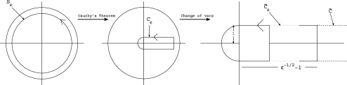
Figure 3: The $S_{\varepsilon}$ contour is deformed to the $C_{\varepsilon}$ contour via Cauchy’s theorem, and then a change of variables leads to $\tilde{C}_{\varepsilon}$, with its infinite extension $\tilde{C}$.

The first step in our proof is to deform the $\mu$ contour $S_{\tau^{+}}$ to the long, skinny cigar-shaped contour

$$\mathcal{C}_{\varepsilon}=\{\varepsilon^{1/2}e^{i\theta}\}_{\pi/2\leq\theta\leq 3\pi/2}\cup\{x\pm i\varepsilon^{1/2}\}_{0<x\leq 1-\varepsilon^{1/2}}\cup\{1-\varepsilon^{1/2}+\varepsilon^{1/2}iy\}_{-1<y<1};$$

see Figure 3. We orient $\mathcal{C}_{\varepsilon}$ counter-clockwise. Notice that this new contour still includes all of the poles at $\mu=\tau^{k}$ associated with the $f$ function in the $J$ kernel.

In order to justify replacing $S_{\tau^{+}}$ by $\mathcal{C}_{\varepsilon}$ we need the following:

Lemma 23

In equation (36) we can replace the contour $S_{\varepsilon}$ with $\mathcal{C}_{\varepsilon}$ as the contour of integration for $\mu$ without affecting the value of the integral.

We thank the referee for pointing out a mistake in the proof of this result in ACQ , and suggesting an alternative proof which we detail in Section 3.4.2.

Having made this deformation of the $\mu$ contour, we now observe that the natural scale for $\mu$ is on order $\varepsilon^{1/2}$. With this in mind we make the change of variables

$$\mu=\varepsilon^{1/2}\tilde{\mu}.$$

Remark 24.

Throughout the proof of this theorem and its lemmas and propositions, we will use the tilde to denote variables which are $\varepsilon^{1/2}$ rescaled versions of the original, untilded variables.

The $\tilde{\mu}$ variable now lives on the contour

$$\tilde{\mathcal{C}}_{\varepsilon}=\{e^{i\theta}\}_{\pi/2\leq\theta\leq 3\pi/2}\cup\{x\pm i\}_{0<x\leq\varepsilon^{-1/2}-1}\cup\{\varepsilon^{-1/2}-1+iy\}_{-1<y<1},$$

which grow and ultimately approach

$$\tilde{\mathcal{C}}=\{e^{i\theta}\}_{\pi/2\leq\theta\leq 3\pi/2}\cup\{x\pm i\}_{x>0}.$$

In order to show convergence of the integral as $\varepsilon$ goes to zero, we must consider two things, the convergence of the integrand for $\tilde{\mu}$ in some compact region around the origin on $\mathcal{\tilde{C}}$, and the controlled decay of the integrand on $\tilde{\mathcal{C}}_{\varepsilon}$ outside of that compact region. This second consideration will allow us to approximate the integral by a finite integral in $\tilde{\mu}$, while the first consideration will tell us what the limit of that integral is. When all is said and done, we will paste back in the remaining part of the $\tilde{\mu}$ integral and have our answer. With this in mind we give the following bound which is taken word for word from Lemma 2.3 of ACQ and whose proof (given therein) relies only on elementary inequalities for the logarithm.

Lemma 25

Define two regions, depending on a fixed parameter $r\geq 1$,

$$R_{1} = \biggl{\{}\tilde{\mu}\dvtx|\tilde{\mu}|\leq\frac{r}{\sin(\pi/10)}\biggr{\}},$$

$$R_{2} = \biggl{\{}\tilde{\mu}\dvtx\operatorname{Re}(\tilde{\mu})\in\biggl{[}\frac{r}{\tan(\pi/10)},\varepsilon^{-1/2}\biggr{]}\mbox{ and }\operatorname{Im}(\tilde{\mu})\in[-2,2]\biggr{\}}.$$

$R_{1}$ is compact, and $R_{1}\cup R_{2}$ contains all of the contour $\mathcal{\tilde{C}}_{\varepsilon}$. Furthermore define the function (the infinite product after the change of variables)

$$p_{\varepsilon}(\tilde{\mu})=\prod_{k=0}^{\infty}(1-\varepsilon^{1/2}\tilde{\mu}\tau^{k}).$$

Then uniformly in $\tilde{\mu}\in R_{1}$,

$$p_{\varepsilon}(\mu)\to e^{-\tilde{\mu}/2}.$$ (49)

Also, for all $\varepsilon<\varepsilon_{0}$ (some positive constant) there exists a constant $c$, such that for all $\tilde{\mu}\in R_{2}$, we have the following tail bound:

$$|p_{\varepsilon}(\tilde{\mu})|\leq|e^{-\tilde{\mu}/2}||e^{-c\varepsilon^{1/2}\tilde{\mu}^{2}}|.$$ (50)

[By the choice of $R_{2}$, for all $\tilde{\mu}\in R_{2}$, $\operatorname{Re}(\tilde{\mu}^{2})>\delta>0$ for some fixed $\delta$. The constant $c$ can be taken to be $1/8$.]

We now turn our attention to the Fredholm determinant term in the integrand. Just as we did for the prefactor infinite product in Lemma 25 we must establish uniform convergence of the determinant for $\tilde{\mu}$ in a fixed compact region around the origin, and a suitable tail estimate valid outside that compact region. The tail estimate must be such that for each finite $\varepsilon$, we can combine the two tail estimates (from the prefactor and from the determinant) and show that their integral over the tail part of $\tilde{\mathcal{C}}_{\varepsilon}$ is small and goes to zero as we enlarge the original compact region. For this we have the following two propositions (the first is the most substantial and is proved in Section 3.3, while the second is proved in Section 3.4.2).

Proposition 26

Fix $s\in\mathbb{R}$, $T>0$ and $X\in\mathbb{R}$. Then for any compact subset of $\tilde{\mathcal{C}}$, we have that for all $\delta>0$, there exists an $\varepsilon_{0}>0$ such that for all $\varepsilon<\varepsilon_{0}$ and all $\tilde{\mu}$ in the compact subset,

$$\bigl{|}\det(I+\varepsilon^{1/2}\tilde{\mu}J^{\Gamma}_{\varepsilon^{1/2}\tilde{\mu}})_{L^{2}(\Gamma_{\eta})}-\det(I-K^{\csc,\Gamma}_{a^{\prime}})_{L^{2}(\tilde{\Gamma}_{\eta})}\bigr{|}<\delta.$$

Here $a^{\prime}=a+\log 2$ and $K_{a^{\prime},\Gamma}^{\csc}$ is defined in equation (22) and depends implicitly on $\tilde{\mu}$.

Proposition 27

There exist $c,c^{\prime}>0$ and $\varepsilon_{0}>0$ such that for all $\varepsilon<\varepsilon_{0}$ and all $\tilde{\mu}\in\tilde{\mathcal{C}}_{\varepsilon}$,

$$\bigl{|}p_{\varepsilon}(\tilde{\mu})\det(I+\varepsilon^{1/2}\tilde{\mu}J^{\Gamma}_{\varepsilon^{1/2}\tilde{\mu}})_{L^{2}(\Gamma_{\eta})}\bigr{|}\leq c^{\prime}e^{-c|\tilde{\mu}|}.$$

This exponential decay bound on the integrand shows that, by choosing a suitably large (fixed) compact region around zero along the contour $\tilde{\mathcal{C}}_{\varepsilon}$, it is possible to make the $\tilde{\mu}$ integral outside of this region arbitrarily small, uniformly in $\varepsilon\in(0,\varepsilon_{0})$. This means that we may assume henceforth that $\tilde{\mu}$ lies in a compact subset of $\tilde{\mathcal{C}}$.

Now that we are on a fixed compact set of $\tilde{\mu}$, the first part of Lemma 25 and Proposition 26 combine to show that the integrand converges uniformly to

$$\frac{e^{-\tilde{\mu}/2}}{\tilde{\mu}}\det(I-K^{\csc,\Gamma}_{a^{\prime}})_{L^{2}(\tilde{\Gamma}_{\eta}),}$$

and hence the integral converges to the integral with this integrand.

To finish the proof of the limit in Theorem 22, it is necessary that for any $\delta$ we can find a suitably small $\varepsilon_{0}$ such that the difference between the two sides of the limit differ by less than $\delta$ for all $\varepsilon<\varepsilon_{0}$. Technically we are in the position of a $\delta/3$ argument. One portion of $\delta/3$ goes to the cost of cutting off the $\tilde{\mu}$ contour outside of some compact set. Another $\delta/3$ goes to the uniform convergence of the integrand. The final portion goes to repairing the $\tilde{\mu}$ contour. As $\delta$ gets smaller, the cut for the $\tilde{\mu}$ contour must occur further out. Therefore the limiting integral will be over the limit of the $\tilde{\mu}$ contours, which we called $\tilde{\mathcal{C}}$. The final $\delta/3$ is spent on the following proposition, whose proof is given in Section 3.4.2.

Proposition 28

There exists $c,c^{\prime}>0$ such that for all $\tilde{\mu}\in\tilde{\mathcal{C}}$ with $|\tilde{\mu}|\geq 1$,

$$\biggl{|}\frac{e^{-\tilde{\mu}/2}}{\tilde{\mu}}\det(I-K^{\csc,\Gamma}_{a})_{L^{2}(\tilde{\Gamma}_{\eta})}\biggr{|}\leq|c^{\prime}e^{-c\tilde{\mu}}|.$$

Recall that the kernel $K^{\csc,\Gamma}_{a}$ is a function of $\tilde{\mu}$. The argument used to prove this proposition immediately shows that $K_{a}^{\csc,\Gamma}$ is a trace class operator on $L^{2}(\tilde{\Gamma}_{\eta})$.

It is an immediate corollary of this exponential tail bound that for sufficiently large compact sets of $\tilde{\mu}$, the cost to include the rest of the $\tilde{\mu}$ contour is less than $\delta/3$. This, along with the change of variables in $\tilde{\mu}$ described at the end of Section 3.1 finishes the proof of Theorem 22.

3.3 Proof of Proposition 26

In this section we provide all of the steps necessary to prove Proposition 26. To ease understanding of the argument we relegate more technical points to lemmas whose proof we delay to Section 3.4.3.

During the proof of this proposition, it is important to keep in mind that we are assuming that $\tilde{\mu}$ lies in a fixed compact subset of $\tilde{\mathcal{C}}$. Recall that $\tilde{\mu}=\varepsilon^{-1/2}\mu$. We proceed via the following strategy to find the limit of the Fredholm determinant as $\varepsilon$ goes to zero. The first step is to deform the contours $\Gamma_{\eta}$ and $\Gamma_{\zeta}$ to suitable curves along which there exists a small region outside of which the kernel of our operator is exponentially small. This justifies cutting the contours off outside of this small region. We may then rescale everything so this small region becomes order one in size. Then we show uniform convergence of the kernel to the limiting kernel on the compact subset. Finally we need to show that we can complete the finite contour on which this limiting object is defined to an infinite contour without significantly changing the value of the determinant.

Recall from Theorem 21 that $\Gamma_{\zeta}$ is defined to be a circle of diameter $[-1+\varsigma,1+\varsigma]$, while $\Gamma_{\eta}$ is a circle of diameter $[-1+2\varsigma,1-\varsigma]$. The condition imposed on $\varsigma$ is that for $\zeta$ and $\eta$ on the above contours, $|\zeta/\eta|\leq(1,\tau^{-1})$. We take $\varsigma=\varepsilon^{1/2}/2$, and since $\tau^{-1}\approx 1+2\varepsilon^{1/2}$, it is clear that for this choice of $\varsigma$, $|\zeta/\eta|\leq(1,\tau^{-1})$. The choice of contours is also such that the poles of the infinite product $1/g(\zeta)$, which occur at $-\tau^{-n}$ for $n\geq 0$, lie to the left of the contours. Also recall

$$\xi=-1-2\varepsilon^{1/2}\frac{X}{T}.$$

The function $f(\mu,\zeta/\eta^{\prime})$ which shows up in the definition of the kernel for $J$ has poles as every point $\zeta/\eta^{\prime}=z=\tau^{k}$ for $k\in\mathbb{Z}$.

As long as we simultaneously deform the $\Gamma_{\zeta}$ contour as we deform $\Gamma_{\eta}$ so as to keep $\zeta/\eta^{\prime}$ away from these poles, we may use Proposition 42 (Proposition 1 of TW3 ), to justify the fact that the determinant does not change under this deformation. In this way we may deform our contours to the following modified contours $\Gamma_{\eta,l},\Gamma_{\zeta,l}$:

Definition 29.

Let $\Gamma_{\eta,l}$ and $\Gamma_{\zeta,l}$ be two families (indexed by $l>0$) of simple closed contours in $\mathbb{C}$ defined as follows. Let

$$\kappa(\theta)=\frac{2X}{T}\tan^{2}\biggl{(}\frac{\theta}{2}\biggr{)}\log\biggl{(}\frac{2}{1-\cos\theta}\biggr{)}.$$ (51)

Both $\Gamma_{\eta,l}$ and $\Gamma_{\zeta,l}$ will be symmetric across the real axis, so we need only define them on the top half. $\Gamma_{\eta,l}$ begins on the real axis $-1+\varepsilon^{1/2}$ and follows a smooth, northwesterly pointing curve and joins the vertical line with real part $\xi+\varepsilon^{1/2}/2$ (see Figure 2 for an illustration of such a curve). It then follows the straight vertical line for a distance $l\varepsilon^{1/2}$ and then joins the curve

$$\bigl{[}1+\varepsilon^{1/2}\bigl{(}\kappa(\theta)+\alpha\bigr{)}\bigr{]}e^{i\theta}$$ (52)

parametrized by $\theta$ from $\pi-l\varepsilon^{1/2}+O(\varepsilon)$ to $0$, and where $\alpha=-1/2+O(\varepsilon^{1/2})$. The small errors are necessary to make sure that the curves join up at the end of the vertical section of the curve. We extend this to a closed contour by reflection through the real axis and orient it clockwise. We denote the first two parts (the northwesterly pointing curve and vertical line), of the contour by $\Gamma_{\eta,l}^{\mathrm{vert}}$ and the remaining, roughly circular part by $\Gamma_{\eta,l}^{\mathrm{circ}}$. This means that $\Gamma_{\eta,l}=\Gamma_{\eta,l}^{\mathrm{vert}}\cup\Gamma_{\eta,l}^{\mathrm{circ}}$, and along this contour we can think of parametrizing $\eta$ by $\theta\in[0,\pi]$.

We define $\Gamma_{\zeta,l}$ similarly, except that it starts out at $-1+\varepsilon^{1/2}/2$, joins the vertical line with real part $\xi-\varepsilon^{1/2}/2$ and finally joins the curve given by equation (52) where the value of $\theta$ ranges from $\theta=\pi-l\varepsilon^{1/2}+O(\varepsilon)$ to $\theta=0$ and where $\alpha=1/2+O(\varepsilon^{1/2})$. We similarly denote this contour by the union of $\Gamma_{\zeta,l}^{\mathrm{vert}}$ and $\Gamma_{\zeta,l}^{\mathrm{circ}}$.

By virtue of these definitions, it is clear that $\varepsilon^{-1/2}|\zeta/\eta^{\prime}-\tau^{k}|$ stays bounded away from zero for all $k$, that $|\zeta/\eta^{\prime}|$ is bounded in an closed set contained in $(1,\tau^{-1})$ for all $\zeta\in\Gamma_{\zeta,l}$ and $\eta\in\Gamma_{\eta,l}$ and that $\varepsilon^{1/2}(\zeta+1)$ is bounded from zero. Therefore, for any $l>0$ we may, by deforming both the $\eta$ and $\zeta$ contours simultaneously, assume that our operator acts on $L^{2}(\Gamma_{\eta,l})$ and that its kernel is defined via an integral along $\Gamma_{\zeta,l}$. It is critical that we now show that, due to our choice of contours, we are able to forget about everything except for the northwesterly pointing curve and vertical part of the contours. To formulate this we have the following:

Definition 30.

Let $\chi_{l}^{\mathrm{vert}}$ and $\chi_{l}^{\mathrm{circ}}$ be projection operators acting on $L^{2}(\Gamma_{\eta,l})$ which project onto $L^{2}(\Gamma_{\eta,l}^{\mathrm{vert}})$ and $L^{2}(\Gamma_{\eta,l}^{\mathrm{circ}})$, respectively. Also define two operators $J_{l}^{\mathrm{vert},\Gamma}$ and $J_{l}^{\mathrm{circ},\Gamma}$ which act on $L^{2}(\Gamma_{\eta,l})$ and have kernels identical to $J^{\Gamma}$ [see equation (37)], except the $\zeta$ integral is over $\Gamma_{\zeta,l}^{\mathrm{vert}}$ and $\Gamma_{\zeta,l}^{\mathrm{circ}}$, respectively. Thus we have a family (indexed by $l>0$) of decompositions of our operator $J$ as follows:

$$J^{\Gamma}=J_{l}^{\mathrm{vert},\Gamma}\chi_{l}^{\mathrm{vert}}+J_{l}^{\mathrm{vert},\Gamma}\chi_{l}^{\mathrm{circ}}+J_{l}^{\mathrm{circ},\Gamma}\chi_{l}^{\mathrm{vert}}+J_{l}^{\mathrm{circ},\Gamma}\chi_{l}^{\mathrm{circ}}.$$

We now show that it suffices to just consider the first part of this decomposition ($J_{l}^{\mathrm{vert},\Gamma}\chi_{l}^{\mathrm{vert}}$) for sufficiently large $l$.

Proposition 31

Assume that $\tilde{\mu}$ is restricted to a bounded subset of the contour $\tilde{\mathcal{C}}$. For all $\delta>0$ there exist $\varepsilon_{0}>0$ and $l_{0}>0$ such that for all $\varepsilon<\varepsilon_{0}$ and all $l>l_{0}$,

$$\bigl{|}\det(I+\mu J^{\Gamma}_{\mu})_{L^{2}(\Gamma_{\eta,l})}-\det(I+J_{l}^{\mathrm{vert},\Gamma})_{L^{2}(\Gamma_{\eta,l}^{\mathrm{vert}})}\bigr{|}<\delta.$$

As was explained in the Introduction, if we let

$$n_{0}=\lfloor\log(\varepsilon^{-1/2})/\log(\tau)\rfloor,$$ (53)

then it follows from the invariance of the doubly infinite sum for $f(\mu,z)$ that

$$\mu f(\mu,z)=z^{n_{0}}\bigl{(}\tilde{\mu}f(\tilde{\mu},z)+O(\varepsilon^{1/2})\bigr{)}.$$ (54)

Note that the $O(\varepsilon^{1/2})$ does not play a significant role in what follows so we drop it.

Using the above argument and the following three lemmas (which are proved in Section 3.4.3), we will be able to complete the proof of Proposition 31.

Lemma 32

For all $c>0$, there exist $0<l_{0}<\infty$ and $\varepsilon_{0}>0$ such that for all $l>l_{0}$, $\varepsilon<\varepsilon_{0}$ and $\eta\in\Gamma_{\eta,l}^{\mathrm{circ}}$, $\zeta\in\Gamma_{\zeta,l}^{\mathrm{circ}}$,

$$\operatorname{Re}(\Psi(\eta))\geq c|\xi-\eta|\varepsilon^{-1/2},\qquad\operatorname{Re}(\Psi(\zeta))\leq-c|\xi-\zeta|\varepsilon^{-1/2}.$$

Additionally, there exists a $C>0$, $0<l_{0}<\infty$ and $\varepsilon_{0}>0$ such that for all $l>l_{0}$, $\varepsilon<\varepsilon_{0}$ and $\eta\in\Gamma_{\eta,l}^{\mathrm{circ}}$, $\zeta\in\Gamma_{\zeta,l}^{\mathrm{circ}}$,

$$\operatorname{Re}(\Psi(\eta))\geq C|\xi-\eta|\varepsilon^{-1},\qquad\operatorname{Re}(\Psi(\zeta))\leq-C|\xi-\zeta|\varepsilon^{-1}.$$

Lemma 33

For all $l>0$ there exist $\varepsilon_{0}>0$ and $c>0$ such that for all $\varepsilon<\varepsilon_{0}$, $\eta^{\prime}\in\Gamma_{\eta,l}$ and $\zeta\in\Gamma_{\zeta,l}$,

$$|\tilde{\mu}f(\tilde{\mu},\zeta/\eta^{\prime})|\leq\frac{c}{|\zeta-\eta^{\prime}|}.$$

Lemma 34

For all $c>0$ there exists $l_{0}>0$ and $\varepsilon_{0}>0$ such that for all $l>l_{0}$, $\varepsilon<\varepsilon_{0}$ and all $\eta\in\Gamma^{\mathrm{circ}}_{\eta,l}$ and $\zeta\in\Gamma^{\mathrm{circ}}_{\zeta,l}$

$$\operatorname{Re}\Biggl{(}n_{0}\log(\zeta/\eta)+\sum_{n=0}^{\infty}\log\biggl{(}\frac{1+\tau^{n}\eta}{1+\tau^{n}\zeta}\biggr{)}\Biggr{)}\leq c(|\xi-\zeta|+|\xi-\eta|)\varepsilon^{-1}.$$

The $n_{0}$ above accounts for the $z^{n_{0}}$ from equation (54). Comparing the exponential (of order $\varepsilon^{-1}$) decay of the second part of Lemma 32 with the upper bound of Lemma 34, we find that since the constant in Lemma 34 is arbitrary, the decay of $\Psi(\eta)$ overwhelms the possible growth of $(\zeta/\eta)^{n_{0}}g(\eta)/g(\eta)$. Additionally taking into account the polynomial control of Lemma 33 and the remaining term $1/(\zeta-\eta)$, we find that for any $\delta>0$, we can find $l_{0}$ large enough that $\|J_{l}^{\mathrm{vert},\Gamma}\chi_{l}^{\mathrm{circ}}\|_{1}$, $\|J_{l}^{\mathrm{circ},\Gamma}\chi_{l}^{\mathrm{vert}}\|_{1}$ and $\|J_{l}^{\mathrm{circ},\Gamma}\chi_{l}^{\mathrm{circ}}\|_{1}$ are all bounded by $\delta/3$. Technically, in order to show this we can factor these various operators into a product of Hilbert–Schmidt operators and then use the decay explained above to prove that each of the Hilbert–Schmidt norms goes to zero (for a similar argument, see the bottom of page 27 of TW3 ). This completes the proof of Proposition 31.

We now return to the proof of Proposition 26. We have successfully restricted ourselves to considering $J_{l}^{\mathrm{vert},\Gamma}$ acting on $L^{2}(\Gamma_{\eta,l}^{\mathrm{vert}})$. Having focused on the region of asymptotically nontrivial behavior, we can now rescale and show that the kernel converges to its limit, uniformly on the compact contour.

Definition 35.

Recall $c_{3}=2^{-4/3}$, and let

$$\eta=\xi+c_{3}^{-1}\varepsilon^{1/2}\tilde{\eta},\qquad\eta^{\prime}=\xi+c_{3}^{-1}\varepsilon^{1/2}\tilde{\eta}^{\prime},\qquad\zeta=\xi+c_{3}^{-1}\varepsilon^{1/2}\tilde{\zeta}.$$

Under these change of variables the contours $\Gamma_{\eta,l}^{\mathrm{vert}}$ and $\Gamma_{\zeta,l}^{\mathrm{vert}}$ become

$$\tilde{\Gamma}_{\eta,l} = \{c_{3}/2+ir\dvtx r\in(-c_{3}l,1)\cup(1,c_{3}l)\}\cup\tilde{\Gamma}_{\eta}^{d},$$

$$\tilde{\Gamma}_{\zeta,l} = \{-c_{3}/2+ir\dvtx r\in(-c_{3}l,1)\cup(1,c_{3}l)\}\cup\tilde{\Gamma}_{\eta}^{d},$$

where $\tilde{\Gamma}_{\zeta}^{d}$ is a dimple which goes to the right of $XT^{-1/3}$ and joins with the rest of the contour, and where $\tilde{\Gamma}_{\eta}^{d}$ is the same contour just shifted to the right by distance $c_{3}$; see Figure 2.

As $l$ increases to infinity, these contours approach their infinite versions,

$$\tilde{\Gamma}_{\eta} = \{c_{3}/2+ir\dvtx r\in(-\infty,-1)\cup(1,\infty)\}\cup\tilde{\Gamma}_{\eta}^{d},$$

$$\tilde{\Gamma}_{\zeta} = \{-c_{3}/2+ir\dvtx r\in(-\infty,-1)\cup(1,\infty)\}\cup\tilde{\Gamma}_{\eta}^{d}.$$

With respect to the change of variables define an operator $\tilde{J}^{\Gamma}_{l}$ acting on $L^{2}(\tilde{\Gamma}_{\eta})$ via the kernel

$$\mu\tilde{J}^{\Gamma}_{l}(\tilde{\eta},\tilde{\eta}^{\prime}) = c_{3}^{-1}\varepsilon^{1/2}\int_{\tilde{\Gamma}_{\zeta,l}}e^{\Psi(\xi+c_{3}^{-1}\varepsilon^{1/2}\tilde{\zeta})-\Psi(\xi+c_{3}^{-1}\varepsilon^{1/2}\tilde{\eta}^{\prime})}$$

$$\phantom{c_{3}^{-1}\varepsilon^{1/2}\int_{\tilde{\Gamma}_{\zeta,l}}}{}\times\frac{\mu f(\mu,{(\xi+c_{3}^{-1}\varepsilon^{1/2}\tilde{\zeta})}/{(\xi+c_{3}^{-1}\varepsilon^{1/2}\tilde{\eta}^{\prime})})}{(\xi+c_{3}^{-1}\varepsilon^{1/2}\tilde{\eta}^{\prime})(\tilde{\zeta}-\tilde{\eta})}\,d\tilde{\zeta}.$$

Finally, define the operator $\tilde{\chi}_{l}$ which projects $L^{2}(\tilde{\Gamma}_{\eta})$ onto $L^{2}(\tilde{\Gamma}_{\eta,l})$.

It is clear that applying the change of variables, the Fredholm determinant $\det(I+J_{l}^{\mathrm{vert},\Gamma})_{L^{2}(\Gamma_{\eta,l}^{\mathrm{vert}})}$ becomes $\det(I+\tilde{\chi}_{l}\mu\tilde{J}_{l}^{\Gamma}\tilde{\chi}_{l})_{L^{2}(\tilde{\Gamma}_{\eta,l})}$.

We now state a proposition which gives, with respect to these fixed contours $\tilde{\Gamma}_{\eta,l}$ and $\tilde{\Gamma}_{\zeta,l}$, the limit of the determinant in terms of the uniform limit of the kernel. Since all contours in question are finite, uniform convergence of the kernel suffices to show trace class convergence of the operators and hence convergence of the determinant.

Recall the definition of the operator $K_{a}^{\csc,\Gamma}$ given in equation (22). For the purposes of this proposition, modify the kernel so that the integration in $\zeta$ occurs now only over $\tilde{\Gamma}_{\zeta,l}$ and not all of $\tilde{\Gamma}_{\zeta}$. Call this modified operator $K_{a^{\prime},l}^{\csc,\Gamma}$.

Proposition 36

For all $\delta>0$ there exist $\varepsilon_{0}>0$ and $l_{0}>0$ such that for all $\varepsilon<\varepsilon_{0}$, $l>l_{0}$ and $\tilde{\mu}$ in our fixed compact subset of $\tilde{\mathcal{C}}$,

$$\bigl{|}\det(I+\tilde{\chi}_{l}\mu\tilde{J}_{l}^{\Gamma}\tilde{\chi}_{l})_{L^{2}(\tilde{\Gamma}_{\eta,l})}-\det(I-\tilde{\chi}_{l}K_{a^{\prime},l}^{\csc,\Gamma}\tilde{\chi}_{l})_{L^{2}(\tilde{\Gamma}_{\eta,l})}\bigr{|}<\delta,$$

where $a^{\prime}=a+\log 2$.

The proof of this proposition relies on showing the uniform convergence of the kernel of $\mu\tilde{J}_{l}^{\Gamma}$ to the kernel of $K_{a^{\prime},l}^{\csc,\Gamma}$, which suffices because of the compact contour. Furthermore, since the $\zeta$ integration is itself over a compact set, it suffices to show uniform convergence of this integrand. The two lemmas stated below will imply such uniform convergence and hence complete this proof.

First, however, recall that $\mu f(\mu,z)=z^{n_{0}}(\tilde{\mu}f(\tilde{\mu},z)+O(\varepsilon^{1/2}))$ where $n_{0}$ is defined in equation (53). We are interested in having $z=\zeta/\eta^{\prime}$, which, under the change of variables can be written as

$$z=1-\varepsilon^{1/2}\tilde{z}+O(\varepsilon),\qquad\tilde{z}=c_{3}^{-1}(\tilde{\zeta}-\tilde{\eta}^{\prime})=2^{4/3}(\tilde{\zeta}-\tilde{\eta}^{\prime}).$$

Therefore, since $n_{0}=-\frac{1}{2}\log(\varepsilon^{-1/2})\varepsilon^{-1/2}+O(1)$ it follows that

$$z^{n_{0}}=\exp\{-2^{1/3}(\tilde{\zeta}-\tilde{\eta}^{\prime})\log(\varepsilon^{-1/2})\}\bigl{(}1+o(1)\bigr{)}.$$

This expansion still contains an $\varepsilon$, and hence the argument blows up as $\varepsilon$ goes to zero. This exactly counteracts the asymptotics of the ratio of $g(\eta^{\prime})/g(\zeta)$ due to the following:

Lemma 37

For all $l>0$ and all $\delta>0$ there exists $\varepsilon_{0}>0$, such that for all $\tilde{\eta}^{\prime}\in\tilde{\Gamma}_{\eta,l}$ and $\tilde{\zeta}\in\tilde{\Gamma}_{\zeta,l}$, we have for $0<\varepsilon\leq\varepsilon_{0}$,

$$\biggl{|}\exp\{n_{0}\log(\zeta/\eta^{\prime})\}\frac{g(\eta^{\prime})}{g(\zeta)}-\frac{\Gamma(2^{1/3}\tilde{\zeta}-{X}/{T})}{\Gamma(2^{1/3}\tilde{\eta}^{\prime}-{X}/{T})}e^{2^{1/3}\log(2)(\tilde{\zeta}-\tilde{\eta}^{\prime})}\biggr{|}<\delta.$$

This is combined with the following two lemmas, and all three are proved in Section 3.4.3.

Lemma 38

For all $l>0$ and all $\delta>0$ there exists $\varepsilon_{0}>0$ such that for all $\tilde{\eta}^{\prime}\in\tilde{\Gamma}_{\eta,l}$ and $\tilde{\zeta}\in\tilde{\Gamma}_{\zeta,l}$ we have for $0<\varepsilon\leq\varepsilon_{0}$,

$$\biggl{|}\bigl{(}\Psi(\tilde{\zeta})-\Psi(\tilde{\eta}^{\prime})\bigr{)}-\biggl{(}-\frac{T}{3}(\tilde{\zeta}^{3}-\tilde{\eta}^{\prime 3})+2^{1/3}a(\tilde{\zeta}-\tilde{\eta})\biggr{)}\biggr{|}<\delta.$$

Similarly we have

$$\bigl{|}e^{\Psi(\tilde{\zeta})-\Psi(\tilde{\eta}^{\prime})}-e^{-({T}/{3})(\tilde{\zeta}^{3}-\tilde{\eta}^{\prime 3})+2^{1/3}a(\tilde{\zeta}-\tilde{\eta}^{\prime})}\bigr{|}<\delta.$$

Lemma 39

For all $l>0$ and all $\delta>0$, there exists $\varepsilon_{0}>0$ such that for all $\tilde{\eta}^{\prime}\in\tilde{\Gamma}_{\eta,l}$ and $\tilde{\zeta}\in\tilde{\Gamma}_{\zeta,l}$ we have for $0<\varepsilon\leq\varepsilon_{0}$,

$$\biggl{|}\varepsilon^{1/2}\tilde{\mu}f\biggl{(}\tilde{\mu},\frac{\xi+c_{3}^{-1}\varepsilon^{1/2}\tilde{\zeta}}{\xi+c_{3}^{-1}\varepsilon^{1/2}\tilde{\eta}^{\prime}}\biggr{)}-\int_{-\infty}^{\infty}\frac{\tilde{\mu}e^{-2^{1/3}t(\tilde{\zeta}-\tilde{\eta}^{\prime})}}{e^{t}-\tilde{\mu}}\,dt\biggr{|}<\delta.$$

The integral above in Lemma 39 converges since our choices of contours for $\tilde{\zeta}$ and $\tilde{\eta}^{\prime}$ ensure that $\operatorname{Re}(-2^{1/3}(\tilde{\zeta}-\tilde{\eta}^{\prime}))=1/2$. Note that the above integral also has a representation (47) in terms of the cosecant function. This provides the analytic extension of the integral to all $\tilde{z}\notin 2\mathbb{Z}$ where $\tilde{z}=2^{4/3}(\tilde{\zeta}-\tilde{\eta}^{\prime})$ (note, however, that we do not require use of this analytic extension due to our choice of contours).

Finally, the sign change in front of the kernel of the Fredholm determinant comes from the $1/\eta^{\prime}$ term which, under the change of variables converges uniformly to $-1$. The reason why $a^{\prime}=a+\log 2$ arises here is due to the term $e^{2^{1/3}\log(2)(\tilde{\zeta}-\tilde{\eta}^{\prime})}$ from Lemma 37. This proves the desired result.

Having successfully taken the $\varepsilon$ to zero limit, all that now remains is to paste the rest of the contours, $\tilde{\Gamma}_{\eta}$ and $\tilde{\Gamma}_{\zeta}$, to their abbreviated versions, $\tilde{\Gamma}_{\eta,l}$ and $\tilde{\Gamma}_{\zeta,l}$. To justify this we must show that the inclusion of the rest of these contours does not significantly affect the Fredholm determinant. Just as in the proof of Proposition 31 we have three operators which we must re-include at provably small cost. Each of these operators, however, can be factored into the product of Hilbert–Schmidt operators and then an analysis similar to that done following Lemma 33 (see, in particular, pages 27–28 of TW3 ) shows that because $\operatorname{Re}(\tilde{\zeta}^{3})$ grows like $|\tilde{\zeta}|^{2}$ along $\tilde{\Gamma}_{\zeta}$ (and likewise but opposite for $\eta^{\prime}$), there is sufficiently strong exponential decay to show that the trace norms of these three additional kernels can be made arbitrarily small by taking $l$ large enough.

This last estimate completes the proof of Proposition 26.

3.4 Technical lemmas, propositions and proofs

3.4.1 Properties of Fredholm determinants

Before beginning the proofs of the propositions and lemmas, we give the definitions and some important properties for Fredholm determinants, trace class operators and Hilbert–Schmidt operators. For a more complete treatment of this theory see, for example, BS:book .

Consider a (separable) Hilbert space $\mathcal{H}$ with bounded linear operators $\mathcal{L}(\mathcal{H})$. If $A\in\mathcal{L}(\mathcal{H})$, let $|A|=\sqrt{A^{*}A}$ be the unique positive square-root. We say that $A\in\mathcal{B}_{1}(\mathcal{H})$, the trace class operators, if the trace norm $\|A\|_{1}<\infty$. Recall that this norm is defined relative to an orthonormal basis of $\mathcal{H}$ as $\|A\|_{1}:=\sum_{n=1}^{\infty}(e_{n},|A|e_{n})$. This norm is well defined and does not depend on the choice of orthonormal basis $\{e_{n}\}_{n\geq 1}$. For $A\in\mathcal{B}_{1}(\mathcal{H})$, one can then define the trace $\operatorname{tr}A:=\sum_{n=1}^{\infty}(e_{n},Ae_{n})$. We say that $A\in\mathcal{B}_{2}(\mathcal{H})$, the Hilbert–Schmidt operators, if the Hilbert–Schmidt norm $\|A\|_{2}:=\sqrt{\operatorname{tr}(|A|^{2})}<\infty$.

For $A\in~{}\mathcal{B}_{1}(\mathcal{H})$ we can also define a Fredholm determinant $\det(I+~{}A)_{\mathcal{H}}$. Consider $u_{i}\in\mathcal{H}$, and define the tensor product $u_{1}\otimes\cdots\otimes u_{n}$ by its action on $v_{1},\ldots,v_{n}\in\mathcal{H}$ as

$$u_{1}\otimes\cdots\otimes u_{n}(v_{1},\ldots,v_{n})=\prod_{i=1}^{n}(u_{i},v_{i}).$$

Then $\bigotimes_{i=1}^{n}\mathcal{H}$ is the span of all such tensor products. There is a vector subspace of this space which is known as the alternating product

$$\bigwedge^{n}(\mathcal{H})=\Biggl{\{}h\in\bigotimes_{i=1}^{n}\mathcal{H}\dvtx\forall\sigma\in S_{n},\sigma h=-h\Biggr{\}},$$

where $\sigma u_{1}\otimes\cdots\otimes u_{n}=u_{\sigma(1)}\otimes\cdots\otimes u_{\sigma(n)}$. If $e_{1},\ldots,e_{n}$ is a basis for $\mathcal{H}$, then $e_{i_{1}}\wedge\cdots\wedge e_{i_{k}}$ for $1\leq i_{1}<\cdots<i_{k}\leq n$ form a basis of $\bigwedge^{n}(\mathcal{H})$. Given an operator $A\in\mathcal{L}(\mathcal{H})$, define

$$\Gamma^{n}(A)(u_{1}\otimes\cdots\otimes u_{n}):=Au_{1}\otimes\cdots\otimes Au_{n}.$$

Note that any element in $\bigwedge^{n}(\mathcal{H})$ can be written as an antisymmetrization of tensor products. Then it follows that $\Gamma^{n}(A)$ restricts to an operator from $\bigwedge^{n}(\mathcal{H})$ into $\bigwedge^{n}(\mathcal{H})$. If $A\in~{}\mathcal{B}_{1}(\mathcal{H})$, then $\operatorname{tr}\Gamma^{(n)}(A)\leq\|A\|_{1}^{n}/n!$, and we can define

$$\det(I+~{}A)=1+\sum_{k=1}^{\infty}\operatorname{tr}\bigl{(}\Gamma^{(k)}(A)\bigr{)}.$$

As one expects, $\det(I+~{}A)=\prod_{j}(1+\lambda_{j})$ where $\lambda_{j}$ are the eigenvalues of $A$ counted with algebraic multiplicity (Theorem XIII.106, RS:book ).

Lemma 40 ((Chapter 3 in BS:book ))

$A\mapsto\det(I+A)$ is a continuous function on $\mathcal{B}_{1}(\mathcal{H})$. Explicitly,

$$|\det(I+A)-\det(I+B)|\leq\|A-B\|_{1}\exp(\|A\|_{1}+\|B\|_{1}+1).$$

If $A\in\mathcal{B}_{1}(\mathcal{H})$ and $A=BC$ with $B,C\in\mathcal{B}_{2}(\mathcal{H})$, then

$$\|A\|_{1}\leq\|B\|_{2}\|C\|_{2}.$$

For $A\in\mathcal{B}_{1}(\mathcal{H})$,

$$|\det(I+A)|\leq e^{\|A\|_{1}}.$$

If $A\in\mathcal{B}_{2}(\mathcal{H})$ with kernel $A(x,y)$, then

$$\|A\|_{2}=\biggl{(}\int|A(x,y)|^{2}\,dx\,dy\biggr{)}^{1/2}.$$

Lemma 41

If $K$ is an operator acting on a contour $\Sigma$, and $\chi$ is a projection operator unto a subinterval of $\Sigma$, then

$$\det(I+K\chi)_{L^{2}(\Sigma,\mu)}=\det(I+\chi K\chi)_{L^{2}(\Sigma,\mu)}.$$

In performing steepest descent analysis on Fredholm determinants, the following proposition allows one to deform contours to descent curves.

Lemma 42 ((Proposition 1 of TW3 ))

Suppose $s\to\Gamma_{s}$ is a deformation of closed curves, and a kernel $L(\eta,\eta^{\prime})$ is analytic in a neighborhood of $\Gamma_{s}\times\Gamma_{s}\subset\mathbb{C}^{2}$ for each $s$. Then the Fredholm determinant of $L$ acting on $\Gamma_{s}$ is independent of $s$.

3.4.2 Proofs from Section 3.2

We now turn to the proofs of the previously stated lemmas and propositions. Proof of Lemma 23 We thank the referee for suggesting the following simple proof of this result. The lemma follows from Cauchy’s theorem once we show that for fixed $\varepsilon$, the expression $\prod_{k=0}^{\infty}(1-\mu\tau^{k})\det(I+\mu J^{\Gamma}_{\mu})$ is analytic in $\mu$ between $S_{\varepsilon}$ and $\mathcal{C}_{\varepsilon}$ (note that we now include a subscript $\mu$ on $J$ to emphasize the dependence of the kernel on $\mu$). However, this expression was derived from and is equivalent to

$$\frac{\det(I-\lambda K)}{\prod_{k=0}^{m-1}(1-\lambda\tau^{k})},$$

where $\lambda=\tau^{-m}\mu$ and $K$ is the operator (1) of TW4 . The operator $K$ does not depend on $\lambda$ and is thus is an entire function of $\lambda$. Therefore the only singularities are at $\lambda=1,\ldots,\tau^{-m+1}$, which correspond to $\mu=\tau,\ldots,\tau^{m}$. None of these singularities are between the two contours; thus the desired result follows.

Proof of Lemma 25 We prove this with the scaling parameter $r=1$ as the general case follows in a similar way. Consider

$$\log(g_{\varepsilon}(\tilde{\mu}))=\sum_{k=0}^{\infty}\log(1-\varepsilon^{1/2}\tilde{\mu}\tau_{\varepsilon}^{k}).$$

We have $\sum_{k=0}^{\infty}\varepsilon^{1/2}\tau^{k}=\frac{1}{2}(1+\varepsilon^{1/2}c_{\varepsilon})$ where $c_{\varepsilon}=O(1)$. So for $\tilde{\mu}\in R_{1}$ we have

$$\biggl{|}\log(g_{\varepsilon}(\tilde{\mu}))+\frac{\tilde{\mu}}{2}(1+\varepsilon^{1/2}c_{\varepsilon})\biggr{|} = \Biggl{|}\sum_{k=0}^{\infty}\log(1-\varepsilon^{1/2}\tilde{\mu}\tau^{k})+\varepsilon^{1/2}\tilde{\mu}\tau^{k}\Biggr{|}$$

$$\leq \sum_{k=0}^{\infty}|\log(1-\varepsilon^{1/2}\tilde{\mu}\tau^{k})+\varepsilon^{1/2}\tilde{\mu}\tau^{k}|$$

$$\leq \sum_{k=0}^{\infty}|\varepsilon^{1/2}\tilde{\mu}\tau^{k}|^{2}=\frac{\varepsilon|\tilde{\mu}|^{2}}{1-\tau^{2}}=\frac{\varepsilon^{1/2}|\tilde{\mu}|^{2}}{4-4\varepsilon^{1/2}}$$

$$\leq c\varepsilon^{1/2}|\tilde{\mu}|^{2}\leq c^{\prime}\varepsilon^{1/2}.$$

The second inequality uses the fact that for $|z|\leq 1/2$, $|\log(1-z)+z|\leq|z|^{2}$. Since $\tilde{\mu}\in R_{1}$ it follows that $|z|=\varepsilon^{1/2}|\tilde{\mu}|$ is bounded by $1/2$ for small enough $\varepsilon$. The constants here are finite and do not depend on any of the parameters. This proves equation (49) and shows that the convergence is uniform in $\tilde{\mu}$ on $R_{1}$.

We now turn to the second inequality, equation (50). Consider the region

$$D=\biggl{\{}z\dvtx\arg(z)\in\biggl{[}-{\frac{\pi}{10}},{\frac{\pi}{10}}\biggr{]}\biggr{\}}\cap\biggl{\{}z\dvtx\operatorname{Im}(z)\in\biggl{(}-{\frac{1}{10}},{\frac{1}{10}}\biggr{)}\biggr{\}}\cap\{z\dvtx\operatorname{Re}(z)\leq 1\}.$$

For all $z\in D$,

$$\operatorname{Re}\bigl{(}\log(1-z)\bigr{)}\leq\operatorname{Re}(-z-z^{2}/2).$$ (55)

For $\tilde{\mu}\in R_{2}$, it is clear that $\varepsilon^{1/2}\tilde{\mu}\in D$. Therefore, using (55),

$$\operatorname{Re}(\log(g_{\varepsilon}(\tilde{\mu}))) = \sum_{k=0}^{\infty}\operatorname{Re}[\log(1-\varepsilon^{1/2}\tilde{\mu}\tau^{k})]$$

$$\leq \sum_{k=0}^{\infty}\bigl{(}-\operatorname{Re}[\varepsilon^{1/2}\tilde{\mu}\tau^{k}]-\operatorname{Re}[(\varepsilon^{1/2}\tilde{\mu}\tau^{k})^{2}/2]\bigr{)}$$

$$\leq -\operatorname{Re}(\tilde{\mu}/2)-\frac{1}{8}\varepsilon^{1/2}\operatorname{Re}(\tilde{\mu}^{2}).$$

This proves equation (50). Note that from the definition of $R_{2}$ we can calculate the argument of $\tilde{\mu}$, and we see that $|\arg\tilde{\mu}|\leq\arctan(2\tan(\frac{\pi}{10}))<\frac{\pi}{4}$ and $|\tilde{\mu}|\geq r\geq 1$. Therefore $\operatorname{Re}(\tilde{\mu}^{2})$ is positive and bounded away from zero for all $\tilde{\mu}\in R_{2}$.

Proof of Proposition 27 This proof proceeds in a similar manner to the proof of Proposition 28; however, since in this case we have to deal with $\varepsilon$ going to zero and changing contours, it is, by necessity, a little more complicated. For this reason we encourage readers to first study the simpler proof of Proposition 28.

In that proof we factor our operator into two pieces. Then, using the decay of the exponential term, and the control over the size of the $\csc$ term, we are able to show that the Hilbert–Schmidt norm of the first factor is finite and that for the second factor it is bounded by $|\tilde{\mu}|^{\alpha}$ for $\alpha<1$ (we show it for $\alpha=1/2$ though any $\alpha>0$ works, just with constant getting large as $\alpha\searrow 0$). This gives an estimate on the trace norm of the operator, which, by exponentiating, gives an upper bound $e^{c|\tilde{\mu}|^{\alpha}}$ on the size of the determinant. This upper bound is beat by the exponential decay in $\tilde{\mu}$ of the prefactor term $p_{\varepsilon}$.

For the proof of Proposition 27, we do the same sort of factorization of our operator into $AB$, where here,

$$A(\zeta,\eta)=\frac{e^{c^{\prime}\Psi(\zeta)}}{\zeta-\eta}$$

with $0<c^{\prime}<1$ fixed, and

$$B(\eta,\zeta)=e^{-c^{\prime}\Psi(\zeta)}e^{\Psi(\zeta)-\Psi(\eta)}\mu f(\mu,\zeta/\eta)\frac{g(\eta^{\prime})}{g(\zeta)}\frac{1}{\eta}.$$

We must be careful in keeping track of the contours on which these operators act. It will be convenient for this proof to move the contours for $\eta$ and $\zeta$ to contours $\Gamma_{\eta,l}^{0}$ and $\Gamma_{\zeta,l}^{0}$ which are defined in the same manner as $\Gamma_{\eta,l}$ and $\Gamma_{\zeta,l}$ in Definition 29. The difference, however, is that these new contours start at $-1+\varepsilon^{1/2}$ (resp., $-1+\varepsilon^{1/2}/2$) and go straight up for distance $l\varepsilon^{1/2}$ before joining $\kappa(\theta)$ with $\alpha=-1/2+O(\varepsilon^{1/2})$ [resp., $\alpha=1/2+O(\varepsilon^{1/2})$]. The purpose of this is to avoid the necessity of creating a dimple in the contours, thus allowing us to apply Lemma 43 in the form it was stated in ACQ . Changing the location of this vertical portion of our contours does not affect the Taylor expansion we performed since we can still center our rescaled variables at $\xi$, and all of those results were valid in a compact region with respect to the rescaled variables.

Now using the estimates of Lemmas 32 and 38, we compute that $\|A\|_{2}<\infty$ (uniformly in $\varepsilon<\varepsilon_{0}$ and, trivially, also in $\tilde{\mu}$). Here we calculate the Hilbert–Schmidt norm using Lemma 40. Intuitively this norm is uniformly bounded as $\varepsilon$ goes to zero because, while the denominator blows up as badly as $\varepsilon^{-1/2}$, the numerator is roughly supported only on a region of measure $\varepsilon^{1/2}$ (owing to the exponential decay of the exponential when $\zeta$ differs from $\xi$ by more than order $\varepsilon^{1/2}$).

We wish to control $\|B\|_{2}$ now. Using the discussion before Lemma 32 we may rewrite $B$ as

$$B(\eta,\zeta)=e^{-c\Psi(\zeta)}e^{\Psi(\zeta)-\Psi(\eta)}\tilde{\mu}f(\tilde{\mu},\zeta/\eta)\biggl{(}\frac{\zeta}{\eta}\biggr{)}^{n_{0}}\frac{g(\eta^{\prime})}{g(\zeta)}\frac{1}{\eta}.$$

Lemmas 32 and 38 show that

$$\bigl{|}e^{-c\Psi(\zeta)}e^{\Psi(\zeta)-\Psi(\eta)}\bigr{|}\leq e^{-\varepsilon^{-1}C(|\xi-\eta|+|\xi-\zeta|)}$$

for some fixed constant $C>0$. On the other hand, Lemma 34 shows that

$$\biggl{|}\biggl{(}\frac{\zeta}{\eta}\biggr{)}^{n_{0}}\frac{g(\eta^{\prime})}{g(\zeta)}\biggr{|}\leq e^{-\varepsilon^{-1}C^{\prime}(|\xi-\eta|+|\xi-\zeta|)}$$

for any constant $C^{\prime}$. In particular, we can take $C^{\prime}<C$ which shows that all of the term (besides the $f$ term) decay exponentially fast.

The final ingredient in proving our proposition is, therefore, control of $|\tilde{\mu}f(\tilde{\mu},z)|$ for $z=\zeta/\eta^{\prime}$. We break it up into two regions of $\eta^{\prime},\zeta$: The first (1) when $|\eta^{\prime}-\zeta|\leq c$ for a very small constant $c$ and the second (2) when $|\eta^{\prime}-\zeta|>c$. We will compute $\|B\|_{2}$ as the square root of

$$\int_{\eta,\zeta\in\mathrm{Case\ (1)}}|B(\eta,\zeta)|^{2}\,d\eta\,d\zeta+\int_{\eta,\zeta\in\mathrm{Case\ (2)}}|B(\eta,\zeta)|^{2}\,d\eta\,d\zeta.$$ (56)

We will show that the first term can be bounded by $c^{\prime\prime}|\tilde{\mu}|^{2\alpha}$ for any $\alpha<1$, while the second term can be bounded by a large constant. As a result $\|B\|_{2}\leq c^{\prime\prime}|\tilde{\mu}|^{\alpha}$ which is exactly as desired since then $\|AB\|_{1}\leq e^{c^{\prime\prime}|\tilde{\mu}|^{\alpha}}$; see Lemma 40.

Consider case (1) where $|\eta^{\prime}-\zeta|\leq c$ for a constant $c$ which is positive but small (depending on $T$). One may easily check from the definition of the contours that $\varepsilon^{-1/2}(|\zeta/\eta|-1)$ is contained in a compact subset of $(0,2)$. In fact, $\zeta/\eta^{\prime}$ almost exactly lies along the curve $|z|=1+\varepsilon^{1/2}$ and in particular (by taking $\varepsilon_{0}$ and $c$ small enough) we can assume that $\zeta/\eta$ never leaves the region bounded by $|z|=1+(1\pm r)\varepsilon^{1/2}$ for any fixed $r<1$. Let us call this region $R_{\varepsilon,r}$. Then we have:

Lemma 43

Fix $\varepsilon_{0}$ and $r\in(0,1)$. Then for all $\varepsilon<\varepsilon_{0}$, $\tilde{\mu}\in\tilde{\mathcal{C}}_{\varepsilon}$ and $z\in R_{\varepsilon,r}$,

$$|\tilde{\mu}f(\tilde{\mu},z)|\leq c|\tilde{\mu}|^{\alpha}/|1-z|$$

for some $\alpha\in(0,1)$, with $c=c(\alpha)$ independent of $z$, $\tilde{\mu}$ and $\varepsilon$.

Remark 44.

By changing the value of $\alpha$ in the definition of $\kappa(\theta)$ (which then goes into the definition of $\Gamma^{0}_{\eta,l}$ and $\Gamma^{0}_{\zeta,l}$) and also focusing the region $R_{\varepsilon,r}$ around $|z|=1+2\alpha\varepsilon^{1/2}$, we can take $\alpha$ arbitrarily small in the above lemma at a cost of increasing the constant $c=c(\alpha)$ (the same also applies for Proposition 28). The $|\tilde{\mu}|^{\alpha}$ comes from the fact that $(1+2\alpha\varepsilon^{1/2})^{({1}/{2})\varepsilon^{-1/2}\log|\tilde{\mu}|}\approx|\tilde{\mu}|^{\alpha}$. Another remark is that the proof below can be used to provide an alternative proof of Lemma 39 by studying the convergence of the Riemann sum directly rather than by using functional equation properties of $f$ and the analytic continuations.

We complete the ongoing proof of Proposition 27 and then return to the proof of the above lemma.

Case (1) is now done since we can estimate the first integral in equation (56) using Lemma 43 and the exponential decay of the exponential term outside of $|\eta^{\prime}-\zeta|=O(\varepsilon^{1/2})$. Therefore, just as with the $A$ operator, the $\varepsilon^{-1/2}$ blowup of $|\tilde{\mu}f(\tilde{\mu},\zeta/\eta^{\prime})|$ is countered by the decay of the other terms, and we are just left with a large constant time $|\tilde{\mu}|^{\alpha}$.

Turning to case (2) we need to show that the second integral in equation (56) is bounded uniformly in $\varepsilon$ and $\tilde{\mu}\in\tilde{C}_{\varepsilon}$. This case corresponds to $|\eta^{\prime}-\zeta|>c$ for some fixed but small constant $c$. Since $\varepsilon^{-1/2}(|\zeta/\eta|-1)$ stays bounded in a compact set, using an argument almost identical to the proof of Lemma 33 we can show that $|\tilde{\mu}f(\tilde{\mu},\zeta/\eta)|$ can be bounded by $C|\tilde{\mu}|^{C^{\prime}}$ for positive yet finite constants $C$ and $C^{\prime}$. The important point here is that there is only a finite power of $|\tilde{\mu}|$. Since $|\tilde{\mu}|<\varepsilon^{-1/2}$ this means that this term can blow up at most polynomially in $\varepsilon^{-1/2}$. On the other hand we know that the combination of the other terms decay exponentially fast like $e^{-\varepsilon^{-1}c}$ for some small yet finite constant $c$. Hence the second integral in equation (56) goes to zero.

We now return to the proof of Lemma 43, which will complete the proof of Proposition 27.

Proof of Lemma 43 We will prove the desired estimate for $z$ with $|z|=1+\varepsilon^{1/2}$. The proof for general $z\in R_{\varepsilon,r}$ follows similarly. Recall that

$$\tilde{\mu}f(\tilde{\mu},z)=\sum_{k=-\infty}^{\infty}\frac{\tilde{\mu}\tau^{k}}{1-\tilde{\mu}\tau^{k}}z^{k}.$$

We will recenter doubly infinite sum at around the value

$$k^{*}=\bigl{\lfloor}\tfrac{1}{2}\varepsilon^{-1/2}\log|\mu|\bigr{\rfloor}.$$

This is motivated by the fact that for $\operatorname{Im}\tilde{\mu}=\pm 1$, and large real part, the denominator is approximately minimized when $\tau^{k}=1/|\tilde{\mu}|$, corresponding to $k\approx k^{*}$. This centering results in

$$\tilde{\mu}f(\tilde{\mu},z)=\sum_{k=-\infty}^{\infty}\frac{\tilde{\mu}\tau^{k^{*}}\tau^{k}}{1-\tilde{\mu}\tau^{k^{*}}\tau^{k}}z^{k^{*}}z^{k}.$$

By the definition of $k^{*}$,

$$|z|^{k^{*}}=|\tilde{\mu}|^{1/2}\bigl{(}1+O(\varepsilon^{1/2})\bigr{)}.$$

Thus we find that

$$|\tilde{\mu}f(\tilde{\mu},z)|=|\tilde{\mu}|^{1/2}\Biggl{|}\sum_{k=-\infty}^{\infty}\frac{\omega\tau^{k}}{1-\omega\tau^{k}}z^{k}\Biggr{|},$$

where

$$\omega=\tilde{\mu}\tau^{k^{*}}$$

and is roughly on the unit circle except for a small dimple near 1. To be more precise, due to the rounding in the definition of $k^{*}$ the $\omega$ is not exactly on the unit circle; however we have

$$|1-\omega|>\varepsilon^{1/2},\qquad|\omega|-1=O(\varepsilon^{1/2}).$$

The section of $\tilde{\mathcal{C}}_{\varepsilon}$ in which $\tilde{\mu}=\varepsilon^{-1/2}-1+iy$ for $y\in(-1,1)$ corresponds to $\omega$ lying along a small dimple around $1$ (and still respects $|1-\omega|>\varepsilon^{1/2}$). We call the curve on which $\omega$ lies $\Omega$.

We can bring the $|\tilde{\mu}|^{1/2}$ factor to the left and split the summation into three parts, so that $|\tilde{\mu}|^{-1/2}|\tilde{\mu}f(\tilde{\mu},z)|$ equals

$$\Biggl{|}\sum_{k=-\infty}^{-\varepsilon^{-1/2}}\frac{\omega\tau^{k}}{1-\omega\tau^{k}}z^{k}+\sum_{k=-\varepsilon^{-1/2}}^{\varepsilon^{-1/2}}\frac{\omega\tau^{k}}{1-\omega\tau^{k}}z^{k}+\sum_{k=\varepsilon^{-1/2}}^{\infty}\frac{\omega\tau^{k}}{1-\omega\tau^{k}}z^{k}\Biggr{|}.\vspace*{-1pt}$$

We will control each of these term separately. The first and the third are easiest. Consider

$$\Biggl{|}(z-1)\sum_{k=-\infty}^{-\varepsilon^{-1/2}}\frac{\omega\tau^{k}}{1-\omega\tau^{k}}z^{k}\Biggr{|}.\vspace*{-1pt}$$

We wish to show this is bounded by a constant which is independent of $\tilde{\mu}$ and $\varepsilon$. Summing by parts the argument of the absolute value can be written as

$$\frac{\omega\tau^{-\varepsilon^{-1/2}+1}}{1-\omega\tau^{-\varepsilon^{-1/2}+1}}z^{-\varepsilon^{-1/2}+1}+(1-\tau)\sum_{k=-\infty}^{-\varepsilon^{-1/2}}\frac{\omega\tau^{k}}{(1-\omega\tau^{k})(1-\omega\tau^{k+1})}z^{k}.\vspace*{-1pt}$$

We have $\tau^{-\varepsilon^{-1/2}+1}\approx e^{2}$ and $|z^{-\varepsilon^{-1/2}+1}|\approx e^{-1}$ (where $e\sim 2.718$). The denominator of the first term is therefore bounded away from zero. Thus the absolute value of this term is bounded by a constant. For the second term of (57) we can bring the absolute value inside the summation to get

$$|1-\tau|\sum_{k=-\infty}^{-\varepsilon^{-1/2}}\biggl{|}\frac{\omega\tau^{k}}{(1-\omega\tau^{k})(1-\omega\tau^{k+1})}\biggr{|}|z|^{k}.\vspace*{-1pt}$$

The term $|\frac{\omega\tau^{k}}{(1-\omega\tau^{k})(1-\omega\tau^{k+1})}|$ stays bounded above by a constant times the value at $k=-\varepsilon^{-1/2}$. Therefore, replacing this by a constant, we can sum in $|z|$ and we get $\frac{|z|^{-\varepsilon^{-1/2}}}{1-1/|z|}$. The numerator, as noted before, is like $e^{-1}$ but the denominator is like $\varepsilon^{1/2}/2$. This is canceled by the term $1-\tau=O(\varepsilon^{1/2})$ in front. Thus the absolute value is bounded.

The argument for the third term of equation (57) works in the same way, except rather than multiplying by $|1-z|$ and showing the result is constant, we multiply by $|1-\tau z|$. This is, however, sufficient since $|1-\tau z|$ and $|1-z|$ are effectively the same for $z$ near 1 which is where our desired bound must be shown carefully.

We now turn to the middle term in equation (57), which is more difficult. We will show that

$$\Biggl{|}(1-z)\sum_{k=-\varepsilon^{-1/2}}^{\varepsilon^{-1/2}}\frac{\omega\tau^{k}}{1-\omega\tau^{k}}z^{k}\Biggr{|}=O(\log|\tilde{\mu}|).$$

This is of smaller order than $|\tilde{\mu}|$ raised to any positive real power and thus finishes the proof. For the sake of simplicity, we will first show this with $z=1+\varepsilon^{1/2}$. The general argument for points $z$ of the same radius and nonzero angle is very similar, as we will observe at the end of the proof. For the special choice of $z$, the prefactor $1-z=\varepsilon^{1/2}$.

The idea, as mentioned in the heuristic proof, is to show that this sum is well approximated by a Riemann sum. In fact, the argument below can be used to make that formal observation rigorous, and thus provides an alternative method to the complex analytic approach we take in the proof of Lemma 39. The sum we have is given by

$$\qquad\varepsilon^{1/2}\sum_{k=-\varepsilon^{-1/2}}^{\varepsilon^{-1/2}}\frac{\omega\tau^{k}}{1-\omega\tau^{k}}z^{k}=\varepsilon^{1/2}\sum_{k=-\varepsilon^{-1/2}}^{\varepsilon^{-1/2}}\frac{\omega(1-\varepsilon^{1/2}+O(\varepsilon))^{k}}{1-\omega(1-2\varepsilon^{1/2}+O(\varepsilon))^{k}},$$ (57)

where we have used the fact that $\tau z=1-\varepsilon^{1/2}+O(\varepsilon)$. If $k=t\varepsilon^{-1/2}$ then the sum is close to a Riemann sum for

$$\int_{-1}^{1}\frac{\omega e^{-t}}{1-\omega e^{-2t}}\,dt.$$ (58)

We use this formal relationship to prove that the sum in equation (57) is $O(\log|\tilde{\mu}|)$. We do this in a few steps. The first step is to consider the difference between each term in our sum and the analogous term in a Riemann sum for the integral. After estimating the difference we show that this can be summed over $k$ and gives us a finite error. The second step is to estimate the error of this Riemann sum approximation to the actual integral. The final step is to note that

$$\int_{-1}^{1}\frac{\omega e^{-t}}{1-\omega e^{-2t}}\,dt\sim|\log(1-\omega)|\sim\log|\tilde{\mu}|$$

for $\omega\in\Omega$ (in particular where $|1-\omega|>\varepsilon^{1/2}$). Hence it is easy to check that it is smaller than any power of $|\tilde{\mu}|$.

A single term in the Riemann sum for the integral looks like $\varepsilon^{1/2}{\omega e^{-k\varepsilon^{1/2}}}/\break{(1-\omega e^{-2k\varepsilon^{1/2}})}$. Thus we are interested in estimating

$$\varepsilon^{1/2}\biggl{|}\frac{\omega(1-\varepsilon^{1/2}+O(\varepsilon))^{k}}{1-\omega(1-2\varepsilon^{1/2}+O(\varepsilon))^{k}}-\frac{\omega e^{-k\varepsilon^{1/2}}}{1-\omega e^{-2k\varepsilon^{1/2}}}\biggr{|}.$$ (59)

We claim that there exists $C<\infty$, independent of $\varepsilon$ and $k$ satisfying $k\varepsilon^{1/2}\leq 1$, such that the previous line is bounded above by

$$\frac{Ck^{2}\varepsilon^{3/2}}{(1-\omega+\omega 2k\varepsilon^{1/2})}+\frac{Ck^{3}\varepsilon^{2}}{(1-\omega+\omega 2k\varepsilon^{1/2})^{2}}.$$ (60)

To prove that (59)${}\leq{}$(60) we expand the powers of $k$ and the exponentials. For the numerator and denominator of the first term inside of the absolute value in (59), we have $\omega(1-\varepsilon^{1/2}+O(\varepsilon))^{k}=\omega-\omega k\varepsilon^{1/2}+O(k^{2}\varepsilon)$ and

$$1-\omega\bigl{(}1-2\varepsilon^{1/2}+O(\varepsilon)\bigr{)}^{k}$$

$$\qquad=1-\omega+\omega 2k\varepsilon^{1/2}-\omega 2k^{2}\varepsilon+O(k\varepsilon)+O(k^{3}\varepsilon^{3/2})$$

$$\qquad=(1-\omega+\omega 2k\varepsilon^{1/2})\biggl{(}1-\frac{\omega 2k^{2}\varepsilon+O(k\varepsilon)+O(k^{3}\varepsilon^{3/2})}{1-\omega+\omega 2k\varepsilon^{1/2}}\biggr{)}.$$

Using $1/(1-z)=1+z+O(z^{2})$ for $|z|<1$, we see that

$$\frac{\omega(1-\varepsilon^{1/2}+O(\varepsilon))^{k}}{1-\omega(1-2\varepsilon^{1/2}+O(\varepsilon))^{k}}$$

$$\qquad=\frac{\omega-\omega k\varepsilon^{1/2}+O(k^{2}\varepsilon)}{1-\omega+\omega 2k\varepsilon^{1/2}}\biggl{(}1+\frac{\omega 2k^{2}\varepsilon+O(k\varepsilon)+O(k^{3}\varepsilon^{3/2})}{1-\omega+\omega 2k\varepsilon^{1/2}}\biggr{)}$$

$$\qquad=\bigl{(}\omega-\omega k\varepsilon^{1/2}+O(k^{2}\varepsilon)\bigr{)}$$

$$\qquad\quad{}\times\bigl{(}1-\omega+\omega 2k\varepsilon^{1/2}+\omega 2k^{2}\varepsilon+O(k\varepsilon)+O(k^{3}\varepsilon^{3/2})\bigr{)}$$

$$\qquad\quad{}/{(1-\omega+\omega 2k\varepsilon^{1/2})^{2}}.$$

Likewise, the second term from equation (59) can be similarly estimated and shown to be

$$\frac{\omega e^{-k\varepsilon^{1/2}}}{1-\omega e^{-2k\varepsilon^{1/2}}}$$

$$\qquad=\frac{(\omega-\omega k\varepsilon^{1/2}+O(k^{2}\varepsilon))(1-\omega+\omega 2k\varepsilon^{1/2}+\omega 2k^{2}\varepsilon+O(k^{3}\varepsilon^{3/2}))}{(1-\omega+\omega 2k\varepsilon^{1/2})^{2}}.$$

Taking the difference of these two terms, and noting the cancellation of a number of the terms in the numerator, gives (60).

To see that the error in (60) is bounded after the summation over $k$ in the range $\{-\varepsilon^{-1/2},\ldots,\varepsilon^{-1/2}\}$, note that this gives

$$\varepsilon^{1/2}\sum_{k=-\varepsilon^{-1/2}}^{\varepsilon^{1/2}}\frac{(2k\varepsilon^{1/2})^{2}}{1-\omega+\omega(2k\varepsilon^{1/2})}+\frac{(2k\varepsilon^{1/2})^{3}}{(1-\omega+\omega(2k\varepsilon^{1/2}))^{2}}$$

$$\qquad\sim\int_{-1}^{1}\frac{(2t)^{2}}{1-\omega+\omega 2t}+\frac{(2t)^{3}}{(1-\omega+\omega 2t)^{2}}\,dt.$$

The Riemann sums and integrals are easily shown to be convergent for our $\omega$ which lies on $\Omega$, which is roughly the unit circle, and avoids the point 1 by distance $\varepsilon^{1/2}$.

Having completed this first step, we now must show that the Riemann sum for the integral in equation (58) converges to the integral. This uses the following estimate:

$$\sum_{k=-\varepsilon^{-1/2}}^{\varepsilon^{-1/2}}\varepsilon^{1/2}\max_{(k-1/2)\varepsilon^{1/2}\leq t\leq(k+1/2)\varepsilon^{1/2}}\biggl{|}\frac{\omega e^{-k\varepsilon^{1/2}}}{1-\omega e^{-2k\varepsilon^{1/2}}}-\frac{\omega e^{-t}}{1-\omega e^{-2t}}\biggr{|}\leq C.$$ (61)

To show this, observe that for $t\in\varepsilon^{1/2}[k-1/2,k+1/2]$, we can expand the second fraction as

$$\frac{\omega e^{-k\varepsilon^{1/2}}(1+O(\varepsilon^{1/2}))}{1-\omega e^{-2k\varepsilon^{1/2}}(1-2l\varepsilon^{1/2}+O(\varepsilon))},$$ (62)

where $l\in[-1/2,1/2]$. Factoring the denominator as

$$(1-\omega e^{-2k\varepsilon^{1/2}})\biggl{(}1+\frac{\omega e^{-2k\varepsilon^{1/2}}(2l\varepsilon^{1/2}+O(\varepsilon))}{1-\omega e^{-2k\varepsilon^{1/2}}}\biggr{)},$$ (63)

we can use $1/(1+z)=1-z+O(z^{2})$ (valid since $|1-\omega e^{-2k\varepsilon^{1/2}}|>\varepsilon^{1/2}$ and $|l|\leq 1$) to rewrite (62) as

$$\frac{\omega e^{-k\varepsilon^{1/2}}(1+O(\varepsilon^{1/2}))(1-{\omega e^{-2k\varepsilon^{1/2}}(2l\varepsilon^{1/2}+O(\varepsilon))}/{(1-\omega e^{-2k\varepsilon^{1/2}})})}{1-\omega e^{-2k\varepsilon^{1/2}}}.$$

Canceling terms in this expression with the terms in the first part of equation (61), we find that we are left with terms bounded by

$$\frac{O(\varepsilon^{1/2})}{1-\omega e^{-2k\varepsilon^{1/2}}}+\frac{O(\varepsilon^{1/2})}{(1-\omega e^{-2k\varepsilon^{1/2}})^{2}}.$$

These must be summed over $k$ and multiplied by the prefactor $\varepsilon^{1/2}$. Summing over $k$ we find that these are approximated by the integrals

$$\varepsilon^{1/2}\int_{-1}^{1}\frac{1}{1-\omega+\omega 2t}\,dt,\qquad\varepsilon^{1/2}\int_{-1}^{1}\frac{1}{(1-\omega+\omega 2t)^{2}}\,dt,$$

where $|1-\omega|>\varepsilon^{1/2}$. The first integral has a logarithmic singularity at $t=0$ which gives $|\log(1-\omega)|$ which is clearly bounded by a constant time $|\log\varepsilon^{1/2}|$ for $\omega\in\Omega$. When multiplied by $\varepsilon^{1/2}$ this term is clearly bounded in $\varepsilon$. Likewise, the second integral diverges like $|1/(1-\omega)|$ which is bounded by $\varepsilon^{-1/2}$, and again multiplying by the $\varepsilon^{1/2}$ factor in front shows that this term is bounded. This proves the Riemann sum approximation.

This estimate completes the proof of the desired bound when $z=1+\varepsilon^{1/2}$. The general case of $|z|=1+\varepsilon^{1/2}$ is proved along a similar line by letting $z=1+\rho\varepsilon^{1/2}$ for $\rho$ on a suitably defined contour such that $z$ lies on the circle of radius $1+\varepsilon^{1/2}$. The prefactor is no longer $\varepsilon^{1/2}$ but rather now $\rho\varepsilon^{1/2}$ and all estimates must take into account $\rho$. However, going through this carefully one finds that the same sort of estimates as above hold, and hence the theorem is proved in general.

This lemma completes the proof of Proposition 27.

Proof of Proposition 28 We will focus on the growth of the absolute value of the determinant. Recall that if $K$ is trace class, then $|\det(I+K)|\leq\exp{\|K\|_{1}}$. Furthermore, if $K$ can be factored into the product $K=AB$ where $A$ and $B$ are Hilbert–Schmidt, then $\|K\|_{1}\leq\|A\|_{2}\|B\|_{2}$. We will demonstrate such a factorization and follow this approach to control the size of the determinant.

Define $A\dvtx L^{2}(\tilde{\Gamma}_{\zeta})\rightarrow L^{2}(\tilde{\Gamma}_{\eta})$ and $B\dvtx L^{2}(\tilde{\Gamma}_{\eta})\rightarrow L^{2}(\tilde{\Gamma}_{\zeta})$ via the kernels $A(\tilde{\zeta},\tilde{\eta})=\frac{e^{-|\operatorname{Im}(\tilde{\zeta})|}}{\tilde{\zeta}-\tilde{\eta}}$ and

$$B(\tilde{\eta},\tilde{\zeta})=e^{|\operatorname{Im}(\tilde{\zeta})|}e^{-({T}/{3})(\tilde{\zeta}^{3}-\tilde{\eta}^{3})+a\tilde{z}}2^{1/3}\frac{\pi(-\tilde{\mu})^{\tilde{z}}}{\sin(\pi\tilde{z})}\frac{\Gamma(2^{1/3}\tilde{\zeta}-2^{1/3}XT^{-1/3})}{\Gamma(2^{1/3}\tilde{\eta}^{\prime}-2^{1/3}XT^{-1/3})},$$

where $\tilde{z}=2^{1/3}(\tilde{\zeta}-\tilde{\eta})$. Notice that we have put the factor $e^{-|\operatorname{Im}(\tilde{\zeta})|}$ into the $A$ kernel and removed it from the $B$ contour. The point of this is to help control the $A$ kernel, without significantly impacting the norm of the $B$ kernel.

Consider first $\|A\|_{2}$ which is given by

$$\|A\|_{2}^{2}=\int_{\tilde{\Gamma}_{\zeta}}\int_{\tilde{\Gamma}_{\eta}}\,d\tilde{\zeta}\,d\tilde{\eta}\frac{e^{-2|\operatorname{Im}(\tilde{\zeta})|}}{|\tilde{\zeta}-\tilde{\eta}|^{2}}.$$

The integral in $\tilde{\eta}$ converges and is independent of $\tilde{\zeta}$ (recall that $|\tilde{\zeta}-\tilde{\eta}|$ is bounded away from zero) while the remaining integral in $\tilde{\zeta}$ is clearly convergent; it is exponentially small as $\tilde{\zeta}$ goes away from zero along $\tilde{\Gamma}_{\zeta}$. Thus $\|A\|_{2}<c$ with no dependence on $\tilde{\mu}$ at all.

We now turn to computing $\|B\|_{2}$. First consider the cubic term $\tilde{\zeta}^{3}$. The contour $\tilde{\Gamma}_{\zeta}$ is parametrized by $-\frac{c_{3}}{2}+c_{3}ir$ for $r\in(-\infty,\infty)$, that is, a straight up and down line just to the left of the $y$ axis. By plugging this parametrization in and cubing it, we see that $\operatorname{Re}(\tilde{\zeta}^{3})$ behaves like $|\operatorname{Im}(\tilde{\zeta})|^{2}$. This is crucial; even though our contours are parallel and only differ horizontally by a small distance, their relative locations lead to very different behavior for the real part of their cube. For $\tilde{\eta}$ on the right of the $y$ axis, the real part still grows quadratically, however, with a negative sign. This is important because this implies that $|e^{-({T}/{3})(\tilde{\zeta}^{3}-\tilde{\eta}^{3})}|$ behaves like the exponential of the real part of the argument, which is to say, like

$$e^{-({T}/{3})(|\operatorname{Im}(\tilde{\zeta})|^{2}+|\operatorname{Im}(\tilde{\eta})|^{2})}.$$

Turning to the $\tilde{\mu}$ term, observe that

$$|(-\tilde{\mu})^{-\tilde{z}}|=e^{\operatorname{Re}[(\log|\tilde{\mu}|+i\arg(-\tilde{\mu}))(-\operatorname{Re}(\tilde{z})-i\operatorname{Im}(\tilde{z}))]}=e^{-\log|\tilde{\mu}|\operatorname{Re}(\tilde{z})+\arg(-\tilde{\mu})\operatorname{Im}(\tilde{z})}.$$

The $\csc$ term behaves, for large $\operatorname{Im}(\tilde{z})$, like $e^{-\pi|\operatorname{Im}(\tilde{z})|}$. Finally, we must show that the Gamma functions have sub-quadratic growth on vertical lines. This follows from Corollary 1.4.4 of AAR which states that for $x=a+ib$ and $a_{1}\leq a\leq a_{2}$, as $|b|\rightarrow\infty$

$$|\Gamma(a+ib)|=\sqrt{2\pi}|b|^{a-1/2}e^{-\pi|b|/2}\bigl{(}1+O(1/|b|)\bigr{)}.$$ (64)

Putting all these estimates together gives that for $\tilde{\zeta}$ and $\tilde{\eta}$ far from the origin on their respective contours, $|B(\tilde{\eta},\tilde{\zeta})|$ behaves like the following product of exponentials:

$$e^{|\operatorname{Im}(\tilde{\zeta})|}e^{-({T}/{3})(|\operatorname{Im}(\tilde{\zeta})|^{2}+|\operatorname{Im}(\tilde{\eta})|^{2})}$$

$$\qquad{}\times e^{-\log|\tilde{\mu}|\operatorname{Re}(\tilde{z})+\arg(-\tilde{\mu})\operatorname{Im}(\tilde{z})-\pi|\operatorname{Im}(\tilde{z})|-\pi 2^{1/3}(|\operatorname{Im}(\tilde{\zeta})|-|\operatorname{Im}(\tilde{\eta}^{\prime})|)}.$$

Now observe that, due to the location of the contours, $-\operatorname{Re}(\tilde{z})$ is constant and less than one (in fact equal to $1/2$ by our choice of contours). Therefore we may factor out the term $e^{-\log|\tilde{\mu}|\operatorname{Re}(\tilde{z})}=|\tilde{\mu}|^{\alpha}$ for $\alpha=1/2<1$.

The Hilbert–Schmidt norm of what remains is clearly finite and independent of $\tilde{\mu}$. This is just due to the strong exponential decay from the quadratic terms $-\operatorname{Im}(\zeta)^{2}$ and $-\operatorname{Im}(\eta)^{2}$ in the exponential. Therefore we find that $\|B\|_{2}\leq c|\tilde{\mu}|^{\alpha}$ for some constant $c$.

This shows that $\|K_{a}^{\csc,\Gamma}\|_{1}$ behaves like $|\tilde{\mu}|^{\alpha}$ for $\alpha<1$. Using the bound that $|\det(I+K_{a}^{\csc,\Gamma})|\leq e^{\|K_{a}^{\csc,\Gamma}\|}$, we find that $|\det(I+K_{a}^{\csc,\Gamma})|\leq e^{|\tilde{\mu}|^{\alpha}}$. Comparing this to $e^{-\tilde{\mu}}$ we have our desired result. Note that the proof also shows that $K_{a}^{\csc,\Gamma}$ is trace class.

3.4.3 Proofs from Section 3.3

Proof of Lemma 32 We may expand $\Psi(\eta)$ into powers of $\varepsilon$ with the expression for $\eta$ in terms of $\kappa(\theta)$ from (51) with $\alpha=-1/2$ (similarly $1/2$ for the $\zeta$ expansion). Doing this we find

$$\operatorname{Re}(\Psi(\eta)) = \varepsilon^{-1/2}\biggl{(}-{\frac{1}{4}}\varepsilon^{-1/2}T\alpha\cot^{2}\biggl{(}\frac{\theta}{2}\biggr{)}+{\frac{1}{8}}T[\alpha+\kappa(\theta)]^{2}\cot^{2}\biggl{(}\frac{\theta}{2}\biggr{)}\biggr{)}$$

$${}+O(1).$$

We must show that everything in the parenthesis above is bounded below by a positive constant times $|\eta-\xi|$ for all $\eta$ which start at roughly angle $l\varepsilon^{1/2}$. Equivalently we can show that the terms in the parenthesis behave bounded below by a positive constant times $|\pi-\theta|$, where $\theta$ is the polar angle of $\eta$.

The second part of this expression is clearly positive regardless of the value of $\alpha$. What this suggests is that we must show (in order to also be able to deal with $\alpha=1/2$ corresponding to the $\zeta$ estimate) that for $\eta$ starting at angle $l\varepsilon^{1/2}$ and going to zero, the first term dominates (if $l$ is large enough).

To see this we first note that since $\alpha=-1/2$, the first term is clearly positive and dominates for $\theta$ bounded away from $\pi$. This proves the inequality for any range of $\eta$ with $\theta$ bounded from $\pi$. Now note that for $\theta$ near $\pi$,

$$\cot^{2}\biggl{(}\frac{\theta}{2}\biggr{)} \approx {\frac{1}{4}}(\pi-\theta)^{2},\qquad\tan^{2}\biggl{(}\frac{\theta}{2}\biggr{)}\approx{4}(\pi-\theta)^{-2},$$

$$\log^{2}\biggl{(}{\frac{2}{1-\cos(\theta)}}\biggr{)} \approx {\frac{1}{16}}(\pi-\theta)^{4}.$$

We may expand the square in the second term in (3.4.3) and use the above expressions to find that for some suitable constant $C>0$ (which depends on $X$ and $T$ only), we have

$$\operatorname{Re}(\Psi(\eta))=\varepsilon^{-1/2}\bigl{(}-{\tfrac 1{16}}\varepsilon^{-1/2}T\alpha(\pi-\theta)^{2}+C(\pi-\theta)^{2}\bigr{)}+O(1).$$

Since, for some constant $c$, $c^{-1}|\xi-\eta|\leq(\pi-\theta)\leq c|\xi-\eta|$, the second part of the lemma follows from the above equation. Now use the fact that $\pi-\theta\geq l\varepsilon^{1/2}$ to give

$$\operatorname{Re}(\Psi(\eta))=\varepsilon^{-1/2}\biggl{(}-{\frac{1}{16}}lT\alpha(\pi-\theta)+{\frac{X^{2}}{8T}}(\pi-\theta)^{2}\biggr{)}+O(1).$$ (66)

Since $\pi-\theta$ is bounded by $\pi$, we see that taking $l$ large enough, the first term always dominates for the entire range of $\theta\in[0,\pi-l\varepsilon^{1/2}]$. Therefore since $\alpha=-1/2$, we find that we have have the desired lower bound in $\varepsilon^{-1/2}$ and $|\pi-\theta|$ for the first part of the lemma.

Turn now to the bound for $\operatorname{Re}(\Psi(\zeta))$. In the case of the $\eta$ contour we took $\alpha=-1/2$; however, since we now are dealing with the $\zeta$ contour we must take $\alpha=1/2$. This change in the sign of $\alpha$, and the argument above shows that equation (66) implies the desired bound for $\operatorname{Re}(\Psi(\zeta))$, for $l$ large enough.

Before proving Lemma 33 we record the following key lemma on the meromorphic extension of $\mu f(\mu,z)$. Recall that $\mu f(\mu,z)$ has poles at $\mu=\tau^{j}$, $j\in\mathbb{Z}$.

Lemma 45

For $\mu\neq\tau^{j}$, $j\in\mathbb{Z}$, $\mu f(\mu,z)$ is analytic in $z$ for $1<|z|<\tau^{-1}$ and extends analytically to all $z\neq 0$ or $\tau^{k}$ for $k\in\mathbb{Z}$. This extension is given by first writing $\mu f(\mu,z)=g_{+}(z)+g_{-}(z)$ where

$$g_{+}(z)=\sum_{k=0}^{\infty}\frac{\mu\tau^{k}z^{k}}{1-\tau^{k}\mu},\qquad g_{-}(z)=\sum_{k=1}^{\infty}\frac{\mu\tau^{-k}z^{-k}}{1-\tau^{-k}\mu},$$

and where $g_{+}$ is now defined for $|z|<\tau^{-1}$, and $g_{-}$ is defined for $|z|>1$. These functions satisfy the following two functional equations which imply the analytic continuation:

$$g_{+}(z)=\frac{\mu}{1-\tau z}+\mu g_{+}(\tau z),\qquad g_{-}(z)=\frac{1}{1-z}+\frac{1}{\mu}g_{-}(z/\tau).$$

By repeating this functional equation, we find that

$$g_{+}(z) = \sum_{k=1}^{N}\frac{\mu^{k}}{1-\tau^{k}z}+\mu^{N}g_{+}(\tau^{N}z),$$

$$g_{-}(z) = \sum_{k=0}^{N-1}\frac{\mu^{-k}}{1-\tau^{-k}z}+\mu^{-N}g_{-}(z\tau^{-N}).$$

We prove the $g_{+}$ functional equation, since the $g_{-}$ one follows similarly. Observe that

$$g_{+}(z) = \sum_{k=0}^{\infty}\mu(\tau z)^{k}\biggl{(}1+\frac{1}{1-\mu\tau^{k}}-1\biggr{)}$$

$$= \frac{\mu}{1-\tau z}+\sum_{k=0}^{\infty}\frac{\mu^{2}\tau^{k}}{1-\mu\tau^{k}}(\tau z)^{k}=\frac{\mu}{1-\tau z}+\mu g_{+}(\tau z),$$

which is the desired relation.

Proof of Lemma 33 Recall that $\tilde{\mu}$ lies on a compact subset of $\tilde{\mathcal{C}}$ and hence that $|1-\tilde{\mu}\tau^{k}|$ stays bounded from below as $k$ varies. Also observe that due to our choices of contours for $\eta^{\prime}$ and $\zeta$, $|\zeta/\eta^{\prime}|$ stays bounded in $(1,\tau^{-1})$. Write $z=\zeta/\eta^{\prime}$. Split $\tilde{\mu}f(\tilde{\mu},z)$ as $g_{+}(z)+g_{-}(z)$ (see Lemma 45 above), and we see that $g_{+}(z)$ is bounded by a constant time $1/(1-\tau z)$, and likewise $g_{-}(z)$ is bounded by a constant time $1/(1-z)$. Writing this in terms of $\zeta$ and $\eta^{\prime}$ again we have our desired upper bound.

Proof of Lemma 34 Observe that $n_{0}\approx\frac{1}{4}\varepsilon^{-1/2}\log\varepsilon$, and hence due to the choice of the contours for $\eta$ and $\zeta$, $\operatorname{Re}(\log(\zeta/\eta))=\mathcal{O}(\varepsilon^{1/2})$. This implies that this first term diverges in $\varepsilon$ like $\log\varepsilon$ which is clearly beaten by $\varepsilon^{-1/2}$ (which is a clear lower bound for the right-hand side for the choice of contours).

Now consider the infinite sum of logarithms. The closer that $1+\tau^{n}\zeta$ gets to zero, the worse the sum, so let us assume that the denominator is smaller than the numerator. Then due to the restriction on where $\eta$ and $\zeta$ lie on their respective contours, we are assured of having $|(1+\tau^{n}\eta)/(1+\tau^{n}\zeta)|$ bounded above by a constant times $\varepsilon^{-1/2}\tau^{n}|\zeta-\eta|$. This constant goes to zero as $l_{0}$ increases. Summing in $n$ then gives an upper bound of $c|\zeta-\eta|\varepsilon^{-1}$, and the triangle inequality completes the proof.

Proof of Lemma 37 The discussion from equations (3.1) to (44) is rigorous, and, for $\tilde{\eta}^{\prime}$ and $\tilde{\zeta}$ in the fixed compact regions of their contours, we have uniform control over the error in $\varepsilon$ and uniform convergence of the $q$-Gamma functions to standard Gamma functions. This suffices to prove the lemma.

Proof of Lemma 38 Recall that we have defined

$$m=\frac{1}{2}\biggl{[}\varepsilon^{-1/2}\biggl{(}-a+\frac{X^{2}}{2T}\biggr{)}+\frac{1}{2}t+x\biggr{]}.$$

The argument now amounts to a Taylor series expansion with control over the remainder term. Let us start by recording the first four derivatives of $\Lambda(\zeta)$.

$$\Lambda(\zeta) = -x\log(1-\zeta)+\frac{t\zeta}{1-\zeta}+m\log\zeta,$$

$$\Lambda^{\prime}(\zeta) = \frac{x}{1-\zeta}+\frac{t}{(1-\zeta)^{2}}+\frac{m}{\zeta},$$

$$\Lambda^{\prime\prime}(\zeta) = \frac{x}{(1-\zeta)^{2}}+\frac{2t}{(1-\zeta)^{3}}-\frac{m}{\zeta^{2}},$$

$$\Lambda^{\prime\prime\prime}(\zeta) = \frac{2x}{(1-\zeta)^{3}}+\frac{6t}{(1-\zeta)^{4}}+\frac{2m}{\zeta^{3}},$$

$$\Lambda^{\prime\prime\prime\prime}(\zeta) = \frac{6x}{(1-\zeta)^{4}}+\frac{24t}{(1-\zeta)^{5}}-\frac{6m}{\zeta^{4}}.$$

We Taylor expand $\Psi(\zeta)=\Lambda(\zeta)-\Lambda(\xi)$ around $\xi$ and then expand in $\varepsilon$ as $\varepsilon$ goes to zero and find that

$$\Lambda^{\prime}(\xi) = \frac{a}{2}\varepsilon^{-1/2}+O(1),$$

$$\Lambda^{\prime\prime}(\xi) = O(\varepsilon^{-1/2}),$$

$$\Lambda^{\prime\prime\prime}(\xi) = \frac{-T}{8}\varepsilon^{-3/2}+O(\varepsilon^{-1}),$$

$$\Lambda^{\prime\prime\prime\prime}(\xi) = O(\varepsilon^{-3/2}).$$

A Taylor series remainder estimate shows then that

$$\biggl{|}\Psi(\zeta)-\biggl{[}\Lambda^{\prime}(\xi)(\zeta-\xi)+{\frac{1}{2!}}\Lambda^{\prime\prime}(\xi)(\zeta-\xi)^{2}+{\frac{1}{3!}}\Lambda^{\prime\prime\prime}(\xi)(\zeta-\xi)^{3}\biggr{]}\biggr{|}$$

$$\qquad\leq\sup_{t\in B(\xi,|\zeta-\xi|)}{\frac{1}{4!}}|\Lambda^{\prime\prime\prime\prime}(t)||\zeta-\xi|^{4},$$

where $B(\xi,|\zeta-\xi|)$ denotes the ball around $\xi$ of radius $|\zeta-\xi|$. Now considering the scaling we have that $\zeta-\xi=c_{3}^{-1}\varepsilon^{1/2}\tilde{\zeta}$, so that when we plug this in along with the estimates on derivatives of $\Lambda$ at $\xi$, we find that the equation above becomes

$$\biggl{|}\Psi(\zeta)-\biggl{[}2^{1/3}a\tilde{\zeta}-\frac{T}{3}\tilde{\zeta}^{3}\biggr{]}\biggr{|}=O(\varepsilon^{1/2}).$$

The above estimate therefore proves the desired first claimed result.

The second result follows readily from $|e^{z}-e^{w}|\leq|z-w|\max\{|e^{z}|,|e^{w}|\}$ and the first result, as well as the boundedness of the limiting integrand.

Proof of Lemma 39 Expanding in $\varepsilon$ we have that

$$z=\frac{\xi+c_{3}^{-1}\varepsilon^{1/2}\tilde{\zeta}}{\xi+c_{3}^{-1}\varepsilon^{1/2}\tilde{\eta}^{\prime}}=1-\varepsilon^{1/2}\tilde{z}+O(\varepsilon),$$

where the error is uniform for our range of $\tilde{\eta}^{\prime}$ and $\tilde{\zeta}$ and where $\tilde{z}=c_{3}^{-1}(\tilde{\zeta}-\tilde{\eta}^{\prime})$. We now appeal to the functional equation for $f$, explained in Lemma 45. We wish to study $\varepsilon^{1/2}g_{+}(z)$ and $\varepsilon^{1/2}g_{-}(z)$ as $\varepsilon\searrow 0$ and show that they converge uniformly to suitable integrals. First consider the $g_{+}$ case. Let us, for the moment, assume that $|\tilde{\mu}|<1$. We know that $|\tau z|<1$, thus for any $N\geq 0$, we have

$$\varepsilon^{1/2}g_{+}(z)=\varepsilon^{1/2}\sum_{k=1}^{N}\frac{\tilde{\mu}^{k}}{1-\tau^{k}z}+\varepsilon^{1/2}\tilde{\mu}^{N}g_{+}(\tau^{N}z).$$

Since, by assumption, $|\tilde{\mu}|<1$, the first sum is the partial sum of a convergent series. Each term may be expanded in $\varepsilon$. Noting that

$$1-\tau^{k}z=1-\bigl{(}1-2\varepsilon^{1/2}+O(\varepsilon)\bigr{)}\bigl{(}1-\varepsilon^{1/2}\tilde{z}+O(\varepsilon)\bigr{)}=(2k+\tilde{z})\varepsilon^{1/2}+kO(\varepsilon),$$

we find that

$$\varepsilon^{1/2}\frac{\tilde{\mu}^{k}}{1-\tau^{k}z}=\frac{\tilde{\mu}^{k}}{2k+\tilde{z}}+kO(\varepsilon^{1/2}).$$

The last part of the expression for $g_{+}$ is bounded in $\varepsilon$, and thus we end up with the following asymptotics:

$$\varepsilon^{1/2}g_{+}(z)=\sum_{k=1}^{N}\frac{\tilde{\mu}^{k}}{2k+\tilde{z}}+N^{2}O(\varepsilon^{1/2})+\tilde{\mu}^{N}O(1).$$

It is possible to choose $N(\varepsilon)$ which goes to infinity, such that $N^{2}O(\varepsilon^{1/2})=o(1)$. Then for any fixed compact set contained in $\mathbb{C}\setminus\{-2,-4,-6,\ldots\}$ we have uniform convergence of this sequence of analytic functions to some function, which is necessarily analytic and equals

$$\sum_{k=1}^{\infty}\frac{\tilde{\mu}^{k}}{2k+\tilde{z}}.$$

This expansion is valid for $|\tilde{\mu}|<1$ and for all $\tilde{z}\in\mathbb{C}\setminus\{-2,-4,-6,\ldots\}$.

Likewise for $\varepsilon^{1/2}g_{-}(z)$, for $|\tilde{\mu}|>1$ and for $\tilde{z}\in\mathbb{C}\setminus\{-2,-4,-6,\ldots\}$, we have uniform convergence to the analytic function

$$\sum_{k=-\infty}^{0}\frac{\tilde{\mu}^{k}}{2k+\tilde{z}}.$$

We now introduce the Hurwitz–Lerch transcendental function and relate some basic properties of it which can be found in SC:2001s .

$$\Phi(a,s,w)=\sum_{k=0}^{\infty}\frac{a^{k}}{(w+k)^{s}}$$

for $w>0$ real and either $|a|<1$ and $s\in\mathbb{C}$ or $|a|=1$ and $\operatorname{Re}(s)>1$. For $\operatorname{Re}(s)>0$ it is possible to analytically extend this function using the integral formula

$$\Phi(a,s,w)=\frac{1}{\Gamma(s)}\int_{0}^{\infty}\frac{e^{-(w-1)t}}{e^{t}-a}t^{s-1}\,dt,$$

where additionally $a\in\mathbb{C}\setminus[1,\infty)$ and $\operatorname{Re}(w)>0$.

We can express our series in terms of this function as

$$\sum_{k=1}^{\infty}\frac{\tilde{\mu}^{k}}{2k+\tilde{z}}=\frac{1}{2}\tilde{\mu}\Phi(\tilde{\mu},1,1+\tilde{z}/2),\qquad\sum_{k=-\infty}^{0}\frac{\tilde{\mu}^{k}}{2k-\tilde{z}}=-\frac{1}{2}\Phi(\tilde{\mu}^{-1},1,-\tilde{z}/2).$$

These two functions can be analytically continued using the integral formula onto the same region where $\operatorname{Re}(1+\tilde{z}/2)>0$ and $\operatorname{Re}(-\tilde{z}/2)>0$, that is, where $\operatorname{Re}(\tilde{z}/2)\in(-1,0)$. Additionally the analytic continuation is valid for all $\tilde{\mu}$ not along $\mathbb{R}^{+}$.

We wish now to use Vitali’s convergence theorem to conclude that $\tilde{\mu}f(\tilde{\mu},z)$ converges uniformly for general $\tilde{\mu}$ to the sum of these two analytic continuations. In order to do that we need a priori boundedness of $\varepsilon^{1/2}g_{+}$ and $\varepsilon^{1/2}g_{-}$ for compact regions of $\tilde{\mu}$ away from $\mathbb{R}^{+}$. This can be shown directly as follows. By assumption on $\tilde{\mu}$ we have that $|1-\tau^{k}\tilde{\mu}|>c^{-1}$ for some positive constant $c$. Consider $\varepsilon^{1/2}g_{+}$ first.

$$|\varepsilon^{1/2}g_{+}(z)|\leq\varepsilon^{1/2}\tilde{\mu}\sum_{k=0}^{\infty}\frac{|\tau z|^{k}}{|1-\tau^{k}\tilde{\mu}|}\leq c\varepsilon^{1/2}\frac{1}{1-|\tau z|}.$$

We know that $|\tau z|$ is bounded to order $\varepsilon^{1/2}$ away from $1$, and therefore this shows that $|\varepsilon^{1/2}g_{+}(z)|$ has an upper bound uniform in $\tilde{\mu}$. We can do a similar computation for $\varepsilon^{1/2}g_{-}(z)$ and find the same result, this time using that $|z|$ is bounded to order $\varepsilon^{1/2}$ away from $1$.

As a result of this a priori boundedness uniform in $\tilde{\mu}$, we have that for compact sets of $\tilde{\mu}$ away from $\mathbb{R}^{+}$, uniformly in $\varepsilon$, $\varepsilon^{1/2}g_{+}$ and $\varepsilon^{1/2}g_{-}$ are uniformly bounded as $\varepsilon$ goes to zero. Therefore Vitali’s convergence theorem implies that they converge uniformly to their analytic continuation.

Now observe that

$$\frac{1}{2}\tilde{\mu}\Phi(\tilde{\mu},1,1+\tilde{z}/2)=\frac{1}{2}\int_{0}^{\infty}\frac{\tilde{\mu}e^{-\tilde{z}t/2}}{e^{t}-\tilde{\mu}}\,dt,$$

and

$$-\frac{1}{2}\Phi(\tilde{\mu}^{-1},1,-\tilde{z}/2)=-\frac{1}{2}\int_{0}^{\infty}\frac{e^{-(-\tilde{z}/2-1)t}}{e^{t}-1/\tilde{\mu}}\,dt=\frac{1}{2}\int_{-\infty}^{0}\frac{\tilde{\mu}e^{-\tilde{z}t/2}}{e^{t}-\tilde{\mu}}\,dt.$$

Therefore we can combine these as a single integral

$$\frac{1}{2}\int_{-\infty}^{\infty}\frac{\tilde{\mu}e^{-\tilde{z}t/2}}{e^{t}-\tilde{\mu}}\,dt=\frac{1}{2}\int_{0}^{\infty}\frac{\tilde{\mu}s^{-\tilde{z}/2}}{s-\tilde{\mu}}\frac{ds}{s}.$$

The first of the above equations proves the lemma, and for an alternative expression we use the second of the integrals (which followed from the change of variables $e^{t}=s$), and thus, on the region $\operatorname{Re}(\tilde{z}/2)\in(-1,0)$ this integral converges and equals

$${\tfrac{1}{2}}\pi(-\tilde{\mu})^{-\tilde{z}}\csc(\pi\tilde{z}/2)$$

which is analytic for $\tilde{\mu}\in\mathbb{C}\setminus[0,\infty)$ and for all $\tilde{z}\in\mathbb{C}\setminus 2\mathbb{Z}$. Therefore it is the analytic continuation of our asymptotic series.

4 KPZ equation limit of WASEP

Proof of Theorem 7 First let us describe in simple terms the dynamics in $T$ of $Z_{\varepsilon}(T,X)$ defined in (13). To ease the presentation, we will now drop all subscripts $\varepsilon$. There is a deterministic part, and there are random jumps. The jumps are at rates

$$r_{-}(x)=\varepsilon^{-2}q\bigl{(}1-\eta(x)\bigr{)}\eta(x+1)=\tfrac 14\varepsilon^{-2}q\bigl{(}1-\hat{\eta}(x)\bigr{)}\bigl{(}1+\hat{\eta}(x+1)\bigr{)}$$

to $e^{-2\lambda}Z$ and

$$r_{+}(x)=\varepsilon^{-2}p\eta(x)\bigl{(}1-\eta(x+1)\bigr{)}=\tfrac 14\varepsilon^{-2}p\bigl{(}1+\hat{\eta}(x)\bigr{)}\bigl{(}1-\hat{\eta}(x+1)\bigr{)}$$

to $e^{2\lambda}Z$, independently at each site $X\in\varepsilon\mathbb{Z}$. We write it as follows:

$$dZ=\Omega Z\,dT+(e^{-2\lambda}-1)Z\,dM_{-}+(e^{2\lambda}-1)Z\,dM_{+},$$

where

$$\Omega=\varepsilon^{-2}\nu+(e^{-2\lambda}-1)r_{-}+(e^{2\lambda}-1)r_{+}$$

and $dM_{\pm}(T,X)=dP_{\pm}(T,X)-r_{\pm}(X)\,dT$ where $P_{-}(T,X),P_{+}(T,X)$, $X\in\varepsilon\mathbb{Z}$ are independent Poisson processes running at rates $r_{-}(T,X),r_{+}(T,X)$. Let

$$D=2\sqrt{pq}=1-\tfrac 12\varepsilon+\mathcal{O}(\varepsilon^{2})$$

and $\Delta=\Delta_{\varepsilon}$ be the $\varepsilon\mathbb{Z}$ Laplacian, $\Delta f(X)=\varepsilon^{-2}(f(X+\varepsilon)-2f(X)+f(X-\varepsilon))$. We also have

$${\tfrac 12}D\Delta Z={\tfrac 12}\varepsilon^{-2}D\bigl{(}e^{-\lambda\hat{\eta}(x+1)}-2+e^{\lambda\hat{\eta}(x)}\bigr{)}Z.$$

The parameters have been carefully chosen so that

$$\Omega={\tfrac 12}\varepsilon^{-2}D\bigl{(}e^{-\lambda\hat{\eta}(x+1)}-2+e^{\lambda\hat{\eta}(x)}\bigr{)}.$$

We can do this because the four cases, corresponding to the four possibilities for $\hat{\eta}(x),\hat{\eta}(x+1)$: $11$, $(-1)(-1)$, $1(-1)$, $(-1)1$, give four equations in three unknowns:

$$11 \quad{{\tfrac 12}}\varepsilon^{-2}D(e^{-\lambda}-2+e^{\lambda})=\varepsilon^{-2}\nu;$$

$$(-1)(-1) \quad{{\tfrac 12}}\varepsilon^{-2}D(e^{\lambda}-2+e^{-\lambda})=\varepsilon^{-2}\nu;$$

$$1(-1) \quad{{\tfrac 12}}\varepsilon^{-2}D(e^{\lambda}-2+e^{\lambda})=\varepsilon^{-2}\nu+(e^{2\lambda}-1)\varepsilon^{-2}p;$$

$$(-1)1 \quad{{\tfrac 12}}\varepsilon^{-2}D(e^{-\lambda}-2+e^{-\lambda})=\varepsilon^{-2}\nu+(e^{-2\lambda}-1)\varepsilon^{-2}q.$$

But luckily, the first two equations are the same, so it is actually three equations in three unknowns. This is the Gärtner transformation G . The solution is $\lambda=\frac{1}{2}\log(q/p)$, $D=2\sqrt{pq}$, $\nu=p+q-2\sqrt{pq}$.

Hence G , BG ,

$$dZ_{\varepsilon}={{\tfrac 12}}D_{\varepsilon}\Delta_{\varepsilon}Z_{\varepsilon}\,dT+Z_{\varepsilon}\,dM_{\varepsilon},$$ (67)

where

$$dM_{\varepsilon}(X)=(e^{-2\lambda_{\varepsilon}}-1)\,dM_{-}(X)+(e^{2\lambda_{\varepsilon}}-1)\,dM_{+}(X)$$

are martingales in $T$ with

$$d\langle M_{\varepsilon}(X),M_{\varepsilon}(Y)\rangle=\varepsilon^{-1}\mathbf{1}(X=Y)b_{\varepsilon}\bigl{(}\tau_{-[\varepsilon^{-1}X]}\eta\bigr{)}\,dT,$$

where $\tau_{x}\eta(y)=\eta(y-x)$ and

$$b_{\varepsilon}(\eta)=1-\hat{\eta}(1)\hat{\eta}(0)+\hat{b}_{\varepsilon}(\eta),$$

where

$$\hat{b}_{\varepsilon}(\eta) = \varepsilon^{-1}\bigl{\{}\bigl{[}p\bigl{(}(e^{-2\lambda_{\varepsilon}}-1)^{2}-4\varepsilon\bigr{)}+q\bigl{(}(e^{2\lambda_{\varepsilon}}-1)^{2}-4\varepsilon\bigr{)}\bigr{]}$$

$$\hskip 21.0pt{}+[q(e^{-2\lambda_{\varepsilon}}-1)^{2}-p(e^{2\lambda_{\varepsilon}}-1)^{2}]\bigl{(}\hat{\eta}(1)-\hat{\eta}(0)\bigr{)}$$

$$\hskip 22.0pt{}-[q(e^{-2\lambda_{\varepsilon}}-1)^{2}+p(e^{2\lambda_{\varepsilon}}-1)^{2}-\varepsilon]\hat{\eta}(1)\hat{\eta}(0)\bigr{\}}.$$

Clearly $b_{\varepsilon}\geq 0$. It is easy to check that there is a $C<\infty$ such that

$$0\leq\hat{b}_{\varepsilon}\leq C\varepsilon^{1/2}$$ (68)

and, for sufficiently small $\varepsilon>0$,

$$0\leq b_{\varepsilon}\leq 3.$$

We have the following bound on the initial data. For each $p=1,2,\ldots$ there exists $C_{p}<\infty$ such that for all $X\in\mathbb{R}$,

$$E[Z^{p}_{\varepsilon}(0,X)]\leq e^{C_{p}X}.$$ (69)

For any $\delta>0$ let $\mathscr{P}^{\delta}_{\varepsilon}$ denote the distribution of $Z_{\varepsilon}(T,X)$, $T\in[\delta,\infty)$, as measure on $D[[\delta,\infty),C(\mathbb{R})]$ where $D$ means the right continuous paths with left limits, with the topology of uniform convergence on compact sets. In BG , Section 4, it is shown that if (69) holds, then, for any $\delta>0$, $\mathscr{P}^{\delta}_{\varepsilon}$, $\varepsilon>0$, are tight. The limit points are consistent as $\delta\searrow 0$, and from the integral version of (67),

$${Z}_{\varepsilon}(T,X) = \varepsilon\sum_{Y\in\varepsilon\mathbb{Z}}p_{\varepsilon}(T,X-Y)Z_{\varepsilon}(0,Y)$$

$${}+\int_{0}^{T}\varepsilon\sum_{Y\in\varepsilon\mathbb{Z}}p_{\varepsilon}(T-S,X-Y)Z_{\varepsilon}(S,Y)\,dM_{\varepsilon}(S,Y),$$

where $p_{\varepsilon}(T,X)$ are the transition probabilities for the continuous time random walk with generator ${{\frac{1}{2}}}D\Delta_{\varepsilon}$, normalized so that $p_{\varepsilon}(T,X)\to p(T,X)=\frac{e^{-X^{2}/2T}}{\sqrt{2\pi T}}$, and we have

$$\lim_{T\rightarrow 0}\lim_{\varepsilon\to 0}E\biggl{[}\biggl{(}Z_{\varepsilon}(T,X)-\varepsilon\sum_{Y\in\varepsilon\mathbb{Z}}p_{\varepsilon}(T,X-Y)Z_{\varepsilon}(0,Y)\biggr{)}^{2}\biggr{]}=0$$

so that the initial data (15) hold under the limit $\mathscr{P}$. Finally, we need to identify the limit of the martingale terms. Recall the key estimate in BG which, translated to our context, says that for any $0<\delta<T_{0}<\infty$ and $\rho>0$, there are $C_{1},C_{2}>0$ such that for all $\delta\leq S<T\leq T_{0}$ and $\varepsilon>0$,

$$E\bigl{[}\bigl{|}E\bigl{[}\bigl{(}Z_{\varepsilon}(T,X+\varepsilon)-Z_{\varepsilon}(T,X)\bigr{)}\bigl{(}Z_{\varepsilon}(T,X)-Z_{\varepsilon}(T,X-\varepsilon)\bigr{)}|\mathscr{F}(S)\bigr{]}\bigr{|}\bigr{]}$$

(70)

$$\qquad\leq\varepsilon^{1/2-\rho}|T-S|^{-1/2}e^{a|X|}.$$

Again, this is only proved using (69), and extends without change to the present context. Let us briefly recall why such a thing is true. It is well known in the theory of stochastic partial differential equations that the solutions of a stochastic heat equation will be Hölder $1/2-\rho$ in space, for any $\rho>0$. This is proved using only the integral version of the equation and $L^{p}$ bounds on the initial data. Hence it extends in a standard way to a discretization such as (67) of such an equation, as long as we have (69), with constants independent of $\varepsilon$.

Let $\varphi$ be a smooth test function on $\mathbb{R}$. We hope to show that under $\mathscr{P}$,

$$N_{T}(\varphi):=\int_{\mathbb{R}}\varphi(X)Z(T,X)\,dX-{\frac{1}{2}}\int_{0}^{T}\int_{\mathbb{R}}\varphi^{\prime\prime}(X)Z(S,X)\,dX\,dS$$

and

$$\Lambda_{T}(\varphi):=N_{T}(\varphi)^{2}-\frac{1}{2}\int_{0}^{T}\int_{\mathbb{R}}\varphi^{2}(X)Z^{2}(S,X)\,dX\,dS$$ (71)

are local martingales. Because we also have $E[Z^{2}(T,X)]\leq e^{C|X|}$ for all $T>0$, we have uniqueness of the corresponding martingale problem, following Section 5 of BG and Theorem 2.2 of BC . That $N_{T}$ is a local martingale under $\mathscr{P}$ follows from (67) which says that microscopically,

$$N_{T,\varepsilon}(\varphi):=\int_{\mathbb{R}}\varphi(X)Z_{\varepsilon}(T,X)\,dX-\frac{1}{2}\int_{0}^{T}\int_{\mathbb{R}}D_{\varepsilon}\Delta_{\varepsilon}\varphi(X)Z_{\varepsilon}(S,X)\,dX\,dS$$

is a martingale under $\mathscr{P}_{\varepsilon}$. The key point is to identify the quadratic variation, that is, the martingale $\Lambda_{T}(\varphi)$. Microscopically we have that

$$\Lambda_{T,\varepsilon}(\varphi):=N_{T,\varepsilon}(\varphi)^{2}-{\frac{1}{2}}\int_{0}^{T}\varepsilon\sum_{\varepsilon\mathbb{Z}}\varphi^{2}(X)b_{\varepsilon}(S,X)Z_{\varepsilon}^{2}(S,X)\,dX\,dS.$$

Following the argument in Section 4 of BG , shows that (4) suffices to prove that

$${\frac{1}{2}}\int_{0}^{T}\varepsilon\sum_{\varepsilon\mathbb{Z}}\varphi^{2}(X)\hat{\eta}_{\varepsilon}(S,X+\varepsilon)\hat{\eta}_{\varepsilon}(S,X)Z_{\varepsilon}^{2}(S,X)\,dX\,dS\to 0$$

in $\mathscr{P}_{\varepsilon}$ probability. Together with (68) this shows that $\Lambda_{T}(\varphi)$ defined in (71) is a martingale under $\mathscr{P}$, which completes the proof.

5 Manipulations and asymptotics of the edge crossover distributions

We now consider various asymptotics and properties of the edge crossover distributions.

5.1 Large $T$ asymptotics of the edge crossover distributions (proof of Corollary 5)

The proof of Corollary 5 proceeds similarly to that of Corollary 3 of ACQ . The first step is to cut the $\tilde{\mu}$ contour off outside of a compact region around the origin. Proposition 18 of ACQ (with the modifications explained in Section 3.2) shows that for a fixed $T$, the tail of the $\tilde{\mu}$ integrand is exponentially decaying in $\tilde{\mu}$, and a quick inspection of the proof shows that increasing $T$ just serves to speed up this decay. This shows that we can cut off the infinite tails of the $\tilde{\mathcal{C}}$ contour at cost which goes to zero as the cut occurs further out.

From now on we may assume that $\tilde{\mu}$ lies on a compact region along $\tilde{\mathcal{C}}$. If we plug in the scalings for space as $2^{1/3}T^{2/3}X$ and fluctuations as $2^{-1/3}T^{1/3}s$ and make the change of variables that $\tilde{\zeta}=T^{-1/3}\zeta,\tilde{\eta}=T^{-1/3}\eta,$ and $\tilde{\eta}^{\prime}=T^{-1/3}\eta^{\prime}$, then we find that the integrand in the kernel for $K^{\mathrm{edge}}_{a}$ can be written as

$$\exp\biggl{\{}-\frac{1}{3}(\zeta^{3}-\eta^{\prime 3})+\bigl{(}s+X^{2})(\zeta-\eta^{\prime})\biggr{\}}\frac{\pi 2^{1/3}T^{-1/3}(-\tilde{\mu})^{-2^{1/3}T^{-1/3}(\zeta-\eta^{\prime})}}{\sin(\pi 2^{1/3}T^{-1/3}(\zeta-\eta^{\prime}))}$$

$$\qquad{}\times\frac{\Gamma(2^{1/3}T^{-1/3}(\zeta-X))}{\Gamma(2^{1/3}T^{-1/3}(\eta^{\prime}-X))}\frac{d\zeta}{\zeta-\eta}.$$

The change of variables scales the contours $\tilde{\Gamma}_{\zeta}$ and $\tilde{\Gamma}_{\eta}$ by a factor of $T^{1/3}$. These contours, however, can be deformed back to their original form by a combination of Cauchy’s theorem and Proposition 1 of TW3 ,which says that as long as we do not pass any poles in the kernel, we can deform the contours on which an operator acts without changing the value of the Fredholm determinant.

Let $\Gamma_{\zeta}$ and $\Gamma_{\eta}$ be these rescaled contours. The only requirement on these contours is that they look like those given in Figure 2 and that they both go to the right of the right most pole of the Gamma functions which occurs at $X$.

We now claim that with the scalings described above $\det(I-K^{\mathrm{edge}}_{a})_{L^{2}(\tilde{\Gamma}_{\eta})}$ converges, uniformly in $\tilde{\mu}$, to $\det(I-K_{a})_{L^{2}(\Gamma_{\eta})}$ where $K_{a}$ has kernel $K_{a}(\eta,\eta^{\prime})$ given by

$$K_{a}(\eta,\eta^{\prime}) = \int_{\Gamma_{\zeta}}\frac{\exp\{-({1}/{3})(\zeta^{3}-\eta^{\prime 3})+s(\zeta-\eta^{\prime})+X^{2}(\zeta-\eta^{\prime})\}}{(\zeta-\eta)(\zeta-\eta^{\prime})}$$

$$\hskip 4.0pt\quad{}\times\frac{\eta^{\prime}-X}{\zeta-X}\,d\zeta.$$

The claim follows exactly as in the proof of Corollary 3 of ACQ and relies on the fact that in the scalings present in (5.1), the first fraction converges for compact sets of $\zeta$ and $\eta^{\prime}$ to $1/(\zeta-\eta^{\prime})$, while the second fraction converges to $(\eta^{\prime}-X)/(\zeta-X)$. Convergence for compact sets of $\zeta$ and $\eta^{\prime}$ is enough since the exponentials provide sufficient decay for the necessary trace class convergence of operators.

Now we use the method of TW3 to factor (5.1) into a product of three operators $\operatorname{ABC}$ and then reorder as $\operatorname{BCA}$ without changing the value of the determinant. Observe that given our choice of contours, $\operatorname{Re}(\zeta-\eta^{\prime})<0$ and hence

$$\frac{\exp\{s(\zeta-\eta^{\prime})\}}{\zeta-\eta^{\prime}}=\int_{s}^{\infty}\exp\{x(\zeta-\eta^{\prime})\}\,dx.$$

Inserting this into (5.1) we find that $K_{a}=\operatorname{ABC}$ where $A\dvtx L^{2}(s,\infty)\rightarrow L^{2}(\Gamma_{\eta})$, $B\dvtx L^{2}(\Gamma_{\zeta})\rightarrow L^{2}(s,\infty)$ and $C\dvtx L^{2}(\Gamma_{\eta})\rightarrow L^{2}(\Gamma_{\zeta})$ and are given by their kernels

$$A(\eta,x) = \exp\biggl{\{}\frac{1}{3}\eta^{3}-(x+X^{2})\eta\biggr{\}}(\eta-X),$$ (74)

$$B(x,\zeta) = \exp\biggl{\{}\frac{1}{3}\zeta^{3}-(x+X^{2})\zeta\biggr{\}},$$ (75)

$$C(\zeta,\eta) = \frac{1}{(\zeta-\eta)(\zeta-X)}.$$ (76)

Reordering does not change the value of the determinant, and we are left with an operator $\operatorname{BCA}(x,y)$ acting on $L^{2}(s,\infty)$ with kernel

$$\operatorname{BCA}(x,y) = -\int_{\Gamma_{\zeta}}\int_{\Gamma_{\eta}}\frac{\exp\{-\zeta^{3}/3+\eta^{3}/3+y\zeta-x\eta+X^{2}(\zeta-\eta)\}}{\zeta-\eta}$$

$$\phantom{-\int_{\Gamma_{\zeta}}\int_{\Gamma_{\eta}}}{}\times\frac{\eta-X}{\zeta-X}\,d\eta\,d\zeta.$$

Shifting the $x$ and $y$ contours by $X^{2}$ and using $\frac{\eta-X}{\zeta-X}=1+\frac{\eta-\zeta}{\zeta-X},$ we have an operator $\operatorname{BCA}$ acting on $L_{2}(s-X^{2},\infty)$ with kernel

$$\operatorname{BCA}(x,y)=-\int_{\Gamma_{\zeta}}\int_{\Gamma_{\eta}}\frac{\exp\{-\zeta^{3}/3+\eta^{3}/3+y\zeta-x\eta\}}{\zeta-\eta}\biggl{(}1+\frac{\eta-\zeta}{\zeta-X}\biggr{)}\,d\eta\,d\zeta.$$

Expanding the multiplication, the first term corresponds to the $\mathrm{Airy_{2}}$ kernel,

$$K_{A_{2}}(x,y)=\int_{0}^{\infty}\operatorname{Ai}(t+x)\operatorname{Ai}(t+y)\,dt.$$

The second term is

$$\int_{\Gamma_{\zeta}}\int_{\Gamma_{\eta}}\frac{\exp\{-\zeta^{3}/3+\eta^{3}/3+y\zeta-x\eta\}}{\zeta-X}\,d\eta\,d\zeta.$$

We can factor this into the $\eta$ and $\zeta$ integrals separately. The $\eta$ integral gives $\operatorname{Ai}(x)$. The $\zeta$ integral can be evaluated as follows. First recall that due to the dimple in the definition of $\tilde{\Gamma}_{\zeta}$, $\zeta-X$ is on a contour which lies to the right of the origin. Make the change variables to let $Z=\zeta-X$, which gives for the $\zeta$ integral,

$$e^{-X^{3}/3+Xy}\int dZe^{-Z^{3}/3-bZ^{2}+cZ}\frac{1}{Z},$$

where $b=X$ and $c=-X^{2}+y$. We now appeal to Lemma 31(B) of Appendix (A) of BFP which states that [recall we have absorbed factors of $(2\pi i)^{-1}$ into our $dZ$]

$$\int dZe^{-Z^{3}/3-bZ^{2}+cZ}\frac{1}{Z}=-e^{-({2}/{3})b^{3}-bc}\int_{0}^{\infty}\,dt\operatorname{Ai}(b^{2}+c+t)e^{-bt}.$$ (77)

The integral in the above equation, however, is over a contour which is to the left of the origin, where as our integral is to the right. This is easily fixed by deforming through the pole at $Z=0$ which gives

$$e^{-X^{3}/3+Xy}\biggl{(}1+\int dZe^{-Z^{3}/3-bZ^{2}+cZ}\frac{1}{Z}\biggr{)},$$

where the $Z$ integral is now to the left of the origin. Applying (77) we are left with

$$e^{-X^{3}/3+Xy}\biggl{(}1-e^{X^{3}/3-Xy}\int_{0}^{\infty}\,dt\operatorname{Ai}(y+t)e^{-Xt}\biggr{)}$$

$$\qquad=e^{-X^{3}/3+Xy}-\int_{0}^{\infty}\,dt\operatorname{Ai}(y+t)e^{-Xt}.$$

Thus the final kernel is

$$K_{\mathcal{A}_{2}}(x,y)+\operatorname{Ai}(x)\biggl{(}e^{-X^{3}/3+Xy}-\int_{0}^{\infty}\,dt\operatorname{Ai}(y+t)e^{-Xt}\biggr{)},$$

which one can recognize from Definition 20 of Section 2.2 as

$$K_{\mathcal{A}_{2\to\mathrm{BM}}}(X,x;X,y).$$

5.2 Alternative forms for the edge crossover distributions

In this section we develop an alternative formula for the edge crossover distribution. Our starting point is equation (3.1) for $K_{a}^{\csc,\Gamma}$. This can be transformed into $K_{s}^{\mathrm{edge}}$ by taking $a=2^{-1/3}T^{1/3}s$ and $X=2^{1/3}T^{2/3}X^{\prime}$. We will stick to the original form, however. Recalling the equation, we have a kernel

$$\int_{\tilde{\Gamma}_{\zeta}}\exp\biggl{\{}-\frac{T}{3}(\tilde{\zeta}^{3}-\tilde{\eta}^{\prime 3})+2^{1/3}a(\tilde{\zeta}-\tilde{\eta}^{\prime})\biggr{\}}2^{1/3}\biggl{(}\int_{-\infty}^{\infty}\frac{\tilde{\mu}e^{-2^{1/3}t(\tilde{\zeta}-\tilde{\eta}^{\prime})}}{e^{t}-\tilde{\mu}}\,dt\biggr{)}$$

$$\qquad{}\times\frac{\Gamma(2^{1/3}\tilde{\zeta}-{X}/{T})}{\Gamma(2^{1/3}\tilde{\eta}^{\prime}-{X}/{T})}\frac{d\tilde{\zeta}}{\tilde{\zeta}-\tilde{\eta}}.$$

For $\operatorname{Re}(z)<0$ we have

$$\int_{a}^{\infty}e^{xz}\,dx=-\frac{e^{az}}{z},$$

which, noting that $\operatorname{Re}(\tilde{\zeta}-\tilde{\eta})<0$, we may apply to the above kernel to get

$$-2^{2/3}\int_{\tilde{\Gamma}_{\zeta}}\int_{-\infty}^{\infty}\int_{a}^{\infty}\!\!\exp\biggl{\{}-\frac{T}{3}(\tilde{\zeta}^{3}-\tilde{\eta}^{\prime 3})-2^{1/3}a\tilde{\eta}^{\prime}\biggr{\}}\frac{\tilde{\mu}e^{-2^{1/3}t(\tilde{\zeta}-\tilde{\eta}^{\prime})}}{e^{t}-\tilde{\mu}}e^{2^{1/3}[(a-x)\tilde{\eta}+x\tilde{\zeta}]}$$

$$\phantom{-2^{2/3}\int_{\tilde{\Gamma}_{\zeta}}\int_{-\infty}^{\infty}\int_{a}^{\infty}}{}\times\frac{\Gamma(2^{1/3}\tilde{\zeta}-{X}/{T})}{\Gamma(2^{1/3}\tilde{\eta}^{\prime}-{X}/{T})}\,dx\,dt\,d\tilde{\zeta}.$$

This kernel can be factored as a product $\operatorname{ABC}$, where

$$A\dvtx L^{2}(a,\infty) \rightarrow L^{2}(\tilde{\Gamma}_{\eta}),\qquad B\dvtx L^{2}(\tilde{\Gamma}_{\zeta})\rightarrow L^{2}(a,\infty),$$

$$C\dvtx L^{2}(\tilde{\Gamma}_{\eta}) \rightarrow L^{2}(\tilde{\Gamma}_{\zeta}),$$

and the operators are given by their kernels

$$A(\tilde{\eta},x) = e^{2^{1/3}(a-x)\tilde{\eta}},\qquad B(x,\tilde{\zeta})=e^{2^{1/3}x\tilde{\zeta}},$$

$$C(\tilde{\zeta},\tilde{\eta}) = -2^{2/3}\int_{-\infty}^{\infty}\exp\biggl{\{}-\frac{T}{3}(\tilde{\zeta}^{3}-\tilde{\eta}^{3})-2^{1/3}a\tilde{\eta}\biggr{\}}\frac{\tilde{\mu}e^{-2^{1/3}t(\tilde{\zeta}-\tilde{\eta}^{\prime})}}{e^{t}-\tilde{\mu}}$$

$$\hskip 27.0pt\qquad{}\times\frac{\Gamma(2^{1/3}\tilde{\zeta}-{X}/{T})}{\Gamma(2^{1/3}\tilde{\eta}-{X}/{T})}\,dt.$$

Since $\det(I-\operatorname{ABC})=\det(I-\operatorname{BCA})$, we consider $\operatorname{BCA}$ acting on $L^{2}(a,\infty)$ with kernel

$$\int_{-\infty}^{\infty}\frac{\tilde{\mu}\,dt}{e^{-t}-\tilde{\mu}}\biggl{\{}2^{2/3}\int_{\Gamma_{\tilde{\zeta}}}\int_{\Gamma_{\tilde{\eta}}}\exp\biggl{\{}-\frac{T}{3}(\tilde{\zeta}^{3}-\tilde{\eta}^{3})+2^{1/3}(x+t)\tilde{\zeta}-2^{1/3}(y+t)\tilde{\eta}\biggr{\}}$$

$$\hskip 204.0pt\qquad{}\times\frac{\Gamma(2^{1/3}\tilde{\zeta}-{X}/{T})}{\Gamma(2^{1/3}\tilde{\eta}-{X}/{T})}\,d\tilde{\eta}\,d\tilde{\zeta}\biggr{\}}.$$

Recall the two integral formulas

$$\Gamma(z) = \int_{0}^{\infty}s_{1}^{z-1}e^{-s_{1}}\,ds_{1},$$ (79)

$$\frac{1}{\Gamma(z)} = -\frac{1}{2\pi i}\int_{C}(-s_{2})^{-z}e^{-s_{2}}\,ds_{2},$$ (80)

where $C$ is counterclockwise from $\infty$ to $\infty$ going around $\mathbb{R}_{+}$ (the branch of the logarithm is cut along $\mathbb{R}_{+}$). Both equations holds for $\operatorname{Re}(z)>0$ and can be analytically extended using the functional equation for the Gamma function. We can rewrite

$$\int_{\Gamma_{\tilde{\zeta}}}\int_{\Gamma_{\tilde{\eta}}}\exp\biggl{\{}-\frac{T}{3}(\tilde{\zeta}^{3}-\tilde{\eta}^{3})+2^{1/3}(x+t)\tilde{\zeta}-2^{1/3}(y+t)\tilde{\eta}\biggr{\}}$$

$$\phantom{\int_{\Gamma_{\tilde{\zeta}}}\int_{\Gamma_{\tilde{\eta}}}}{}\times\frac{\Gamma(2^{1/3}\tilde{\zeta}-{X}/{T})}{\Gamma(2^{1/3}\tilde{\eta}-{X}/{T})}\,d\tilde{\eta}\,d\tilde{\zeta}$$

$$\qquad=-\frac{1}{2\pi i}\int_{C}\int_{0}^{\infty}\int_{\Gamma_{\tilde{\zeta}}}\int_{\Gamma_{\tilde{\eta}}}\exp\biggl{\{}-\frac{T}{3}(\tilde{\zeta}^{3}-\tilde{\eta}^{3})+2^{1/3}(x+t+\log s_{1})\tilde{\zeta}$$

$$\hskip 175.0pt\qquad{}-2^{1/3}\bigl{(}y+t+\log(-s_{2})\bigr{)}\tilde{\eta}\biggr{\}}$$

$$\hskip 95.0pt\quad\qquad{}\times d\tilde{\eta}\,d\tilde{\zeta}s_{1}^{-1-{X}/{T}}(-s_{2})^{-{X}/{T}}e^{-s_{1}-s_{2}}\,ds_{1}\,ds_{2}.$$

Using the formula for the Airy function given by

$$\operatorname{Ai}(r)=\int_{\tilde{\Gamma}_{\zeta}}\exp\biggl{\{}-\frac{1}{3}z^{3}+rz\biggr{\}}\,dz,$$

we find that our kernel equals

$$-\frac{1}{2\pi i}2^{2/3}T^{-2/3}\int_{C}\int_{0}^{\infty}\int_{-\infty}^{\infty}\frac{\tilde{\mu}}{\tilde{\mu}-e^{-t}}\operatorname{Ai}\bigl{(}T^{-1/3}2^{1/3}(x+t+\log s_{1})\bigr{)}$$

$$\hskip 108.0pt\qquad{}\times\operatorname{Ai}\bigl{(}T^{-1/3}2^{1/3}\bigl{(}y+t+\log(-s_{2})\bigr{)}\bigr{)}\,dt$$

$$\hskip 108.0pt\qquad{}\times s_{1}^{-1-{X}/{T}}(-s_{2})^{-{X}/{T}}e^{-s_{1}-s_{2}}\,ds_{1}\,ds_{2}.$$

Note that the formula is only making sense as an integral for $X>0$ and has to be extended by analytic continuation to other values.

We can also write it in compact form as follows. Define the Gamma transformed Airy function

$${\operatorname{Ai}}^{\Gamma}(a,b,c)=\int_{\tilde{\Gamma}_{\zeta}}\exp\biggl{\{}-\frac{1}{3}z^{3}+az\biggr{\}}\Gamma(bz+c)\,dz$$ (81)

and the inverse Gamma transformed Airy function

$${\operatorname{Ai}}_{\Gamma}(a,b,c)=\int_{\tilde{\Gamma}_{\eta}}\exp\biggl{\{}\frac{1}{3}z^{3}-az\biggr{\}}\frac{1}{\Gamma(bz+c)}\,dz.$$ (82)

These are automatically well defined, as long the contours are such that for $a,b,c$ they avoid the poles of the Gamma function. Plugging these in we get

$$\int_{\Gamma_{\tilde{\zeta}}}\int_{\Gamma_{\tilde{\eta}}}\exp\biggl{\{}-\frac{T}{3}(\tilde{\zeta}^{3}-\tilde{\eta}^{3})+2^{1/3}(x+t)\tilde{\zeta}-2^{1/3}(y+t)\tilde{\eta}\biggr{\}}$$

(83)

$$\hskip 9.0pt\qquad{}\times\frac{\Gamma(2^{1/3}\tilde{\zeta}-{X}/{T})}{\Gamma(2^{1/3}\tilde{\eta}-{X}/{T})}\,d\tilde{\eta}\,d\tilde{\zeta}$$

$$\qquad=T^{-2/3}{\operatorname{Ai}}^{\Gamma}\biggl{(}\kappa_{T}^{-1}(x+t),\kappa_{T}^{-1},-\frac{X}{T}\biggr{)}{\operatorname{Ai}}_{\Gamma}\biggl{(}\kappa_{T}^{-1}(y+t),\kappa_{T}^{-1},-\frac{X}{T}\biggr{)},$$ (84)

where $\kappa_{T}=2^{-1/3}T^{1/3}$. Thus we find

$$K_{X,T,\tilde{\mu}}(x,y) = \kappa_{T}^{-2}\int_{-\infty}^{\infty}\frac{\tilde{\mu}\,dt}{e^{-t}-\tilde{\mu}}{\operatorname{Ai}}^{\Gamma}\biggl{(}\kappa_{T}^{-1}(x+t),\kappa_{T}^{-1},-\frac{X}{T}\biggr{)}$$

$${}\times{\operatorname{Ai}}_{\Gamma}\biggl{(}\kappa_{T}^{-1}(y+t),\kappa_{T}^{-1},-\frac{X}{T}\biggr{)}.$$

5.3 Airy Gamma asymptotics

In this section we obtain some asymptotics of the Gamma transformed Airy functions (81) and (82) which will prove useful in Section 5.4. We start by observing some bounds on Gamma functions. Recall the functional equation

$$\Gamma(z+1)=z\Gamma(z)$$ (86)

and the bound (AS , equation (6.1.26))

$$|\Gamma(x+iy)|\leq|\Gamma(x)|.$$ (87)

The following two asymptotic bounds are standard; see AAR , equations (1.4.3) and (1.4.4), respectively. For $\delta>0$ and $|\arg z|\leq\pi-\delta$,

$$\Gamma(z)=\sqrt{2\pi}z^{z-1/2}e^{-z}\bigl{(}1+o(1)\bigr{)}\qquad\mbox{as }|z|\to\infty.$$ (88)

When $z=x+iy$ and $x_{1}\leq x\leq x_{2}$ and $|y|\to\infty$, then

$$|\Gamma(z)|=\sqrt{2\pi}|y|^{x-1/2}e^{-({\pi}/{2})|y|}\bigl{(}1+O(1/|y|)\bigr{)},$$ (89)

where the constant implied by $O(1/|y|)$ depends only on $x_{1}$ and $x_{2}$.

Lemma 46

There exists a constant $C>0$ such that for all $r>0$ and all $z=e^{i\theta}$ for $\theta\in~{}[-3\pi/4,3\pi/4]$, we have

$$\Gamma(rz)\leq C\Gamma(r).$$ (90)

Consider separately the three cases: (1) when $r\leq 1/2$, (2) when $r\in(1/2,2)$ and (3) and when $r\geq 2$. For case (1), when $r\leq 1/2$ we may apply the functional equation (86) once, giving $\Gamma(z)=\Gamma(z+1)/z$. Since $|z|\leq 1/2$, it is clear that $|z+1|\geq 1/2$. Therefore, using (87) we find that

$$|\Gamma(z)|\leq\frac{\Gamma(x)}{|z|}\leq\frac{C^{\prime}}{|z|},$$ (91)

where $x$ is real and bounded in $[1/2,3/2]$, and hence the bound $\Gamma(x)\leq C^{\prime}$ for $C^{\prime}=\Gamma(3/2)$. Since $\Gamma(r)\approx c/r$ for $r\leq 1/2$ it follows that we can express the bound $C^{\prime}/|z|$ in terms of $C\Gamma(r)$ for an appropriate constant $C$, as desired.

Turning to case (2), when $r\in(1/2,2)$ we may apply the functional equation $k$ times so that $1/2\leq\operatorname{Re}(z+k)\leq r$. Here $k$ is at least 1, but at most 3. This shows that

$$\Gamma(z)=\frac{\Gamma(z+k)}{z\cdots(z+k-1)}.$$ (92)

Since $\arg(z)\in(-3\pi/4,3\pi/4)$ it follows that $|z+k|\geq c$ for a fixed positive constant. Thus, taking absolute values in the above equation and using this bound, we find

$$|\Gamma(z)|\leq C|\Gamma(z+k)|\leq C\Gamma(r),$$ (93)

where $C$ is a fixed constant (bounded by $1/c^{3}$).

Turning to case (3), when $r\geq 2$, we may apply the functional equation $k$ times so that $r-1\leq\operatorname{Re}(z+k)\leq r$. Here $k\geq 3$, and since $\arg(z)\in(-3\pi/4,3\pi/4)$, it follows that $|z+k|\geq 1$. Thus taking absolute values in (92), we have

$$|\Gamma(z)|\leq|\Gamma(z+k)|\leq\Gamma(r),$$ (94)

as desired.

Here is another, rather weak inequality we will use.

Lemma 47

There exists a constant $C>0$ such that for all $r>0$, we have

$$|\Gamma(re^{3i\pi/4})|\leq C/r.$$ (95)

For $r\leq 2$ this follows immediately from Lemma 46. For $r\geq 2$, set $z=re^{3i\pi/4}$. We may apply the functional equation (86) $k$ times so that $-1/2\leq\operatorname{Re}(z+k)\leq 1/2$. Here $k\geq 3$, and since $\arg(z)=3\pi/4$, it follows that $|z+k|\geq 1$. Thus taking absolute values in (92) we have

$$|\Gamma(z)|\leq|\Gamma(z+k)|.$$ (96)

We may now apply Lemma 89 with $x_{1}=-1/2$ and $x_{2}=1/2$. This clearly implies the desired decay (actually much stronger decay than needed).

Lemma 48

For all constants $c>\pi/2$, there exist $C>0$ such that for all $z$ with $\operatorname{Re}(z)\geq 0$,

$$|{1}/{\Gamma(z)}|\leq Ce^{c|z|}.$$ (97)

This is established in two parts. For $z$ such that $|\operatorname{Im}(z)|<1$, this follows from functional equation (86) and the boundedness of $1/\Gamma(z)$ for $0\leq\operatorname{Re}(z)\leq 1$ and $|\operatorname{Im}(z)|<1$. Similarly, for $z$ such that $|\operatorname{Im}(z)|\geq 1$ we may first consider such $z$ which also satisfy $0\leq\operatorname{Re}(z)\leq 1$. By (89), these $z$ satisfy (97). This bound can be then be extended to all $z$ with $|\operatorname{Im}(z)|\geq 1$ and $\operatorname{Re}(z)\geq 0$ by the functional equation.

Recall the definitions (81) and (82) of the Gamma transformed and inverse Gamma transformed Airy functions. In the following lemma constants may change line to line.

Lemma 49

Fix $b>0$. Then:

1. [(1)]

2. There exists a constant $C$ such that for $a\geq 0$,

   $$|{\operatorname{Ai}}^{\Gamma}(a,b,0)|\leq C\bigl{(}(1+|a|)^{-1}\Gamma\bigl{(}b(1+|a|)^{-1}\bigr{)}+b^{-1}\bigr{)}.$$ (98)

3. For any $\varepsilon>0$ there exists a constant $C$ such that for all $a\leq 0$,

   $$|{\operatorname{Ai}}^{\Gamma}(a,b,0)|$$

   (99)

   $$\qquad\leq C\biggl{(}(1+|a|)^{-1}\Gamma\bigl{(}b(1+|a|)^{-1}\bigr{)}+\frac{1}{b(1+|a|)^{3/2}}+(1+|a|)^{\varepsilon}b^{-1-\varepsilon}\biggr{)}.$$

4. There exists a constant $C$ such that for all $a\geq 0$,

   $$|{\operatorname{Ai}}_{\Gamma}(a,b,0)|\leq Ce^{-({2}/{3})a^{3/2}}(1+|a|)^{-1/4}.$$ (100)

5. There exists a constant $C$ such that for all $a\leq 0$ and all $c>\pi/2$,

   $$|{\operatorname{Ai}}_{\Gamma}(a,b,0)|\leq Ce^{cb|a|^{1/2}}.$$ (101)

The lemma is intended to give decay bounds as $|a|$ grows. We can split consideration up into $|a|\geq 1$ and $|a|\leq 1$. For $|a|\leq 1$ direct inspection of the integrals reveals the above claimed bounds. What follows, therefore, deals with the $|a|\geq 1$ bounds. We will establish these bounds in terms of their dependence on $|a|$. However, in order to state the results of the lemma for all $a$, we then make the modification of replacing $|a|$ by $1+|a|$ which, up to constants, does not affect the validity of the bounds.

To prove equation (98) change variables $z\mapsto a^{1/2}\tilde{z}$ and the deform the image of the contour $\tilde{\Gamma}_{\zeta}$ so that it is given by three pieces: a ray coming from $e^{-3i\pi/4}\infty$ to a positively oriented arc of the circle centered at the origin of radius $a^{-3/2}$ (from angle $-3\pi/4$ to $3\pi/4$) and finally a ray going toward $e^{3i\pi/4}\infty$. The integral now is

$${\operatorname{Ai}}^{\Gamma}(a,b,0)=a^{1/2}\int\exp\biggl{\{}-a^{3/2}\biggl{(}\frac{1}{3}\tilde{z}^{3}+\tilde{z}\biggr{)}\biggr{\}}\Gamma(ba^{1/2}\tilde{z})\,d\tilde{z}.$$

Let us first consider the integral along the circular arc. Along this arc, $\operatorname{Re}(-a^{3/2}(\frac{1}{3}\tilde{z}^{3}+\tilde{z}))$ is of order 1. For the Gamma function, we may apply Lemma 46 to see that $|\Gamma(ba^{1/2}\tilde{z})|\leq C\Gamma(ba^{-1})$. Since the arc has length of order $a^{-3/2}$, we find that (recalling the $a^{1/2}$ prefactor above) the contribution of the circular arc is like $Ca^{-1}\Gamma(ba^{-1})$.

We must consider the two rays, though by symmetry it suffices to consider just one. The argument of the exponential can be bounded in real part by $-a^{3/2}\tilde{z}$ and the Gamma can be bounded (Lemma 47) by $\frac{C}{ba^{1/2}|\tilde{z}|}$. Thus the integral along the ray may be bounded above by the following real integral:

$$a^{1/2}\int_{a^{-3/2}}^{\infty}e^{-ca^{3/2}r}\frac{C\,dr}{ba^{1/2}r}=\frac{C^{\prime}}{b}.$$

Thus the contributions of the integrals along the rays are like $C/b$, and hence the bound is established.

To prove equation ((2)) replace $a$ by $-\tilde{a}$ and change variables $z\mapsto\tilde{a}^{1/2}\tilde{z}$, giving

$${\operatorname{Ai}}^{\Gamma}(a,b,0)=\tilde{a}^{1/2}\int\exp\biggl{\{}-\tilde{a}^{3/2}\biggl{(}\frac{1}{3}\tilde{z}^{3}+\tilde{z}\biggr{)}\biggr{\}}\Gamma(b\tilde{a}^{1/2}\tilde{z})\,d\tilde{z}.$$

For the contour in the resulting integral choose the following: a ray coming from $e^{-3i\pi/4}\infty$ to $-i$, a line segment from $-i$ to $-\tilde{a}^{-3/2}i$, a positively oriented arc of the circle centered at the origin of radius $\tilde{a}^{-3/2}$ going from $-\tilde{a}^{-3/2}i$ to $\tilde{a}^{-3/2}i$, a line segment from $\tilde{a}^{-3/2}i$ to $i$ and a ray from $i$ to $e^{3i\pi/4}\infty$.

As before, it is easy to show that the integral on the arc is bounded by $C\tilde{a}^{-1}\Gamma(b\tilde{a}^{-1})$ for some constant $C>0$. The integral on the rays can be easily bounded as well. Just as in the proof of Lemma 47 we may establish that along the ray

$$\Gamma(b\tilde{a}^{1/2}\tilde{z})\leq\frac{C}{b\tilde{a}^{1/2}|\tilde{z}|}\leq\frac{C}{b\tilde{a}^{1/2}},$$ (102)

where the last inequality is from the fact that $|\tilde{z}\geq 1$ along the contour. Thus the integral along the ray is bounded by

$$\frac{C}{b}\int\exp\biggl{\{}-\tilde{a}^{3/2}\biggl{(}\frac{1}{3}\tilde{z}^{3}+\tilde{z}\biggr{)}\biggr{\}}\,d\tilde{z}.$$ (103)

This, in turn, can be bounded by the real integral

$$\frac{C}{b}\int_{0}^{\infty}\exp\{-c\tilde{a}^{3/2}r\}\,dr\leq\frac{C^{\prime}}{b\tilde{a}^{3/2}}$$ (104)

for some constant $C^{\prime}>0$. Thus the integral along the rays are bounded by $C/(b\tilde{a}^{3/2})$.

It remains to control the integral along the line segments. By symmetry it suffices to consider just the segment from $\tilde{a}^{-3/2}i$ to $i$. By the triangle inequality we can consider the norm of the integrand, and along this contour the exponential term is uniformly of norm 1. Thus the integral along the line segment is bounded by

$$\tilde{a}^{1/2}\int_{\tilde{a}^{-3/2}i}^{i}|\Gamma(b\tilde{a}^{1/2}\tilde{z})|\,d\tilde{z}\leq b^{-1}\int_{b\tilde{a}^{-1}i}^{\infty i}|\Gamma(z)|\,dz.$$ (105)

The integral

$$\int_{ri}^{\infty i}|\Gamma(z)|\,dz=O(r^{-\varepsilon})$$ (106)

for any $\varepsilon$. To check this fact consider the two cases $r\leq 1$ and $r\geq 1$. If $r\leq 1$, then split the integral (106) into two parts—from $ri$ to $i$ and $i$ to $\infty i$. On the first part, observe that $|\Gamma(z)|\leq C/|z|$ [as follows from Lemma 46 and the small $r$ asymptotics of $\Gamma(r)$]. This bounding integral with $1/|z|$ can be evaluated to equal $\log(1/r)$ which is bounded by $Cr^{-\varepsilon}$ for any $\varepsilon$ (here $C$ depends on $\varepsilon$ though). The remaining integral from $i$ to $\infty i$ is easily bounded by a constant by using the asymptotics of (89). Thus we find the desired bound claimed in (106). When $r\geq 1$, the asymptotics of (89) easily yields the desired bound.

Using the estimate of (106) we may bound (105) and conclude the desired bound of $C|a|^{\varepsilon}b^{-1-\varepsilon}$.

To prove equation (100), change variables $z\mapsto a^{1/2}\tilde{z}$ and choose the integration contour to be the following: a ray from $e^{-i\pi/3}\infty$ to $1$ and then a ray from $1$ to $e^{i\pi/3}\infty$. Along these contours, the reciprocal of the Gamma function is bounded by a constant [this can be seen by applying the Stirling’s formula asymptotics (88)], and hence can be removed, leaving us with the standard asymptotic analysis for the Airy function; thus follows the formula.

To prove equation (101), replace $a$ by $-\tilde{a}$ and change variables $z\mapsto\tilde{a}^{1/2}\tilde{z}$, giving

$${\operatorname{Ai}}_{\Gamma}(a,b,0)=\tilde{a}^{1/2}\int\exp\biggl{\{}\tilde{a}^{3/2}\biggl{(}\frac{1}{3}\tilde{z}^{3}+\tilde{z}\biggr{)}\biggr{\}}\frac{1}{\Gamma(b\tilde{a}^{1/2}\tilde{z})}\,d\tilde{z}.$$

We may choose the integration contour to be the following: a ray from $e^{-i\pi/4}\infty$ to $-i$, a line segment from $-i$ to $i$ and a ray from $i$ to $e^{i\pi/4}\infty$. Let us consider the integral along the line segment. We may bound the reciprocal of the Gamma function on the imaginary axis by Lemma 48. From this bound and the fact that along this line segment, $\operatorname{Re}(\frac{1}{3}\tilde{z}^{3}+\tilde{z})=0$, one easily bounds the integral by $Ce^{cb\tilde{a}^{1/2}}$ (note that the $\tilde{a}^{1/2}$ prefactor can be absorbed into the exponential term through the constant $c$). It remains to establish a similar upper bound on the integral over the two rays. By symmetry we can consider only the ray going from $i$ to $e^{i\pi/4}$. The bound of Lemma 48 is valid as long as $\operatorname{Re}(w)\geq 0$, and thus we may substitute it into the integrand. This yields a bound of (we have absorbed the $\tilde{a}^{1/2}$ as above)

$$C\int\exp\biggl{\{}\tilde{a}^{3/2}\biggl{(}\frac{1}{3}\tilde{z}^{3}+\tilde{z}\biggr{)}\biggr{\}}e^{cb\tilde{\alpha}^{1/2}\tilde{z}}\,d\tilde{z},$$ (107)

with the integral over the ray in question. Due to the rapid decay of $\operatorname{Re}(\frac{1}{3}\tilde{z}^{3}+\tilde{z})$ along the ray, it is now easy to show that this is (just as with the integral along the line segment) bounded by $Ce^{cb\tilde{a}^{1/2}}$, where still we are assuming $c>\pi/2$. Combining these bounds yields the claimed formula (101).

5.4 Upper tail of $F_{T,0}^{\mathrm{edge}}$

Start with the formula

$$1-F_{T,0}^{\mathrm{edge}}(s)=-\int_{\tilde{\mathcal{C}}}e^{-\tilde{\mu}}\frac{d\tilde{\mu}}{\tilde{\mu}}[\det(I-\tilde{K}_{T,\tilde{\mu}})-\det I],$$ (108)

where the determinants are evaluated on $L^{2}(s,\infty)$, and

$$\tilde{K}_{T,\tilde{\mu}}(x,y)=\int_{-\infty}^{\infty}\frac{\tilde{\mu}\,dt}{e^{-\kappa_{T}t}-\tilde{\mu}}{\operatorname{Ai}}^{\Gamma}(x+t,\kappa_{T}^{-1},0){\operatorname{Ai}}_{\Gamma}(y+t,\kappa_{T}^{-1},0)$$

is obtained by rescaling $K_{X,T,\tilde{\mu}}$, given in (5.2). First of all note that

$$\det(I-\tilde{K}_{T,\tilde{\mu}})=\det(I-A)\qquad\mbox{where }A=U^{-1}\tilde{K}_{T,\tilde{\mu}}U.$$ (109)

We will use this with

$$Uf(x)=(x^{4}+1)^{-1/2}f(x).$$ (110)

We also make use of the fact that if $A=A_{1}A_{2}$ for $A_{1}$ and $A_{2}$ Hilbert–Schmidt, then $A$ is trace-class with

$$\qquad|\det(I+A)-\det I|\leq\|A\|_{1}e^{\|A\|_{1}+1}\leq\|A_{1}\|_{2}\|A_{2}\|_{2}e^{\|A_{1}\|_{2}\|A_{2}\|_{2}+1}.$$ (111)

We factor $A=A_{1}A_{2}$ where $A_{1}\dvtx L^{2}(\mathbb{R})\to L^{2}(s,\infty)$, $A_{2}\dvtx L^{2}(s,\infty)\to L^{2}(\mathbb{R})$ are defined by their integral kernels as

$$A_{1}(x,t) = {\operatorname{Ai}}^{\Gamma}(x+t,\kappa_{T}^{-1},0)(x^{4}+1)^{-1/2}(t^{4}+1)^{-1/2},$$ (112)

$$A_{2}(t,y) = \frac{\tilde{\mu}\,dt}{e^{-\kappa_{T}t}-\tilde{\mu}}{\operatorname{Ai}}_{\Gamma}(y+t,\kappa_{T}^{-1},0)(x^{4}+1)^{1/2}(t^{4}+1)^{1/2}.$$ (113)

We estimate the Hilbert–Schmidt norms with the aid of Lemma 49. In what follows, constants are denoted by upper and lower case c and can change value from line to line. For $A_{1}$ we use the bound

$$|{\operatorname{Ai}}^{\Gamma}(a,b,0)|\leq C|b|^{-3/2}\sqrt{|a|^{2}+1},$$ (114)

which holds for all $a,b$ from Lemma 49. We thus have

$$\qquad\|A_{1}\|^{2}_{2} \leq CT\int_{-\infty}^{\infty}\,dt\int_{-\infty}^{\infty}\,dx(|x+t|^{2}+1)(x^{4}+1)^{-1}(t^{4}+1)^{-1}\,dx\,dt$$

$$\leq CT.$$

For $A_{2}$ we start with the bound

$$\biggl{|}\frac{\tilde{\mu}}{e^{-\kappa_{T}t}-\tilde{\mu}}\biggr{|}\leq C|\tilde{\mu}|(e^{\kappa_{T}t}\wedge 1),$$ (116)

as follows from the fact that the contour on which $\tilde{\mu}$ lies is bounded from the positive real axis by a uniform distance. Then we use (100) and (101) to get

$$\|A_{2}\|^{2}_{2} \leq C|\tilde{\mu}|^{2}\biggl{(}\int_{s}^{\infty}\,dx\int_{-x}^{\infty}\,dt(e^{2\kappa_{T}t}\wedge 1)e^{-4/3|x+t|^{3/2}}(x^{4}+1)(t^{4}+1)$$

$$\hskip 32.0pt{}+C\int_{s}^{\infty}\,dx\int^{-x}_{-\infty}\,dt(e^{2\kappa_{T}t}\wedge 1)e^{-4\kappa_{T}^{-1}|x+t|^{1/2}}(x^{4}+1)(t^{4}+1)\biggr{)}$$

$$:= C|\tilde{\mu}|^{2}(I_{1}+I_{2}).$$

Look at $I_{2}$ first. We are only interested in $s\gg 1$, so $-x\leq-s\leq 0$, and therefore $e^{2\kappa_{T}t}<1$ so we have

$$I_{2} = \int_{s}^{\infty}(x^{4}+1)\,dx\int^{-x}_{-\infty}\,dte^{2\kappa_{T}t-4\kappa_{T}^{-1}\sqrt{-x-t}}(t^{4}+1)$$

$$\leq \int_{s}^{\infty}(x^{4}+1)\,dxe^{-2\kappa_{T}x}\bigl{(}(x^{4}+1)+C\kappa_{T}^{-20}\bigr{)}e^{(1/2)\kappa_{T}^{-3}}.$$

Assuming $T\geq T_{0}>0$, we have

$$I_{2}\leq Cs^{8}e^{-2\kappa_{T}s}.$$

Now for $I_{1}$, we write it as $I_{1}=I_{3}+I_{4}$ where $I_{3}$ denotes the $t$ integration from $-x$ to $-x/2$, and $I_{4}$ denotes the $t$ integration from $-x/2$ to $\infty$. Now

$$I_{3}\leq\int_{s}^{\infty}\,dx\int_{-x}^{-x/2}\,dte^{2\kappa_{T}t}(x^{4}+1)(t^{4}+1)\ \leq cs^{8}e^{-\kappa_{T}s}$$

and

$$I_{4}\leq\int_{s}^{\infty}\,dx\int_{-x/2}^{\infty}\,dte^{-4/3|x+t|^{3/2}}(x^{4}+1)(t^{4}+1)\leq cs^{8}e^{-cs^{3/2}}.$$

Note that the $c$ in the last exponent can be computed to be about $4\cdot 3^{-1}\cdot 2^{-3/2}$, but it is not optimal, so we do not pursue it. We obtain

$$\|A_{2}\|^{2}_{2}\leq C|\tilde{\mu}|^{2}s^{8}(e^{-2\kappa_{T}s}+e^{-cs^{3/2}}).$$ (117)

In summary, combining (111), (5.4), (117) we obtain a bound

$$\qquad|\det(I-\tilde{K}_{T,\tilde{\mu}})-\det I|\leq C|\tilde{\mu}|s^{4}T^{1/2}(e^{-cT^{1/3}s}+e^{-cs^{3/2}})e^{(1/2)|\tilde{\mu}|},$$ (118)

as long as $Cs^{4}T^{1/2}(e^{-cT^{1/3}s}+e^{-cs^{3/2}})\leq 1/2$. Note that $\bar{c}=|\int_{\tilde{\mathcal{C}}}e^{-\tilde{\mu}+(1/2)|\tilde{\mu}|}\times|\tilde{\mu}|\frac{d\tilde{\mu}}{\tilde{\mu}}|\leq 10$. From (108), we obtain with a new constant $\tilde{C}=10C$,

$$|1-F_{T,0}^{\mathrm{edge}}(s)|\leq\tilde{C}s^{4}T^{1/2}(e^{-cT^{1/3}s}+e^{-cs^{3/2}}),$$ (119)

whenever the right-hand side is less than or equal to $5$. But since the left-hand side is less than or equal to $1$, the inequality holds for any $s$.

5.5 Proof of small $T$ edge crossover distribution behavior

Proof of Proposition 11 We have

$$E[I_{n}^{2}(T,X)]$$

$$\qquad=\int_{\Delta^{\prime}_{n}(T)}\int_{\mathbb{R}^{n+1}}\prod_{i=0}^{n}p^{2}(T_{i+1}-T_{i},X_{i+1}-X_{i})e^{2X_{0}}\mathbf{1}_{X_{0}\geq 0}\,dX_{0}\prod_{i=1}^{n}\,dT_{i}\,dX_{i}.$$

Rescaling $T_{i}=T\tilde{T}_{i}$ and $X_{i}=\sqrt{T}\tilde{X}_{i}$, we see that

$$E[I_{n}^{2}(T,X)]\sim C_{n}T^{{n}/{2}}$$

with $C_{n}\sim C\sqrt{n!}$. This shows that as $T\searrow 0$,

$$E\bigl{[}\bigl{(}Z(T,X)-I_{0}(T,X)-I_{1}(T,X)\bigr{)}^{2}\bigr{]}\leq CT.$$

Note that $I_{0}(T,X)$ is just the solution of the heat equation with initial data $Z(0,X)$. Let $\mathscr{F}(0)$ be the $\sigma$-field generated by $Z(0,X)=\exp\{-B(X)\}\mathbf{1}_{X\geq 0}$, $X\geq 0$. Given $\mathscr{F}(0)$, $I_{1}(T,X)$ is Gaussian, with mean zero and covariance

$$\operatorname{Cov}(I_{1}(T,X),I_{1}(T,Y)|\mathscr{F}(0))$$

$$\qquad=\int_{0}^{T}\int_{-\infty}^{\infty}\biggl{(}\int_{0}^{\infty}p(T-T_{1},X-X_{1})p(T_{1},X_{1}-X_{0})e^{-B(X_{0})}\,dX_{0}\biggr{)}$$

$$\qquad\quad{}\times\biggl{(}\int_{0}^{\infty}p(T-T_{1},Y-X_{1})p(T_{1},X_{1}-X^{\prime}_{0})e^{-B(X^{\prime}_{0})}\,dX^{\prime}_{0}\biggr{)}\,dX_{1}\,dT_{1}$$

$$\qquad=\int_{0}^{\infty}\int_{0}^{\infty}T^{-1/2}\Psi(T^{-1/2}X,T^{-1/2}Y,T^{-1/2}X_{0},T^{-1/2}X_{0}^{\prime})$$

$$\hskip 49.0pt\qquad{}\times e^{-B(X_{0})-B(X_{0}^{\prime})}\,dX_{0}\,dX_{0}^{\prime}.$$

Hence if we let

$$\mathcal{Z}^{\mathrm{init}}(T,X)=T^{-1/4}I_{1}(T,T^{1/2}X),$$

it has the desired properties.

References

- (1) {bbook}[mr] \bauthor\bsnmAbramowitz, \bfnmMilton\binitsM. and \bauthor\bsnmStegun, \bfnmIrene A.\binitsI. A. (\byear1964). \btitleHandbook of Mathematical Functions with Formulas, Graphs, and Mathematical Tables. \bseriesNational Bureau of Standards Applied Mathematics Series \bvolume55. \bpublisherU.S. Government Printing Office, \baddressWashington, DC. \bidmr=0167642 \bptnotecheck year\bptokimsref \endbibitem
- (2) {barticle}[auto:STB—2012/03/12—15:33:09] \bauthor\bsnmAlberts, \bfnmT.\binitsT., \bauthor\bsnmKhanin, \bfnmK.\binitsK. and \bauthor\bsnmQuastel, \bfnmJ.\binitsJ. (\byear2010). \btitleThe intermediate disorder regime for directed polymers in dimension . \bjournalPhys. Rev. Lett. \bvolume105 \bpages090603. \bptokimsref \endbibitem
- (3) {barticle}[mr] \bauthor\bsnmAmir, \bfnmGideon\binitsG., \bauthor\bsnmCorwin, \bfnmIvan\binitsI. and \bauthor\bsnmQuastel, \bfnmJeremy\binitsJ. (\byear2011). \btitleProbability distribution of the free energy of the continuum directed random polymer in dimensions. \bjournalComm. Pure Appl. Math. \bvolume64 \bpages466–537. \biddoi=10.1002/cpa.20347, issn=0010-3640, mr=2796514 \bptokimsref \endbibitem
- (4) {bbook}[mr] \bauthor\bsnmAndrews, \bfnmGeorge E.\binitsG. E., \bauthor\bsnmAskey, \bfnmRichard\binitsR. and \bauthor\bsnmRoy, \bfnmRanjan\binitsR. (\byear1999). \btitleSpecial Functions. \bseriesEncyclopedia of Mathematics and Its Applications \bvolume71. \bpublisherCambridge Univ. Press, \baddressCambridge. \bidmr=1688958 \bptnotecheck year\bptokimsref \endbibitem
- (5) {barticle}[mr] \bauthor\bsnmBaik, \bfnmJinho\binitsJ., \bauthor\bsnmBen Arous, \bfnmGérard\binitsG. and \bauthor\bsnmPéché, \bfnmSandrine\binitsS. (\byear2005). \btitlePhase transition of the largest eigenvalue for nonnull complex sample covariance matrices. \bjournalAnn. Probab. \bvolume33 \bpages1643–1697. \biddoi=10.1214/009117905000000233, issn=0091-1798, mr=2165575 \bptnotecheck year\bptokimsref \endbibitem
- (6) {barticle}[mr] \bauthor\bsnmBaik, \bfnmJinho\binitsJ., \bauthor\bsnmFerrari, \bfnmPatrik L.\binitsP. L. and \bauthor\bsnmPéché, \bfnmSandrine\binitsS. (\byear2010). \btitleLimit process of stationary TASEP near the characteristic line. \bjournalComm. Pure Appl. Math. \bvolume63 \bpages1017–1070. \biddoi=10.1002/cpa.20316, issn=0010-3640, mr=2642384 \bptokimsref \endbibitem
- (7) {barticle}[mr] \bauthor\bsnmBaik, \bfnmJinho\binitsJ. and \bauthor\bsnmRains, \bfnmEric M.\binitsE. M. (\byear2000). \btitleLimiting distributions for a polynuclear growth model with external sources. \bjournalJ. Stat. Phys. \bvolume100 \bpages523–541. \biddoi=10.1023/A:1018615306992, issn=0022-4715, mr=1788477 \bptokimsref \endbibitem
- (8) {barticle}[mr] \bauthor\bsnmBalázs, \bfnmM.\binitsM., \bauthor\bsnmQuastel, \bfnmJ.\binitsJ. and \bauthor\bsnmSeppäläinen, \bfnmT.\binitsT. (\byear2011). \btitleFluctuation exponent of the KPZ/stochastic Burgers equation. \bjournalJ. Amer. Math. Soc. \bvolume24 \bpages683–708. \biddoi=10.1090/S0894-0347-2011-00692-9, issn=0894-0347, mr=2784327 \bptokimsref \endbibitem
- (9) {barticle}[mr] \bauthor\bsnmBen Arous, \bfnmGérard\binitsG. and \bauthor\bsnmCorwin, \bfnmIvan\binitsI. (\byear2011). \btitleCurrent fluctuations for TASEP: A proof of the Prähofer–Spohn conjecture. \bjournalAnn. Probab. \bvolume39 \bpages104–138. \biddoi=10.1214/10-AOP550, issn=0091-1798, mr=2778798 \bptokimsref \endbibitem
- (10) {barticle}[mr] \bauthor\bsnmBertini, \bfnmLorenzo\binitsL. and \bauthor\bsnmCancrini, \bfnmNicoletta\binitsN. (\byear1995). \btitleThe stochastic heat equation: Feynman–Kac formula and intermittence. \bjournalJ. Stat. Phys. \bvolume78 \bpages1377–1401. \biddoi=10.1007/BF02180136, issn=0022-4715, mr=1316109 \bptokimsref \endbibitem
- (11) {barticle}[mr] \bauthor\bsnmBertini, \bfnmLorenzo\binitsL. and \bauthor\bsnmGiacomin, \bfnmGiambattista\binitsG. (\byear1997). \btitleStochastic Burgers and KPZ equations from particle systems. \bjournalComm. Math. Phys. \bvolume183 \bpages571–607. \biddoi=10.1007/s002200050044, issn=0010-3616, mr=1462228 \bptokimsref \endbibitem
- (12) {barticle}[mr] \bauthor\bsnmBorodin, \bfnmAlexei\binitsA., \bauthor\bsnmFerrari, \bfnmPatrik L.\binitsP. L. and \bauthor\bsnmSasamoto, \bfnmTomohiro\binitsT. (\byear2009). \btitleTwo speed TASEP. \bjournalJ. Stat. Phys. \bvolume137 \bpages936–977. \biddoi=10.1007/s10955-009-9837-7, issn=0022-4715, mr=2570757 \bptokimsref \endbibitem
- (13) {barticle}[mr] \bauthor\bsnmChan, \bfnmTerence\binitsT. (\byear2000). \btitleScaling limits of Wick ordered KPZ equation. \bjournalComm. Math. Phys. \bvolume209 \bpages671–690. \bidissn=0010-3616, mr=1743612 \bptokimsref \endbibitem
- (14) {barticle}[mr] \bauthor\bsnmCorwin, \bfnmIvan\binitsI., \bauthor\bsnmFerrari, \bfnmPatrik L.\binitsP. L. and \bauthor\bsnmPéché, \bfnmSandrine\binitsS. (\byear2010). \btitleLimit processes for TASEP with shocks and rarefaction fans. \bjournalJ. Stat. Phys. \bvolume140 \bpages232–267. \biddoi=10.1007/s10955-010-9995-7, issn=0022-4715, mr=2659279 \bptokimsref \endbibitem
- (15) {barticle}[auto:STB—2012/03/12—15:33:09] \bauthor\bsnmCorwin, \bfnmI.\binitsI., \bauthor\bsnmFerrari, \bfnmP. L.\binitsP. L. and \bauthor\bsnmPéché, \bfnmS.\binitsS. (\byear2012). \btitleUniversality of slow decorrelation in KPZ growth. \bjournalAnn. Inst. Henri Poincaré Probab. Stat. \bvolume48 \bpages134–150. \bidmr=2919201 \bptokimsref \endbibitem
- (16) {bbook}[mr] \bauthor\bsnmErdélyi, \bfnmA.\binitsA. (\byear1956). \btitleAsymptotic Expansions. \bpublisherDover, \baddressNew York. \bidmr=0078494 \bptokimsref \endbibitem
- (17) {barticle}[mr] \bauthor\bsnmFerrari, \bfnmPatrik L.\binitsP. L. and \bauthor\bsnmSpohn, \bfnmHerbert\binitsH. (\byear2006). \btitleScaling limit for the space–time covariance of the stationary totally asymmetric simple exclusion process. \bjournalComm. Math. Phys. \bvolume265 \bpages1–44. \biddoi=10.1007/s00220-006-1549-0, issn=0010-3616, mr=2217295 \bptokimsref \endbibitem
- (18) {barticle}[mr] \bauthor\bsnmGärtner, \bfnmJürgen\binitsJ. (\byear1988). \btitleConvergence towards Burgers’ equation and propagation of chaos for weakly asymmetric exclusion processes. \bjournalStochastic Process. Appl. \bvolume27 \bpages233–260. \biddoi=10.1016/0304-4149(87)90040-8, issn=0304-4149, mr=0931030 \bptokimsref \endbibitem
- (19) {bmisc}[auto:STB—2012/03/12—15:33:09] \bauthor\bsnmGolçalves, \bfnmP.\binitsP. and \bauthor\bsnmJara, \bfnmM.\binitsM. \bhowpublishedUniversality of KPZ equation. Available at arXiv:\arxivurl1003.4478. \bptokimsref \endbibitem
- (20) {barticle}[mr] \bauthor\bsnmImamura, \bfnmT.\binitsT. and \bauthor\bsnmSasamoto, \bfnmT.\binitsT. (\byear2004). \btitleFluctuations of the one-dimensional polynuclear growth model with external sources. \bjournalNuclear Phys. B \bvolume699 \bpages503–544. \biddoi=10.1016/j.nuclphysb.2004.07.030, issn=0550-3213, mr=2098552 \bptokimsref \endbibitem
- (21) {barticle}[mr] \bauthor\bsnmJohansson, \bfnmKurt\binitsK. (\byear2000). \btitleShape fluctuations and random matrices. \bjournalComm. Math. Phys. \bvolume209 \bpages437–476. \biddoi=10.1007/s002200050027, issn=0010-3616, mr=1737991 \bptokimsref \endbibitem
- (22) {barticle}[mr] \bauthor\bsnmJohansson, \bfnmKurt\binitsK. (\byear2003). \btitleDiscrete polynuclear growth and determinantal processes. \bjournalComm. Math. Phys. \bvolume242 \bpages277–329. \bidissn=0010-3616, mr=2018275 \bptokimsref \endbibitem
- (23) {barticle}[auto:STB—2012/03/12—15:33:09] \bauthor\bsnmKardar, \bfnmK.\binitsK., \bauthor\bsnmParisi, \bfnmG.\binitsG. and \bauthor\bsnmZhang, \bfnmY. Z.\binitsY. Z. (\byear1986). \btitleDynamic scaling of growing interfaces. \bjournalPhys. Rev. Lett. \bvolume56 \bpages889–892. \bptokimsref \endbibitem
- (24) {barticle}[auto:STB—2012/03/12—15:33:09] \bauthor\bsnmKolokolov, \bfnmI. V.\binitsI. V. and \bauthor\bsnmKorshunov, \bfnmS. E.\binitsS. E. (\byear2008). \btitleUniversal and non-universal tails of distribution functions in the directed polymer and KPZ problems. \bjournalPhys. Rev. B \bvolume78 \bpages024206. \bptokimsref \endbibitem
- (25) {bbook}[mr] \bauthor\bsnmLiggett, \bfnmThomas M.\binitsT. M. (\byear2005). \btitleInteracting Particle Systems. \bpublisherSpringer, \baddressBerlin. \bidmr=2108619 \bptokimsref \endbibitem
- (26) {barticle}[mr] \bauthor\bsnmPrähofer, \bfnmMichael\binitsM. and \bauthor\bsnmSpohn, \bfnmHerbert\binitsH. (\byear2002). \btitleScale invariance of the PNG droplet and the Airy process. \bjournalJ. Stat. Phys. \bvolume108 \bpages1071–1106. \biddoi=10.1023/A:1019791415147, issn=0022-4715, mr=1933446 \bptokimsref \endbibitem
- (27) {bincollection}[mr] \bauthor\bsnmPrähofer, \bfnmMichael\binitsM. and \bauthor\bsnmSpohn, \bfnmHerbert\binitsH. (\byear2002). \btitleCurrent fluctuations for the totally asymmetric simple exclusion process. In \bbooktitleIn and Out of Equilibrium (Mambucaba, 2000). \bseriesProgress in Probability \bvolume51 \bpages185–204. \bpublisherBirkhäuser, \baddressBoston, MA. \bidmr=1901953 \bptokimsref \endbibitem
- (28) {bbook}[mr] \bauthor\bsnmReed, \bfnmMichael\binitsM. and \bauthor\bsnmSimon, \bfnmBarry\binitsB. (\byear1978). \btitleMethods of Modern Mathematical Physics. IV. Analysis of Operators. \bpublisherAcademic Press, \baddressNew York. \bidmr=0493421 \bptokimsref \endbibitem
- (29) {barticle}[mr] \bauthor\bsnmRezakhanlou, \bfnmFraydoun\binitsF. (\byear1991). \btitleHydrodynamic limit for attractive particle systems on . \bjournalComm. Math. Phys. \bvolume140 \bpages417–448. \bidissn=0010-3616, mr=1130693 \bptokimsref \endbibitem
- (30) {barticle}[mr] \bauthor\bsnmSasamoto, \bfnmTomohiro\binitsT. and \bauthor\bsnmSpohn, \bfnmHerbert\binitsH. (\byear2010). \btitleExact height distributions for the KPZ equation with narrow wedge initial condition. \bjournalNuclear Phys. B \bvolume834 \bpages523–542. \biddoi=10.1016/j.nuclphysb.2010.03.026, issn=0550-3213, mr=2628936 \bptokimsref \endbibitem
- (31) {barticle}[auto:STB—2012/03/12—15:33:09] \bauthor\bsnmSasamoto, \bfnmT.\binitsT. and \bauthor\bsnmSpohn, \bfnmH.\binitsH. (\byear2010). \btitleOne-dimensional KPZ equation: An exact solution and its universality. \bjournalPhys. Rev. Lett. \bvolume104 \bpages23. \bptokimsref \endbibitem
- (32) {barticle}[mr] \bauthor\bsnmSasamoto, \bfnmTomohiro\binitsT. and \bauthor\bsnmSpohn, \bfnmHerbert\binitsH. (\byear2010). \btitleThe crossover regime for the weakly asymmetric simple exclusion process. \bjournalJ. Stat. Phys. \bvolume140 \bpages209–231. \biddoi=10.1007/s10955-010-9990-z, issn=0022-4715, mr=2659278 \bptnotecheck year\bptokimsref \endbibitem
- (33) {barticle}[mr] \bauthor\bsnmSeppäläinen, \bfnmT.\binitsT. (\byear1998). \btitleHydrodynamic scaling, convex duality and asymptotic shapes of growth models. \bjournalMarkov Process. Related Fields \bvolume4 \bpages1–26. \bidissn=1024-2953, mr=1625007 \bptokimsref \endbibitem
- (34) {bbook}[mr] \bauthor\bsnmSimon, \bfnmBarry\binitsB. (\byear2005). \btitleTrace Ideals and Their Applications, \bedition2nd ed. \bseriesMathematical Surveys and Monographs \bvolume120. \bpublisherAmer. Math. Soc., \baddressProvidence, RI. \bidmr=2154153 \bptokimsref \endbibitem
- (35) {bbook}[mr] \bauthor\bsnmSrivastava, \bfnmH. M.\binitsH. M. and \bauthor\bsnmChoi, \bfnmJunesang\binitsJ. (\byear2001). \btitleSeries Associated with the Zeta and Related Functions. \bpublisherKluwer Academic, \baddressDordrecht. \bidmr=1849375 \bptokimsref \endbibitem
- (36) {barticle}[mr] \bauthor\bsnmTracy, \bfnmCraig A.\binitsC. A. and \bauthor\bsnmWidom, \bfnmHarold\binitsH. (\byear1994). \btitleLevel-spacing distributions and the Airy kernel. \bjournalComm. Math. Phys. \bvolume159 \bpages151–174. \bidissn=0010-3616, mr=1257246 \bptokimsref \endbibitem
- (37) {barticle}[mr] \bauthor\bsnmTracy, \bfnmCraig A.\binitsC. A. and \bauthor\bsnmWidom, \bfnmHarold\binitsH. (\byear2009). \btitleAsymptotics in ASEP with step initial condition. \bjournalComm. Math. Phys. \bvolume290 \bpages129–154. \biddoi=10.1007/s00220-009-0761-0, issn=0010-3616, mr=2520510 \bptokimsref \endbibitem
- (38) {barticle}[mr] \bauthor\bsnmTracy, \bfnmCraig A.\binitsC. A. and \bauthor\bsnmWidom, \bfnmHarold\binitsH. (\byear2009). \btitleOn ASEP with step Bernoulli initial condition. \bjournalJ. Stat. Phys. \bvolume137 \bpages825–838. \biddoi=10.1007/s10955-009-9867-1, issn=0022-4715, mr=2570751 \bptokimsref \endbibitem
- (39) {barticle}[mr] \bauthor\bsnmTracy, \bfnmCraig A.\binitsC. A. and \bauthor\bsnmWidom, \bfnmHarold\binitsH. (\byear2010). \btitleFormulas for ASEP with two-sided Bernoulli initial condition. \bjournalJ. Stat. Phys. \bvolume140 \bpages619–634. \biddoi=10.1007/s10955-010-0013-x, issn=0022-4715, mr=2670733 \bptokimsref \endbibitem
- (40) {bincollection}[mr] \bauthor\bsnmWalsh, \bfnmJohn B.\binitsJ. B. (\byear1986). \btitleAn introduction to stochastic partial differential equations. In \bbooktitleÉcole D’été de Probabilités de Saint-Flour, XIV—1984. \bseriesLecture Notes in Math. \bvolume1180 \bpages265–439. \bpublisherSpringer, \baddressBerlin. \bidmr=0876085 \bptokimsref \endbibitem