AMPLITUDE FINE-STRUCTURE IN THE CEPHEID P-L RELATION I: AMPLITUDE DISTRIBUTION ACROSS THE RR LYRAE INSTABILITY STRIP MAPPED USING THE ACCESSIBILITY RESTRICTION IMPOSED BY THE HORIZONTAL BRANCH

Abstract

The largest amplitude light curves for both RR Lyrae (RRL) variables and classical Cepheids with periods less than 10 days and greater than 20 days occur at the blue edge of the respective instability strips. It is shown that the equation for the decrease in amplitude with penetration into the strip from the blue edge, and hence the amplitude fine structure within the strip, is the same for RRL and the Cepheids despite their metallicity differences. However, the manifestation of this identity is different between the two classes of variables because the sampling of the RRL strip is restricted by the discrete strip positions of the horizontal branch, a restriction that is absent for the Cepheids in stellar aggregates with a variety of ages.

To show the similarity of the strip amplitude fine structure for RRL and Cepheids we make a grid of lines of constant amplitude in the HR diagram of the strip using amplitude data for classical Cepheids in the Galaxy, LMC, and SMC. The model implicit in the grid, that also contains lines of constant period, is used to predict the correlations between period, amplitude, and color for the two Oosterhoff RRL groups in globular clusters. The good agreement of the predictions with the observations using the classical Cepheid amplitude fine structure also for the RRL shows one aspect of the unity of the pulsation processes between the two classes of variables.

1 INTRODUCTION

Both RR Lyrae (RRL) variables and classical Cepheids with periods less than 10 days and greater than 20 days have the largest light-curve amplitudes at the blue edge of the instability strip. Because the lines of constant period thread the strip in a sloping pattern from high luminosity at the blue edge to lower luminosity at the red edge, there are consequences for the Cepheid period-luminosity (PL) relation and for the correlations for RR Lyrae stars of amplitude, period, luminosity, and color.

Although the variations of luminosity with amplitude (at constant period) for the Cepheids and the correlations of period with color and amplitude for the RRL are due to the same cause of large amplitude at the blue edge, they manifest themselves in very different ways because of the restriction in the luminosity of the RRL variables due to the discrete position of the horizontal branch (HB) in the HR diagram. No such restriction exits for the classical Cepheids in stellar systems with a distribution of ages.

This is the first of a projected series of three papers on the amplitude fine-structure in the instability strip. The amplitude/P-L relations using the observations of Cepheid variables in LMC, SMC, and IC 1613 is projected for Paper II. In Paper III the consequences are to be set out for the existence of an amplitude bias in the Cepheid P-L relation for determinations of the Hubble constant.

It is appropriate to acknowledge here the goal of an earlier attempt by Payne-Gaposchkin (1959, 1961) and Payne-Gaposchkin & Gaposchkin (1966) to find such fine structure in the Cepheid P-L relation using light curve shapes of Cepheids in the SMC. Their objective was similar to ours here, but we use amplitude rather than light curve shape.

The plan of the paper is this.

1. Details of the instability strip are set out in Figure 1 in the next section, showing grid lines of constant period and amplitude within the RRL instability strip.

2. Using Figure 1, predictions are made in Section 3 of the correlations between amplitude and period (the Bailey diagram), period and color, and amplitude and color for RRL when the HB population-density morphology is similar to that in the globular cluster M3 for the Oosterhoff (1939, 1944) period group I.

3. A diagram similar to Figure 1 is Figure 3 in Section 4 for the period and amplitude grid lines using an M2/M15-like HB (Oosterhoff group II) morphology.

4. Section 5 gives predictions of RRL correlations using Figures 1 and 3 where the differences in the RRL period-amplitude-color correlations for both Oosterhoff period groups I and II are compared.

5. Section 6 displays the mapping equations for the amplitude variation across the strip for classical Cepheids and RRL, showing the identity in the slope, $dA_{B}/d(B\!-\!V)$, of the period-color relation for both.

2 PROPERTIES OF THE RR LYRAE INSTABILITY STRIP USING AN M3-LIKE HORIZONTAL BRANCH MORPHOLOGY

2.1 The Discovery of the Instability Strip in the HR Diagram

The existence of an instability strip in the HR diagram for pulsating stars was discovered by Adams & Joy (1927) when they showed the continuity and tight correlation of period and spectral type between the long period Mira variables, the classical Cepheids, and the cluster-type RRL stars. The finite width of the strip is displayed by the tightness of the correlation of period and mean spectral type.

A similar discovery, but with a less transparent discussion, was made by Russell (1927) and Shapley (1927a, b) in their attempt to understand the slope of the Cepheid period-luminosity relation. They did not use the Ritter (1879) relation of $P\rho^{1/2}=Q$, where $Q$ is nearly constant over a wide range of luminosity and masses. The Ritter relation follows from classical mechanics with Newton’s law of inertia if the restoring force for the radial displacement of the pulsation is gravity.

Using the Ritter relation, lines of constant density can be drawn over the face of the HR diagram once masses are known. These lines then become lines of constant period. Cepheid masses became known once the paths of evolution in the HR diagram became known in the 1950s, not available to Russell or Shapley in 1927.

The constant period lines slant from higher luminosities toward lower temperatures over the HR diagram. Without the temperature restriction imposed by the existence of the instability strip, there would be a large variation of the pulsation period at a given luminosity, i.e., no tight Cepheid P-L relation would exit. However, the temperature restriction discovered by Adams & Joy leads to the tight period-luminosity relation.

Either because the 1927 papers by Russell and Shapley were not particularly transparent, or because interest in the Cepheid problem settled elsewhere, the Russell/Shapley papers sank into near obscurity between 1930 and 1950. However, the instability strip was rediscovered in the 1950s once evolution tracks across the face of the HR diagram had been found. The language of an “instability strip” then emerged and became explicit.

The decisive development for RR Lyrae stars was made by Schwarzschild (1940) who showed that the RR Lyrae stars in the globular cluster M3 were confined to a small, well defined, color interval on the M3 HB. He had discovered the instability strip that was implicit in the Adams/Joy temperature restriction. The RRL strip is continuous with that for long period Cepheids. It is the unification of the amplitude properties within the RRL and Cepheid strips that we seek in this paper.

2.2 Calibration of a Schematic Model for the RRL Instability Strip That Has a Dependence of Amplitude Across the Strip

In this section we set out the methods and calibrations of a schematic model of the RRL instability strip that has amplitude fine structure. Those readers not interested in the details of the construction and calibration of the model can skip to Section 3 for its application.

We desire an HR diagram that shows the blue and red edges for fundamental mode pulsators, the lines of constant period, and the lines of constant amplitude.

2.2.1 Equations of the Red and Blue Fundamental Edges of the Instability Strip

We need both the slope, $dM_{V}/d(B\!-\!V)$, and the absolute magnitude calibration of the red and blue fundamental mode edges in the HR diagram. We take the slope from the continuity of the strip from long period Cepheids to RRL to the dwarf Cepheids ($\delta$ Scuti stars).

This is the sequence that was first isolated in part by Adams & Joy and rediscovered through out the subsequent literature into modern times (e.g., Iben 1967; Cox 1974, Figure 1; Cox 1980, Figure 3.1; Gautschy & Saio 1995, Figure 1). The slope of the edges of the strip is observed to be nearly constant over a range of 10 magnitudes from $M_{V}=-6$ to $+4$. We use this to adopt the RRL slope to be $dM_{V}/d(B\!-\!V)=10.0$ taken from the mean observed slopes for classical Cepheids in the Galaxy (Tammann et al. 2003, hereafter TSR03, their Fig. 15), and for Cepheids in the LMC and SMC (Sandage et al. 2004, 2009, hereafter STR04, their Figure 8, and STR09, their Figure 6, respectively).

The calibration of the absolute magnitudes of these fundamental-mode edges for the RRL have been set from the color edges of the strip in M3, which are $(B\!-\!V)_{0}=0.27$ and 0.42 at $M_{V}=0.52$ using an M3 reddening of $E(B\!-\!V)=0.01$. The adoption of the mean absolute magnitude of $M_{V}=0.52$ is from the calibration of the mean evolved HB with [Fe/H] = -1.5 (Caputo et al., 2000; McNamara, 1997, 2000; Sandage, 2006; Sandage & Tammann, 2006) for fundamental mode variables in M3 (Cacciari et al. 2005, hereafter CCC05, their Figures 1 and 5). Therefore, the equations of the blue and red fundamental edges and the middle ridge line in Figure 1 are,

$$(B\!-\!V)_{0}=-0.10M_{V}+0.322,$$ (1)

for the fundamental blue edge (FBE),

$$(B\!-\!V)_{0}=-0.10M_{V}+0.472,$$ (2)

for the fundamental red edge, and

$$(B\!-\!V)_{0}=-0.10M_{V}+0.397,$$ (3)

for the ridge line of the fundamental mode.

2.2.2 Constructing the Lines of Constant Period

To map the lines of constant period we need both the slope and the zero point in absolute magnitude. The slope is determined from the RRL data in M3 as follows.

In principle, one could propose to use the vertical structure of the horizontal branch as it is spread from the ZAHB by evolution, and from that to trace the lines of constant period star-by-star by comparing the periods of the brighter highly evolved stars with those of the fainter, nearly unevolved stars, that are still near the unevolved HB. The magnitude and color differences between such stars with the same period would give the slope, $dM_{V}/d(B\!-\!V)$, of the constant period lines. The data for such a procedure are set out elsewhere (Sandage, 1990, hereafter S90).

However, such a star-by-star method fails because the instability strip is not wide enough in color to produce any such pairs of constant period variables. For example, consider the highly evolved RRL V27 in NGC 6981 from the photometry by Dickens & Flinn (1972) from Table 7 and Figure 11 of S90. The star is $0.34\mbox{$\;$mag}$ brighter than the ZAHB and has the long period of 0.675 days. We seek the color of other RRL in NGC 6981 with this period but none exist; the strip is too narrow in color to contain them.

However, a variation of the method exists that does not rely on star-by-star comparisons but on ensemble averages over all stars in the strip that are highly evolved, compared with those near the ZAHB that are not. Consider the variation of period with color across the strip. This period-color correlation, such as in Figures 2(c) and 4(c) later, and in Figure 5c of CCC05, has dispersion about a central ridge line. Stars with the longest period at a given color that are brighter than average have evolved from the ZAHB. The upper envelope (longest period at a given color) in the period-color correlation show the maximally evolved stars in the strip. Stars on the lower period-color envelope have the shortest period at a given color and are on the ZAHB of the cluster.

The upper and lower envelope lines of the period-color correlation in M3 from the photometry by CCC05 (their Figures 5c) have the equations,

$$(B\!-\!V)^{\rm upper}_{0}=0.909\log P+0.481,$$ (4)

and

$$(B\!-\!V)^{\rm lower}_{0}=0.909\log P+0.602.$$ (5)

Hence, at a given period, the envelope lines differ in color by $0.121\mbox{$\;$mag}$.

Therefore, in an HR diagram, a line of constant period will differ in color by $0.12\mbox{$\;$mag}$ at the respected edges of the strip. Equations (1) and (2) for the magnitudes at the edges of the strip at given color, when combined with Equations (4) and (5) give the slope of the lines of constant period determined in this way to be

$$dM_{V}/d(B\!-\!V)=10-1.5/\Delta(B\!-\!V)_{\rm at\ const\ period},$$ (6)

where $\Delta(B\!-\!V)$ is the color width of the strip at constant period. (Not to be confused with $\Delta(B\!-\!V)$ used in Section 2.2.3 for the color penetration into the strip from the blue edge). Hence, from Equation (6), if $\Delta(B\!-\!V)_{{\rm const}\;P}=0.12\mbox{$\;$mag}$, then $dM_{V}/d(B\!-\!V)=2.5$.

Elegant as this method seems, it is sensitive to the value of the width of the strip at constant $P$. For a change of $\pm 0.01\mbox{$\;$mag}$ in $\Delta(B\!-\!V)$, the slope of the constant period lines change from 1.53 to 3.63. We estimate from the position of the extreme envelope lines in Figure 5c of CCC05 that the error in $\Delta(B\!-\!V)$ for the M3 RRL is no more than $\pm 0.005\mbox{$\;$mag}$ giving a range of the slope to be between 2.00 and 3.04.

This is steeper than the constant period slope that is observed for the classical Cepheids in the LMC (STR04, Figure 9 and Equation (27) there), and the SMC (STR09, Figure 3 there) which average $dM_{V}/d(B\!-\!V)=1.6\pm 0.2$. However, we cannot expect the slope to be the same for classical Cepheids and the RRL because the mass difference between the two classes is substantial. Mass enters into the mean density Ritter pulsation relation of period and mean density.

The absolute magnitude zero point of the lines of constant period is fixed as follows. We again adopt the mean absolute magnitude of the average evolved HB in M3 to be at $M_{V}=0.52$, principally from the calibration by McNamara (1997, 2000) using SX Phoenicis variables in globular clusters as themselves are calibrated by large trigonometric parallaxes for field members of their class.

Because this is the mean magnitude of the average evolved HB it is also the absolute magnitude of the midpoint line of the instability strip defined by Equation (3) at $(B\!-\!V)_{0}=0.345$. The distribution of periods in M3 has an average period of $\langle\log P\rangle=-0.25$ for type ab RRL. Hence, with $M_{V}=0.52$, $(B\!-\!V)_{0}=0.345$, a slope of $dM_{V}/d(B\!-\!V)=2.5$, and $\log P=-0.25$, the equation of this line of constant period for $\log P=-0.25$ is $M_{V}({\rm mean\ evolved})=2.5(B\!-\!V)_{0}-0.343$. To spread this line across the strip for different periods, we need the mean P-L slope for the mid ridge line. This calibration comes using the RRL-like stars in the strip for the “above horizontal branch” (AHB) stars where the P-L slope, $dM_{V}/d(\log P)$, is 2.0 (Sandage et al., 1994, hereafter SDT94). Hence, lines of constant period for different colors and periods have the equation,

$$M_{V}({\rm mean\ evolved})=2.5(B\!-\!V)_{0}-2.00\log P-0.85.$$ (7)

2.2.3 Lines of Constant Amplitude Across the Strip

The constant amplitude lines within the strip are calculated in this way. We make the assumption, later to be proved, that the variation of amplitude, $A_{B}$, across the strip is the same as has been measured for the classical Cepheids as summarized for the Galaxy by STR04, Equations (30) and (34), the LMC by STR04 (Section 6.3 and Figure 9), and SMC by STR09 (Section 5 and Figure 3). These data give an average slope of the amplitude variation with the color penetration from the blue edge as

$$dA_{B}/d\Delta(B\!-\!V)=-8.70,$$ (8)

where $\Delta(B\!-\!V)$ is the color difference from the blue strip border of the BFE. The negative sign means that the amplitude becomes smaller as the $\Delta(B\!-\!V)$ color penetration from the blue edge becomes larger.

The equation relating $A_{B}$ and $\Delta(B\!-\!V)$, zero-pointed to be $A_{B}=1.8\mbox{$\;$mag}$ close to the blue edge, where, by definition, $\Delta(B\!-\!V)=0.00$, is,

$$A_{B}=-8.70\Delta(B\!-\!V)+1.8.$$ (9)

If the amplitude variation with color-penetration into the strip does not depend on $M_{V}$, then the lines of constant amplitude are parallel to the blue and red fundamental edges for all $M_{V}$ within the strip.

2.3 Comment on the Lack of a Metallicity Term in Equation (7) and in $M_{V}=f(\log P,A_{B})$ for RRL Absolute Magnitudes as Function of Period, Color, and Amplitude

Known since the discovery by Arp (1955) and the confirmation by Kinman (1959), Oosterhoff II period group variables have lower metallicity than variables in period group I. Because Group II RRL are brighter than those in group I, there is a correlation of RRL absolute magnitude with [Fe/H] (Sandage & Tammann, 2006, Figures 11 and 12 for a summary). Why, then, is there no metallicity term in Equation (7) and in the implicit Equations (1) with (8) for $M_{V}(P,A_{B})$ that give a calibration of the $M_{V}({\rm RR})$ instability strip? We note from the grid lines in Figures 1 and 3 in the next sections that when either $\log P$ and $(B\!-\!V)_{0}$, or $\log P$ and $A_{B}$ are known from observations, the $M_{V}$ absolute magnitude can simply be read off the grid. But there is no [Fe/H] dependence in the grid, by construction.

The explanation is that [Fe/H] is a hidden variable that determines the morphology of the HB, and therefor the horizontal branch ratio (HBR, see next section), which determines the nature of the tracks in the strip. Age zero horizontal branches in metal poor clusters are populated only beyond the blue edge of the strip, and all RRL in such clusters start from tracks outside the strip, blueward, as in Figure 3 later. Higher metal abundance clusters such as M3 have ZAHB that intersect the strip on nearly horizontal tracks as in Figure 1 below.

Hence, the dependence of $M_{V}$ on [Fe/H] manifests itself as a difference in the tracks (more highly evolved and tipped in the HR diagram as we shall see in Figure 3 compared with Figure 1). In that sense [Fe/H] is a hidden variable, not present in the $M_{V}(P,{\rm color},A_{B})$ equations nor, by construction, in the grid lines in Figures 1 and 3.

This explanation is implicit in the paper by Demarque et al. (2000), and is explicit in Bono et al. (2007) where they conclude that the metallicity effect is due more to morphology of the HB than to a direct effect of metallicity differences on the stellar structure of the variables, real as that is (VandenBerg et al., 2000). We could, of course, have put an [Fe/H] dependence in the position of the ZAHB at a rate of $dM_{V}/d$[Fe/H]$\sim 0.2$, consistent with VandenBerg et al., but we see in Figure 3 later that morphology differences are the dominant effect for Oosterhoff II variables, although the VandenBerg effect explains most of the $M_{V}/$[Fe/H] dependence for group I variables, which we here neglect because we use only the M3 tracks in Figure 1.

2.4 Assembling the Model of the Strip

We can now assemble the model in Figure 1 using Equations (1)–(3) for the strip midpoint and the edges, Equation (7) for lines of constant period, and Equation (9) together with Equation (1) for the lines of constant amplitude. The constant period lines are shown at intervals of $\Delta\log P=0.5\;$dex ranging from $\log P=0.00$ to $-0.35$ (days). The lines of constant amplitude in steps of $0.2\mbox{$\;$mag}$ start with $1.8\mbox{$\;$mag}$ at the blue edge and are parallel to it.

A schematic horizontal branch of the M3 type is shown with width $0.09\mbox{$\;$mag}$ at a mean level at $M_{V}=0.52$. The ZAHB is put at $M_{V}({\rm unevolved})=0.61\mbox{$\;$mag}$. Three tracks of evolution, two starting within the strip, are shown for masses of 0.68, 0.72, and 0.74 solar. These tracks paraphrase those calculated by Dorman (1992).

The diagram is to be understood as only schematic, not a precise statement of settled absolute magnitude and color for all clusters, and only approximate for M3. It can be expected that the position of the fundamental blue and red edges will differ from cluster to cluster, especially if the helium composition differs, that the amplitude penetration of Equation (9) may also differ, and that the lines of constant period may be slightly curved. And, of course, that the morphology of the HB for Oosterhoff period group II clusters will differ (shown later in Figure 3) from cluster to cluster.

However, these variations are expected to be minor compared with the large scale schematic properties of Figure 1, which we use in the next section to predict the correlations between period, amplitude and color for M3-like HB morphologies.

3 PREDICTED AND OBSERVED CORRELATIONS BETWEEN PERIOD, AMPLITUDE, AND COLOR FOR M3-LIKE HORIZONTAL BRANCH MORPHOLOGIES

The morphology of the HB drawn in Figure 1 is one where the ZAHB is populated nearly equally redward and blueward of the RRL gap. The HB morphological ratio (HBR), introduced by Lee (1990) and used by Harris (1996) and Clement et al. (2001) in their catalogs, is the blue minus red number-count divided by the total HB population across the RRL strip. The ratio so defined as $(B\!-\!R)/(B+{\rm RRL}+R)$, is 0.08 for M3, meaning that there are nearly equal numbers of stars blueward and redward of the RRL strip.

RRL variables originate on a zero age horizontal branch and evolve toward the AGB producing a small intrinsic width to the HB, following tracks such as calculated early by Dorman (1992). The Dorman models have been summarized by SDT94 from which the simplified presentation of the tracks is made in Figure 1. The mean level of the evolved HB shown in Figure 1 is put at $0.09\mbox{$\;$mag}$ brighter than the ZAHB (Sandage, 1990, 1993). A single evolutionary track that originates outside the strip is shown as it approaches the base of the asymptotic giant branch (e.g., Figure 13a of Dorman, 1992). Three highly evolved HB stars are schematically marked by dark triangles on it. These symbols are carried into panels (a), (c), & (d) of Figure 2.

Using Figure 1 we can make predictions of the expected correlations between period and amplitude (the Bailey diagram), period and color, and color and amplitude for M3-like tracks. Figure 2 is a collage of such predictions.

3.1 The Predicted Bailey Diagram of Period versus Amplitude

Consider the predicted correlations of amplitude with period (the Bailey diagram), made as follows.

The predicted amplitude at a given period along the observed mean evolved HB is the manifold of intersections of the lines of constant period and the $A_{B}$ amplitude at various segments of the $M_{V}=0.52$ track in Figure 1. The prediction is shown in Figure 2(a) as the solid line. The dashed line is the result of reading these intersections of the period and amplitude lines in Figure 1 along the highly evolved track for mass 0.68 that begins outside the strip. To be noted is the difference in slope of the solid and dashed lines. This is a decisive feature of the observations in all clusters that show highly evolved stars. The prediction here is a success.

Comparison with the observed correlations for M3 are shown as Roman crosses in Figure 2(a). The observational data are from CCC05, and are listed in Table 1. The agreement with the solid-line prediction is good, although the observed relation is slightly nonlinear. The curvature can, of course, be produced by making Equation (9) slightly non-linear (curved near the maximum amplitudes), but the refinement is not made here because it is unimportant in arguing the case.

Figure 2(b) is the same as 2(a) but with envelope lines surrounding the ridge line drawn with $\Delta\log P=\pm 0.02\;$dex, taken from the Bailey diagram for M3 by CCC05. This is not the total dispersion but is put at $\Delta\log P=\pm 0.02\;$dex so as to encompass the non-linearity of the observed points. The envelope lines in Figure 2(b) encompass about 70% of the total sample whose rms in $\log P$ at constant $A_{B}$ is larger at $\Delta\log P=\pm 0.04\;$dex.

3.2 The Color-Period and Amplitude-Color Relations

Figure 2(c) shows the period-color prediction made by reading Figure 1 as follows.

We select a family of constant period lines and read the color of the intersection of each of these lines at the $M_{V}=0.52$ HB line. The dashed locus in Figure 2(c) is the result. The agreement with the observations listed in Table 2, shown as Roman crosses, is good. The envelopes that encompasses 70% of the total sample are drawn.

Figure 2(d) is the predicted color-amplitude relation, made in a similar way again by reading Figure 1, following each line of constant amplitude until it intersects the M3 HB at $M_{V}=0.52$. We then read the color at these intersections giving the dashed ridge line in Figure 2(d). The observations from CCC05, listed in Table 3, are marked by Roman crosses. The envelope lines for the intrinsic dispersion are marked, predicted in an obvious way based on the vertical dispersion between the ZAHB and the observed mean $\langle$M3$\rangle$ HB in Figure 1. The agreement of the predicted relation and the observations is good.

For an orientation with a different perspective it is useful to recall a previous discussion (Sandage, 1981) of the color-period relation for M3 RRL, transformed into the temperature-period relation for the near ZAHB HB, although used there for a different purpose.

4 THE STRIP FINE STRUCTURE FOR THE HORIZONTAL BRANCH MORPHOLOGY OF OOSTERHOFF II CLUSTERS

The differences in the RRL correlations of period, amplitude, and color between Oosterhoff (1939, 1944) period groups I and II has a substantial literature. The “period shift” phenomenon, star-by-star, rather than ensemble-average shifts due to population-density difference along the HB, could eventually only be explained by an absolute magnitude difference between the two Oosterhoff groups (Sandage, 1958, Figure 3).

This early model for the two Oosterhoff groups has become considerably more sophisticated since 1958, and its essence is set out in the comparisons between Figures 1 and 3 later in this section. The absolute magnitude difference was emphasized by Lee et al. (1990, hereafter ), as due to evolution away from an initial ZAHB on tracks that begin blueward of the RRL strip for group II clusters. The evolution away from the ZAHB was used earlier to explain the vertical structure of the HB (S90).

The difference in the group I and II tracks is shown in Figure 3. The grid of lines of constant period and amplitude is the same as in Figure 1, but the tracks that start on the ZAHB outside the strip for the Oosterhoff II clusters is sloped in the strip.

Also shown in Figure 3 is the HB of the anomalous, high metallicity ([Fe/H]$=-0.5$) cluster NGC 6441 that has an M3-like HB morphology (HBR$\;\approx 0$), yet has a large period shift relative to Oosterhoff I (M3-like) clusters. This requires an elevated absolute magnitude by about $0.2\mbox{$\;$mag}$, as shown in the diagram. A second globular cluster with the same anomalous HBR morphology for its metallicity is NGC 6388, discovered at the same time as NGC 6441 (Rich et al., 1997; Pritzl et al., 2000, 2001). First attempts to understand the physics of the anomaly have been made by Sweigart & Catelan (1998), Bono et al. (1997a, b), and others on several fronts, but the problem of the physics of the tracks appears to be still open.

The tracks for selected masses for the M2/M15 Oosterhoff II clusters in Figure 3 show the necessary elevation in absolute magnitude of the sloped tracks as determined observationally by Sandage (1993), Fernley (1993), Fernley et al. (1998a, b), Carretta et al. (2000), Caputo et al. (2000) and undoubtedly others.

The slope of the M15/M2 tracks is taken from the observations of the horizontal branches in the color-magnitude diagram of Ml5 by Bingham et al. (1984) as merged with Sandage et al. (1981), and by Lee & Carney (1999) for M2. Two tracks for M3, both starting within the strip on the ZAHB at $M_{V}=0.61$, are again shown at the mean evolved luminosity of $M_{V}=0.52$.

5 COMPARISONS OF THE RRL CORRELATIONS OF AMPLITUDE, COLOR, AND PERIOD FOR THE DIFFERENT OOSTERHOFF I AND II HB MORPHOLOGIES USING M3/M5 AND M2/M15 AS TEMPLATES

The collage of four panels in Figure 4 is similar to Figure 2 but with the predictions made using the different tracks in Figure 3 as templates rather than the near horizontal tracks in Figure 1. Figure 4(a) is a summary of the linearized period-amplitude Bailey diagrams that are observed for M2, M3, M15, and NGC 6441. Both the curved and the adopted linearized observed data for M3 are shown. The star-by-star period shifts relative to M3 are evident, as are the different slopes for M2 and M15 compared with M3.

Figure 4(b) shows the predicted Bailey diagrams made by reading the intersections of the tracks with the lines of constant period and amplitude from the grid lines in Figure 3. The predicted period shifts relative to M3 agree well with the observations shown in panel (a).

Figure 4(c) shows the observed period-color correlations for the Oosterhoff type I clusters M3, M5 and NGC 6362 compared with the Oosterhoff II clusters of M2 and M15 and the anomalous cluster NGC 6441. The data for M5 are from merging the CCD photometry of Brocato et al. (1996) with that of Storm et al. (1991), and Caputo et al. (1999). The NGC 6362 CCD data are from Olech et al. (2001). The data for M2, M3, M15, and NGC 6441 are from the sources cited above.

Figure 4(d) shows the predicted period-color correlations for M2, M3, and M15, based on the tracks and grid lines in Figure 3. Agreement of the observed period shifts relative to M3 in panel (c), and in the slope difference between M2/M15 and M3/M5/6362, is excellent.

This slope difference, so evident in the observations in panel (c) and also in the predictions in panel (d), is, of course, due to the near horizontal M3 track compared with the sloped M2 and M15 tracks as they cross the strip. The upward M2/M5 tracks cross the lines of constant period at longer periods for given $(B\!-\!V)$ colors.

6 IDENTITY OF THE AMPLITUDE MAPPING ACROSS THE STRIP FOR CEPHEIDS AND RRL STARS SHOWING UNITY OF THE STRIPS

We say again that the lines of constant amplitude in Figures 1 and 3 are from observations of classical Cepheids in the Galaxy, LMC, and SMC for periods smaller than 10 days and larger than 20 days. The slope of the amplitude-color-penetration relation that is adopted in Equation (8) has been zero-pointed for the RRL by assuming that $A_{B}=1.8\mbox{$\;$mag}$ at the blue edge at $M_{V}=0.52$, and then made parallel to the blue edge for other absolute magnitudes. Justification of the assumption is from the excellent agreement of the observed and predicted correlations between period, amplitude, and color in Figures 2 and 4.

However, a more direct proof of the assumption of the unity of the Cepheid and RRL strips as regards the amplitude variation with the color penetration can be made by using the slope of the observed amplitude-color correlation for RRL stars and Cepheids directly. Figure 5 shows the $A_{B}-(B\!-\!V)_{0}$ correlation of M2, M3, M5, and M15. The agreement of the slopes is good between the Oosterhoff I and II clusters. But the point to be made is that the slope here of $dA_{B}/d(B\!-\!V)=-8.70$ for M3 is identical to the slope in Equation (8) for classical Cepheids despite the difference in metallicity between the two classes of pulsators.

7 DISCUSSION AND SUMMARY

This is the first of a three paper series where we map the instability strip in its amplitude properties for both the RRL here and the classical Cepheids in Papers II and III, and where the consequent amplitude fine structure of the Cepheid period-luminosity relation is studied.

The mapping for RRL variables in this paper reveals properties of the strip not available without the constraint of the RRL living on the HB. The parameters of period, amplitude, and color are selectively isolated by the restriction of the parameter space within the strip by the discrete position of the HB in globular clusters, not present in classical Cepheids.

The conclusions are these:

1. The identity of amplitude variation between the Cepheids and the RRL is proved by adopting the observed amplitude variation within the strip for Cepheids in the Galaxy, LMC, and SMC to model the variation in the RRL variables, and to show, thereby, excellent agreement between the predicted and the observed correlations of period, amplitude, and color for the RRL stars. What appears to be so different between the Cepheids and the RRL in the correlations of parameters is shown to be only different manifestations of an underlying unity, explained by the model in Figures 1 and 3 caused by the confinement of the RRL to the HB.

2. The positions of the blue and red strip borders for fundamental mode pulsators in the RRL domain are in Equations (1)–(3), taken from the HR strip positions of Cepheids in the Galaxy, LMC, and SMC (STR04; STR09) and scaled to the absolute magnitudes of the RRL. The lines of constant period are from Equation (7). The adopted slope of the variation of the amplitude for various color penetrations, $\Delta(B\!-\!V)$, into the strip from the blue side is in Equation (8), zero-pointed at $A_{B}=1.8$ at the fundamental blue edge in Equation (9).

3. The predictions, read from Figures 1 and 3, for the $P$-$A_{B}$ Bailey diagrams, the $P$-color, and the $A_{B}$-color correlations for Oosterhoff period groups I and II clusters are in Figures 2 and 4, and compared there with the observations. The excellent agreement between the observations and the schematic predictions in the absolute zero points in these diagrams is a proof that the model in Figures 1 and 3 has merit.

4. Many facts of the observed $P$/$A$-color correlations for the manifold of cluster variables of both RRL Oosterhoff period groups are reproduced in Figures 2 and 4. They are shown to be explained by the different HB morphologies of the evolution tracks within the instability strip that greatly restrict accessibility to only those parts of the strip that are occupied by the HB. Paramount is the difference in the $dM_{V}/d(B\!-\!V)$ slope of the M2 and M15 tracks in Figure 3 compared to that for the group I cluster M3.

5. Proof that the slope of the amplitude variation with color across the strip is the same for Cepheids and RRL is in Figure 5, where the $dA_{B}/d(B\!-\!V)$ slope for the RRL (M3 in particular) is the same as for the Cepheids. This completes the proof of the unity of the amplitude properties of the strips in both.

6. The tight correlations of period and color, corrected for reddening, in Figure 4(c) and its prediction in 4(d), and the equally tight correlation between $A_{B}$ and $(B\!-\!V)_{0}$ in Figure 5 provide two new methods to measure the $E(B\!-\!V)$ reddening for other clusters from their RRL variables relative to the adopted reddenings of M2, M3, M5, and M15 with an accuracy of $\pm 0.02\mbox{$\;$mag}$ estimated from the scatter in these diagrams.

7. The results of this paper form the preliminaries for Paper II that will address the fine structure in the Cepheid period-luminosity relation that depends on amplitude.

Table 1: Observed Ridge-Line Period-Amplitude Bailey Diagram for M3 From Data By CCC05

$\log P$	$A_{B}$	$\log P$	$A_{B}$
-0.34	1.70	-0.24	1.16
-0.32	1.65	-0.22	0.96
-0.30	1.55	-0.20	0.70
-0.28	1.45	-0.18	0.50
-0.26	1.31	-0.16	0.20

Table 2: Observed Ridge-Line Period-Color Relation for M3 From Data by CCC05

$E(B\!-\!V)=0.01$
$\log P$	$(B\!-\!V)_{0}$	$\log P$	$(B\!-\!V)_{0}$
-0.36	0.23	-0.24	0.35
-0.34	0.25	-0.22	0.37
-0.32	0.27	-0.20	0.39
-0.30	0.29	-0.18	0.41
-0.28	0.31	-0.16	0.43
-0.26	0.33	-0.14	0.45

Table 3: Observed Ridge-Line Color-Amplitude Relation for M3 From Data by CCC05

$E(B\!-\!V)=0.01$
$(B\!-\!V)_{0}$	$A_{B}$	$(B\!-\!V)_{0}$	$A_{B}$
0.28	1.64	0.34	1.31
0.29	1.60	0.35	1.19
0.30	1.56	0.36	1.03
0.31	1.50	0.37	0.88
0.32	1.43	0.38	0.70
0.33	1.40	0.39	0.40

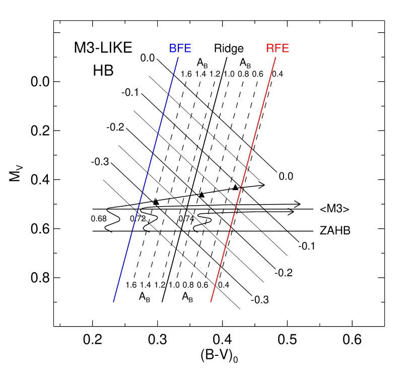
Figure 1: The instability strip in the HR diagram relevant for RRL variables from $0<M_{V}<+1$. The blue and red edges of the strip and the mid-ridge line for RRab fundamental pulsators are from Equations (1)–(3). The intercepts in these equations are set by requiring $(B\!-\!V)_{0}=0.27$ and 0.42 at the strip edges for $M_{V}({\rm mean\ evolved})=0.52$, based on CCD data for M3 (CCC05). The lines of constant period are put with a slope of $dM_{V}/d(B\!-\!V)=2.5$. A schematic age zero HB for an M3-like HB morphology is put at $M_{V}({\rm ZAHB})=0.61$. Masses are marked next to the tracks, based on Dorman’s (1992) models. Three, more highly evolved, stars are shown schematically on these tracks as dark triangles that are repeated in later diagrams.

Figure 2: A collage of correlations for stars on the HB and evolutionary tracks in Figure 1. Panel (a) is the predicted and observed period-amplitude Bailey diagram. The solid line is the prediction by reading Figure 1 as described in the text. The Roman crosses show the ridge-line M3 observations from CCC05, listed in Table 1. Panel (b) is the same as (a) but with the observed envelope lines with $\Delta\log P=\pm 0.02\;$dex put around the central ridge-line prediction. Panel (c) is the predicted and observed M3 period-color relation implicit in Figure 1. The crosses are the observations from CCC05, listed in Table 2. Panel (d) shows the color-amplitude prediction from Figure 1 compared with the CCC05 data listed in Table 3. The envelope lines in panels (b), (c), and (d) are from the observations put at about the $\pm 1.5\sigma$ level.

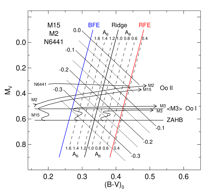
Figure 3: Grid lines of constant period and amplitude from Figure 1. The nearly horizontal HB of M3-like tracks starting from an ZAHB inside the strip are contrasted with the sloping tracks of the Oosterhoff II period group with M2 and M15 as templates, with both tracks starting from an ZAHB that is outside the strip. The slight variation of the position of the ZAHB for different metallicities over the range of [Fe/H] between $-1.5$ and $-2.2$ (VandenBerg et al., 2000; Sandage & Tammann, 2006, Figure 9) is neglected.

Figure 4: Panel (a); the observed linearized period-amplitude Bailey diagrams for the four globular clusters M3 (Oosterhoff period group I), M2 and M15 (Oosterhoff period group II), and the anomalous second parameter cluster NGC 6441. The predicted $P$-$A_{B}$ relation for M3, taken from Figure 2 is shown with the linearized M3 relation based on the observations of CCC05; (b) Predicted $A_{B}$-$P$ relations using Figure 3 for the same four clusters; (c) the observed $P$-$(B\!-\!V)_{0}$ correlation for six globular clusters showing the difference in the slopes between Oosterhoff I and II clusters; the adopted reddenings are listed; (d) predicted $P$-color correlation for M3, M2, and M15 based on Figure 3.

Figure 5: Demonstration that the slope of the color-amplitude relation, corrected for reddening, is also the same for Oosterhoff period I and II clusters. The slope, $dA_{B}/d(B\!-\!V)$, for M3 at $-8.70$ is also the same as for classical Cepheids from Equation (8).

References

- Adams & Joy (1927) Adams, W. A., & Joy, A. E. 1927, Proc. Nat. Acad. Sci., 13, 391
- Arp (1955) Arp, H. C. 1955, AJ, 60, 317
- Bingham et al. (1984) Bingham, E. A., Cacciari, C., Dickens, R. J., & Fusi Pecci, F. 1984, MNRAS, 209, 765
- Bono et al. (1997a) Bono, G., Caputo, F., Cassisi, S., Castellani, V., & Marconi, M. 1997a, ApJ, 479, 279
- Bono et al. (1997b) Bono, G., Caputo, F., Cassisi, S., Incerpi, R., & Marconi, M. 1997b, ApJ, 483, 811
- Bono et al. (2007) Bono, G., Caputo, F., & Di Criscienzo, M. 2007, A&A, 476, 779
- Brocato et al. (1996) Brocato, E., Castellani, V., & Ripepi, V. 1996, AJ, 111, 809
- Cacciari et al. (2005) Cacciari, C., Corwin, T. M., & Carney, B. W. 2005, AJ, 129, 267 (CCC05) (M3)
- Caputo et al. (1999) Caputo, F., Castellani, V., Marconi, M., & Ripepi, V. 1999, MNRAS, 306, 815
- Caputo et al. (2000) Caputo, F., Castellani, V., Marconi, M., & Ripepi, V. 2000, MNRAS, 316, 819
- Carretta et al. (2000) Carretta, E., Gratton, R. G., Clementini, G., & Fusi Pecci, F. 2000, ApJ, 533, 215
- Clement et al. (2001) Clement, C. M., et al. 2001, AJ, 122, 2587
- Cox (1974) Cox, J. P. 1974, Rep. Prog. Phys., 37, 563
- Cox (1980) Cox, J. P. 1980, Theory of Stellar Pulsation (Princeton: Princeton Univ. Press)
- Demarque et al. (2000) Demarque, P., Zinn, R., Lee, Y. W., & Yi, S. 2000, AJ, 119, 1398
- Dickens & Flinn (1972) Dickens, R. J., & Flinn, R. 1972, MNRAS, 158, 99
- Dorman (1992) Dorman, B. 1992, ApJS, 81, 221
- Fernley (1993) Fernley, J. 1993, A&A, 268, 591
- Fernley et al. (1998a) Fernley, J., Barnes, T. G., Skillen, I., Hawley, S. L., Hanley, C. J., Evans, D. W., Solano, E., & Garrido, R. 1998a, A&A, 330, 515
- Fernley et al. (1998b) Fernley, J., Carney, B. W., Skillen, I., Cacciari, C, & Janes, K. 1998b, MNRAS, 293, L61
- Gautschy & Saio (1995) Gautschy, A., & Saio, H. 1995, ARA&A, 33, 75
- Harris (1996) Harris, W. E. 1996, AJ, 112, 1487
- Iben (1967) Iben, I. 1967, ARA&A, 5, 571
- Kinman (1959) Kinman, T. J. 1959, MNRAS, 119, 538
- Lee & Carney (1999) Lee, J.-W., & Carney, B. W. 1999, AJ, 117, 2868
- Lee (1990) Lee, Y.-W. 1990, ApJ, 363, 159
- Lee et al. (1990) Lee, Y.-W., Demarque, P., & Zinn, R. 1990, ApJ, 350, 155
- McNamara (1997) McNamara, D. H. 1997, PASP, 109, 1221
- McNamara (2000) McNamara, D. H. 2000, in ASP Conf. Ser. 210, Delta Scuti and Related Stars, ed. M. Breger, M. H. Montgomery (San Francisco, CA: ASP), 373
- Olech et al. (2001) Olech, A., Kaluzny, J., Thompson, I. B., Pych, W., Krzemiński, W., & Schwarzenberg-Czerny, A. 2001, MNRAS, 321, 421
- Oosterhoff (1939) Oosterhoff, P. T. 1939, Observatory, 62, 104
- Oosterhoff (1944) Oosterhoff, P. T. 1944, Bull. Astron. Inst. Netherlands, 10, 55
- Payne-Gaposchkin (1959) Payne-Gaposchkin, C. 1959, J. Wash. Acad. Sci., 49, 333
- Payne-Gaposchkin (1961) Payne-Gaposchkin, C. 1961, in Vistas Astron. 4, ed. A. Beer (Oxford: Pergamon Press), 184
- Payne-Gaposchkin & Gaposchkin (1966) Payne-Gaposchkin, C., & Gaposchkin, S. 1966, in Vistas Astron. 8, ed. A. Beer & K. A. Strand (Oxford: Pergamon Press), 191
- Pritzl et al. (2000) Pritzl, B., Smith, H. A., Catelan, M., & Sweigart, A. V. 2000, ApJ, 530, L41
- Pritzl et al. (2001) Pritzl, B., Smith, H. A., Catelan, M., & Sweigart, A. V. 2001, AJ, 122, 2600
- Rich et al. (1997) Rich, R. M., et al. 1997, ApJ, 484, L25
- Ritter (1879) Ritter, A. 1879, Ann. Phys. Chem. Neue Folge, 8, 157
- Russell (1927) Russell, H. N. 1927, ApJ, 66, 122
- Sandage (1958) Sandage, A. 1958, in RicA, 5, Stellar Populations: The Vatican conference, ed. D. J. K. O’Connell (Amsterdam: North-Holland), 41
- Sandage (1981) Sandage, A. 1981, ApJ, 248, 161
- Sandage (1990) Sandage, A. 1990, ApJ, 350, 603 (S90)
- Sandage (1993) Sandage, A. 1993, AJ, 106, 703
- Sandage (2006) Sandage, A. 2006, AJ, 131, 1750
- Sandage et al. (1994) Sandage, A., Diethelm, R., & Tammann, G. A. 1994, A&A, 283, 111 (SDT94)
- Sandage et al. (1981) Sandage, A., Katem, B., & Sandage, M. 1981, ApJS, 46, 41
- Sandage & Tammann (2006) Sandage, A., & Tammann, G. A. 2006, ARA&A, 44, 93
- Sandage et al. (2004) Sandage, A., Tammann, G. A., & Reindl, B. 2004, A&A, 424, 43 (STR04) (LMC Cepheids)
- Sandage et al. (2009) Sandage, A., Tammann, G. A., & Reindl, B. 2009, A&A, 493, 471 (STR09) (SMC Cepheids)
- Schwarzschild (1940) Schwarzschild, M. 1940, Cir. Harv. Coll. Obs., 437, 1
- Shapley (1927a) Shapley, H. 1927, Cir. Harv. Coll. Obs., 314, 1
- Shapley (1927b) Shapley, H., & Walton, M. L. 1927, Cir. Harv. Coll. Obs., 313, 1
- Storm et al. (1991) Storm, J., Carney, B. W., & Beck, J. A. 1991, PASP, 103, 1264
- Sweigart & Catelan (1998) Sweigart, A. V., & Catelan, M. 1998, ApJ, 501, L63
- Tammann et al. (2003) Tammann, G. A., Sandage, A., & Reindl, B. 2003, A&A, 404, 423 (TSR03) (Galactic Cepheids)
- VandenBerg et al. (2000) VandenBerg, D. A., Swenson, F. J., Rogers, F. J., Iglesias, C. A., & Alexander, D. R. 2000, ApJ, 532, 430