Event-based Corpuscular Model for Quantum Optics Experiments

Abstract

A corpuscular simulation model of optical phenomena that does not require the knowledge of the solution of a wave equation of the whole system and reproduces the results of Maxwell’s theory by generating detection events one-by-one is presented. The event-based corpuscular model is shown to give a unified description of multiple-beam fringes of a plane parallel plate, single-photon Mach-Zehnder interferometer, Wheeler’s delayed choice, photon tunneling, quantum erasers, two-beam interference, double-slit, and Einstein-Podolsky-Rosen-Bohm and Hanbury Brown-Twiss experiments.

I Introduction

The theory of optical phenomena has a long and interesting history Born and Wolf (1964); Paul (2004); Garrison and Chiao (2009). The corpuscular theory of Newton and his followers was abandoned in favor of extensions pf Huygens’ wave theory, culminating in Maxwell’s theory of electrodynamics. Maxwell’s theory is extremely powerfull. It applies to virtually all electrodynamic phenomena that find practical, real-life applications. Yet, as with any theory, Maxwell’s theory has its limitations. With Einstein’s explanation of the photoelectric effect in terms of photons, that is in terms of indivisible quanta of light, the idea of a corpuscular description of light revived. Einstein’s hypothesis of light quanta gave birth to the quantum description of light. As the photoelectric effect can be explained by treating the electromagnetic field without assuming the existence of photons Garrison and Chiao (2009), the photoelectric effect itself does not indicate that light consists of indivisible particles but the experiments to be described next do.

I.1 Photon indivisability experiments

The paper by Grangier et al. Grangier et al. (1986) reports clear and direct evidence for the indivisiblity of the single photons Garrison and Chiao (2009). A key feature in this work is the use of the three-level cascade photon emission of the calcium atom. When the calcium atoms are excited to the third lowest level, they relax to the second lowest state, emitting photons of frequency $f$, followed by another transition to the ground state level causing photons of frequency $f^{\prime}$ to be emitted Kocher and Commins (1967). It is observed that each such two-step process emits two photons in two spatially well-separated directions, allowing for the cascade emission to be detected using a time-coincidence technique Kocher and Commins (1967).

In Fig. 1 we show a diagram of the first experiment reported in Ref.Grangier et al., 1986. One of two light beams produced by the cascade is directed to detector $D$. The other beam is sent through a 50-50 beam splitter to detectors $D_{0}$ and $D_{1}$. Time-coincindence logic is used to establish the emission of the photons by the three level cascade process: Only if detector $D$ and $D_{0}$, $D_{1}$ or both fire, a cascade emission event occured. Then, the absence of a coincidence between the firing of detectors $D_{0}$ and $D_{1}$ provides unambigous evidence that the photon created in the cascade and passing through the beam splitter behaves as one indivisble entity. The analysis of the experimental data strongly support the hypothesis that the photons created by the cascade process in the calcium atom are to be regarded as indivisible Garrison and Chiao (2009).

Having established the corpuscular nature of single photons, Grangier et al. Grangier et al. (1986) extend the experiment shown in Fig. 1 by sending the photons emerging from the beam splitter to another beam splitter, as illustrated in Fig. 2, thereby constructing a Mach-Zehnder interferometer (MZI). As the mirrors $M$ do not alter the particle character of the photons, the removal of the second beam splitter yields an experimental configuration that is equivalent to the one used to demonstrate the corpuscular nature of single photons. With the second beam splitter in place, Grangier et al. Grangier et al. (1986) observe that after collecting many photons one-by-one, the detection counts fit nicely to the interference curve that is predicted by Maxwell’s theory, that is what they observe is the same result as if the source would have emitted a wave. Thus, it is shown that one-by-one these particles can build up an interference pattern, just as in the experiment with single-electrons Merli et al. (1976); Tonomura et al. (1989); Tonomura (1998), for instance.

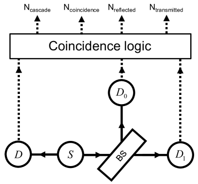
Figure 1: Schematic diagram of the first experiment reported in the paper by Grangier et al. Grangier et al. (1986), demonstrating the indivisiblity of the photon. S: Light source; BS: 50-50 beam splitter; $D$, $D_{0}$, $D_{1}$: Detectors $N_{\mathbf{cascade}}$: Number of excitations of the three-level cascade of the calcium atoms in the source S; $N_{\mathbf{coincidence}}$: Number of times detector $D_{0}$ and $D_{1}$ fire within a time window relative to the excitation of the cascade Grangier et al. (1986); $N_{\mathbf{reflectied}}$: Number of photons reflected by the BS; $N_{\mathbf{transmitted}}$: Number of photons transmitted by the BS. Solid lines: Flow of photons. Dashed lines: Flow of data.

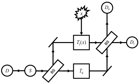
Figure 2: Schematic diagram of the second experiment reported in the paper by Grangier et al. Grangier et al. (1986), demonstrating that photons build up an interference pattern one by one. S: Light source; BS: 50-50 beam splitter; $T_{0}$: Fixed time-of-flight; $T_{1}(x)$: Variable time-of-flight controlled by the external variable $x$; $D_{0}$, $D_{1}$: Detectors. For clarity, the coincidence logic (see Fig. 2) has been omitted.

I.2 Particles, waves or magic?

In summary, the experimental observations lead to the conclusions that

1. Individual photons are indivisible

2. In a MZI, the collection of many individual photons produces the interference pattern that is expected from classical wave theory.

The conjuction of these two conclusions cannot be explained within Maxwell’s theory or quantum theory. This is most obvious in the case of Maxwell’s theory which does not pretend to describe particles. Imagining a single photon to be a spatially localized excitation of a wave field, this so-called wave packet would, according to wave theory, be divided into two wave packet by a beam splitter. This is not what is observed in the experiments of Grangier et al. Grangier et al. (1986).

Particle-wave duality, a concept of quantum theory which attributes to photons the properties of both wave and particle depending upon the circumstances, does not help to explain the experimental facts either. The experiments Grangier et al. (1986) show that each individual photon behaves as a particle, not as a wave. In these experiments (and in many others that use single-photon sources), it is clear that one particular photon never interferes with itself nor with other ones; the wave functions that are used in the wave mechanical theory interfere if they interact with material only Roychoudhuri (2010). It is only in the mathematical, statistical description of many detected photons that (probability) waves interfere Mandel (1999).

As a last resort to explain the experimental facts using concepts of quantum theory the idea of wavefunction collapse von Neumann (1955) is often used. According to this idea, the wavefunction materializes into a particle during the act of measurement. The mechanism that gives rise to this collapse has remained elusive for 78 years after of its conception. Therefore, with the present state of understanding, invoking the wavefunction collapse to explain an experimental observation adds a flavor of mysticism to the explanation. It is important to note that the mystical element never enters a quantum theory calculation of the statistical averages Ballentine (2003) and is, for any practical purpose, superfluous. It only serves to create the illusion that quantum theory has something meaningfull to say about an individual event but this is not the case. Quantum theory gives us a recipe to compute the frequencies (averages) for observing events but does not describe individual event themselves Home (1997). Of course, the introduction of a mystical element is undesirable from a scientific viewpoint and, as shown in the present paper, also unnecessary to explain the observed phenomena.

I.3 Aim of this work

The present work is based on three assumptions, namely

1. A photon is an indivisible entity.

2. Photons do not interact.

3. The result of many photons recorded by a detector is described by Maxwell’s theory.

Obviously, there is strong emperical evidence for all these three assumptions. As explained earlier, the conjunction of assumption 1 and 3 poses some serious conceptual problems that cannot be resolved within quantum theory proper.

In this paper, we show that quantum optics experiments which are performed in the single-photon regime (as in the experiments discussed in Section I.1), can be explained entirely

• with a universal event-based corpuscular model,

• without first solving a wave equation,

The event-based corpuscular model (EBCM) that we introduce in this paper is universal in that it can, without modification, be used to explain why photons build up interference patterns, why they can exhibit correlations that cannot be explained within Maxwell’s theory and so on.

The EBCM gives a cause-and-effect description for every step of the process, starting with the emission and ending with the detection of the photon. By construction, the EBCM satisfies Einstein’s criterion of local causality. Although not essential, an appealing feauture of the EBCM is that it allows for a realistic interpretation of the variables that appear in the simulation model. The research presented in this paper unifies and extends earlier work De Raedt et al. (2005a, b, c); Michielsen et al. (2005); De Raedt et al. (2006a, 2007a, 2007b, 2007c); Zhao and De Raedt (2008); Zhao et al. (2008a, b); Jin et al. (2010a, b, c).

I.4 Disclaimer

The present paper is not concerned with an interpretation or an extension of quantum theory. The existence of an EBCM for event-based phenomena does not affect the validity and applicability of quantum theory or Maxwell’s theory but shows that it is possible to give explanations of observed phenomena that do not find a logically consistent, rational explanation within these two theories.

I.5 Structure of the paper

The paper is organized as follows. In Section II, we examine the question of particle-versus-wave from a computational point of view. We show that also from this viewpoint, there are conceptual difficulties to merge the wave description in terms of probability amplitudes with the fact that detectors “click”. Section III discusses the general ideas that underpin our event-by-event simulation approach. In Section IV we introduce the EBCM of the interface between two media and of the detector, that is we define the algorithms that will be used in the particle-by-particle simulation. Section V is devoted to the validation of the EBCM: It is shown that it reproduces the results of Maxwell’s theory for a simple interface, a plane-parallel plate, and the double-slit experiment, without changing the algorithms of course. Building on the EBCM of the interface, Section IV specifies the EBCM of the optical components that are used in (quantum) optics. In Section VII, we show that the same EBCM reproduces, event-by-event and without using the solution of a wave equation, Mach-Zehnder interferometer experiments Grangier et al. (1986), Wheeler’s delayed choice experiment Jacques et al. (2007), quantum eraser Schwindt et al. (1999) and photon tunneling experiments Mizobuchi and Ohtaké (1992); Unnikrishnan and Murthy (1996); Brida et al. (2004). Section VIII shows that the EBCM approach effortlessly extends to experiments with correlated photons by showing that it reproduces the quantum theory results of the Einstein-Podolsky-Rosen-Bohm (EPRB) experiments with photons Aspect et al. (1982a, b); Weihs et al. (1998) and Hanbury Brown-Twiss (HBT) experiments. Our conclusions and a discussion of open problems are given in Section IX.

II Computational point of view

Our approach employs algorithms, that is we define processes, that contain a detailed specification of each individual event which, as we now show by an explicit example, cannot be derived from a wave theory such as Maxwell’s theory or quantum theory.

To understand the subtleties that are involved, it is helpful to consider as a simple example, the conventional wave theoretical description of the Mach-Zehnder interferometer.

II.0.1 Mach-Zehnder interferometer

A schematic diagram of a MZI experiment is shown in Fig. 2. We assume that the length $L_{0}=cT_{0}$ of the lower arm of the interferometer is fixed and that the length $L_{1}(x)=cT_{1}(x)$ of the upper arm can be varied by changing the control variable $x$.

Assuming a coherent monochromatic light source $S$ with frequency $\omega$ and a fixed value $x$, it follows from Maxwell’s theory Born and Wolf (1964) that the electric-field amplitudes $b_{0}$ and $b_{1}$ on detectors 0 and 1 are related to the input amplitudes $a_{0}$ and $a_{1}$ by

$$\left(\begin{array}[]{c}b_{0}\\ b_{1}\end{array}\right) = \frac{1}{2}\left(\begin{array}[]{cc}1&i\\ i&1\end{array}\right)\left(\begin{array}[]{cc}e^{i\phi_{0}}&0\\ 0&e^{i\phi_{1}}\end{array}\right)\left(\begin{array}[]{cc}1&i\\ i&1\end{array}\right)\left(\begin{array}[]{c}a_{0}\\ a_{1}\end{array}\right),$$ (11)

$$\equiv ABA\left(\begin{array}[]{c}a_{0}\\ a_{1}\end{array}\right),$$ (14)

where

$$A=\frac{1}{\sqrt{2}}\left(\begin{array}[]{cc}1&i\\ i&1\end{array}\right)\quad,\quad B=\left(\begin{array}[]{cc}e^{i\phi_{0}}&0\\ 0&e^{i\phi_{1}}\end{array}\right),$$ (19)

where $\phi_{0}=\omega T_{0}$ and $\phi_{1}(x)=\omega T_{1}(x)$. As the light enters the MZI via port 0 of the left most BS, we have $a_{0}=1$ and $a_{1}=0$ up to an irrelevant phase factor. Then, according to quantum theory, the probabilities $P_{0}$ ($P_{1}$) for detectors $D_{0}$ or (exclusive) $D_{1}$ to generate a click, are given by

$$P_{k}=\left|\sum_{j=0,1}\sum_{i=0,1}A_{k,j}B_{j,i}A_{i,0}\right|^{2}\quad,\quad k=0,1,$$ (20)

respectively.

Using Eqs. (14) and (20) a simple calculation yields a closed form expression for $P_{k}$, namely

$$P_{0} = \sin^{2}\frac{\omega(T_{0}-T_{1}(x))}{2}=\sin^{2}\frac{\phi_{0}-\phi_{1}(x)}{2},$$ (21)

$$P_{1} = \cos^{2}\frac{\omega(T_{0}-T_{1}(x))}{2}=\cos^{2}\frac{\phi_{0}-\phi_{1}(x)}{2}.$$ (22)

Equations (21) and (22) show that the signal on the detectors is modulated by the difference between the time-of-flights $T_{0}$ and $T_{1}(x)$ in the lower and upper arm of the interferometer, respectively, or in other words by the phase difference $\phi_{0}-\phi_{1}(x)$. This modulation is characteristic for interference phenomena.

II.0.2 Using the solution of wave theory

Once we know $P_{k}$, it is trivial to construct a process that generates clicks of the detectors $D_{0}$ and $D_{1}$. For instance, if we want to mimic the unpredictable character of the single-photon detection process, we may use a pseudo-random number generator to produce detection events. It is irrelevant whether we have a closed form expression for $P_{k}$ or only know $P_{k}$ in tabulated form. The key point is that we worked out the sums over the indices $i$ and $j$ in Eq. (20) ourselves, and that the solution of the full wave mechanical problem is used to produce the events.

II.0.3 Fundamental problem: Example

Let us now assume that we do not know how to perform the sums over the indices $i$ and $j$ in Eq. (20). In other words, we assume that we do not know the explicit (or tabulated) form of $P_{0}$ and $P_{1}$. Then, we cannot simply use the pseudo-random number generator to generate detector clicks.

Of course, we can still construct discrete-event processes that perform the sums in Eq. (20) by selecting (one-by-one) the pairs $(i,j)$ from the set ${\cal S}={(0,0),(1,0),(0,1),(1,1)}$. Any such process defines a sequence of “events” $(i,j)$. The key question now is: Can we identify the selection of the pairs with “clicks” that correspond to detection events? We now provide a trivial, rigorous proof that this is fundamentally impossible.

A characteristic feature of all wave phenomena is that not all contributions to the sums in Eq. (20) have the same sign: In wave theory, this feature is essential to account for destructive interference. But, at the same time this feature forbids the existence of a process of which the “events” can be identified with the clicks of the detector.

This is easily seen by considering a situation in which, for instance, $P_{0}=0$. In this case, the detector $D_{0}$ should never click. However, according to Eq. (20), any process that samples from the set ${\cal S}$ produces “events” such that the sum over all these “events” vanishes. Therefore, if we want to identify these “events” with the clicks that we observe, we run into a logical contradiction: To perform the sums in Eq. (20), we have to generate events that in the end cannot be interpreted as clicks since in this particular case no detector clicks are observed.

II.0.4 Fundamental problem: Generic case

From the point of view of wave theory, the example of the MZI, though very simple, is generic: Charateristic of Maxwell’s theory and quantum theory  is that the observable phenomena are described by expressions, such as Eq. (20), that involve taking the square of the sum over amplitudes that are real or complex valued. In general, these expressions take the form

$$P_{i_{n+1},i_{0}}=\left|\sum_{\{i_{1},\ldots,i_{n}\}}A_{i_{n+1},i_{n}}^{(n)}\ldots A_{i_{1},i_{0}}^{(1)}\right|^{2},$$ (23)

where the elements of the matrices $A^{(j)}$ are, in general, complex valued, and the sums over the indices $i_{j}$ can take discrete values or, as in the case of a path integral, can be continuous variables.

As one or more of the $P_{i_{n+1},i_{0}}$’s may be zero, the logically inescapable conclusion is that the individual terms that appear in Eq. (23) do not contain the necessary ingredients to define a process that generates elements of the set $\{i_{1},\ldots,i_{n}\}$ if each such element is to correspond to an observable (in experiment) event.

It is of interest to note that if the matrices $A^{(j)}$ would have all non-negative entries, each element of the set $\{i_{1},\ldots,i_{n}\}$ would make a non-negative contribution to the total and hence, it is possible to associate an event to each $n$-tuple $(i_{1},\ldots,i_{n})$. Of course, in this case, the events can never form the interference patterns that are characteristic of wave phenomena.

II.0.5 A way out

The crux of our event-by-event simulation approach is that we do not start from an expression such as Eq. (23) but construct a classical, dynamical, event-by-event process that, while generating events that correspond to the observed events, produces these events with a frequency distributions that converges to the unknown (by assumption) probability distribution $P_{i_{n+1},i_{0}}$.

Initially, the system does not know about this limiting distribution and hence, during a transient period, the frequencies with which events are generated do not necessarily agree with this limiting distribution. However, as ample numerical simulations demonstrate, for many events, these first few “wrong” events do not significantly contribute to the averages and are therefore irrelevant for the comparison of the event-based simulation results with those of a wave theory.

III Event-by-event simulation

Our event-based simulation approach is unconventional in that it does not require knowledge of the wave amplitudes obtained by first solving a wave mechanical problem. Instead, the detector clicks are generated event-by-event by locally causal, adaptive, classical dynamical systems. In this section, we discuss the general aspects of our simulation approach.

The event-by-event simulation algorithms are most easily formulated in terms of messengers that carry messages and units that accept messengers, process their messages and send the messengers with a possibly modified message to the next unit. A source is a simple unit that creates messengers with specified messages on demand. A message consists of a set of numbers, conveniently represented by a vector. A messenger that appears at the output of a detection unit corresponds to an event observed in experiment. The processing units mimic the role of the optical components in the experiment and the network by connecting the processing units represents the complete experimental setup.

Within the realm of quantum optics experiments, in a pictorial description, the photon is regarded as a messenger, carrying a message that represents its time-of-flight (phase) and polarization. In this pictorial description, we may speak of “photons” generating the detection events. However, these so-called photons, as we will call them in the following, are elements of a model or theory for the real laboratory experiment only. The only experimental facts are the settings of the various apparatuses and the detection events. What happens in between activating the source and the registration of the detection events belongs to the domain of imagination.

In general, a processing unit consist of an input stage, a transformation stage and an output stage. The input (output) stage may have several ports at (through) which messengers arrive (leave). As a messenger arrives at an input port of a processing unit, the input stage updates its internal state, also represented by a vector. This update mechanism renders the unit adaptive and is essential for the simulation approach to reproduce the results of wave mechanics. For reasons that are explained later, this input stage is called deterministic learning machine (DLM). Next, the message together with the internal state of the unit are passed to the transformation stage that implements the operation of the particular device. Finally, a new message is sent to the output stage which selects the output port through which the messenger will leave the unit. Some processing units are simpler in the sense that the input stage may be omitted, in which case the unit lacks adaptivity. The rule to decide which type of unit to employ is simple: If the unit should be able to deal with “interference phenomena” , it should be adaptive, otherwise we may (but do not have to) use the simpler device. Interfaces between materials of different index of refraction, beams splitters and the like belong to the first class. A device that causes a time delay only belongs to the second class.

A very important feature of our simulation approach is that at any given time, there is only one messenger being routed through the whole network. Therefore there can be no direct communication between the messengers. As the internal state of a unit may depend on the messages it has already processed, a unit can modify the messenger and its message. It is this mechanism that can cause “interference without waves”. From this general description of the simulation algorithm, it should already be clear that the process that is being generated by the network of processing units is locally causal in Einstein’s sense.

The processing units that are essential for our approach to reproduce the results of a wave theory are simple, locally causal, classical dymamical systems defined by an update rule that specifies how the unit updates its internal state based on an incoming message. Such a unit exhibits an elementary form of learning capability and operates deterministically and is therefore called a DLM De Raedt et al. (2005b).

As dynamical systems, DLMs are interesting in their own right, in particular because they may be used for applications that have no relation to physics De Raedt et al. (2005b). In appendix A, we introduce them in a context-free manner.

IV Simulation model

In this section, we give a detailed description of the EBCM of basic optical components, the interface between to media and single-photon detectors. For simplicity of presentation, we consider materials for which the permittivity is real and the permeability is one, that is we consider ideal dielectrics only.

IV.1 Messenger and message

As we want to construct an EBCM that reproduces the results of Maxwell’s theory and the plane wave is a central concept in Maxwell’s theory Born and Wolf (1964), it makes sense to define the messenger and the message such that there is a one-to-one mapping onto the properties of the plane wave. Therefore, we briefly review the properties of plane electromagnetic waves propagating in a homogeneous medium and then show how to construct an EBCM that reproduces these properties without using wave mechanics.

The EBCM that we introduce in this paper is not a complete event-based model for all electrodynamic phenomena. The focus of this paper is on optics experiments in which the indivisabile nature of the photons is of central importance. In accordance with the classical theory of optics Born and Wolf (1964), for simplicity, we therefore ignore the interaction of electromagnetic radiation with the magnetic degrees of freedom of the materials. It is however not difficult to incoporate these interactions in the EBCM: All that is needed is to add more data to the message carried by the messengers and to define the appropriate transformation rules.

IV.1.1 Plane waves in Maxwell’s theory

A plane wave is fully specified by its wave vector $\mathbf{q}$ and the amplitudes and phases of the electric field components that are in the plane orthogonal to $\mathbf{q}$. These amplitudes and phases determine the intensity and polarization of the electromagnetic wave. The amplitudes oscillate in time with a common frequency $f$ which is related to the magnitude of the wave vector $q=|\mathbf{q}|$ and the phase velocity $v$ by $q=2\pi f/v$, see Ref. Born and Wolf (1964). In vacuum $v$ equals the speed of light $c$. If the plane wave propagates through a dielectric material, its velocity is given by $v=c/n$ where $n$ is a real number, the index of refraction of the material. Note that $v$ and $n$ are determined indirectly via the law of refraction Born and Wolf (1964).

For a plane wave traveling along the $z$-direction, the amplitudes of the non-zero electric field components can be written as Born and Wolf (1964)

$$E_{1}(\mathbf{r},t) = a_{1}\cos(\tau+\delta_{1})$$

$$E_{2}(\mathbf{r},t) = a_{2}\cos(\tau+\delta_{2}),$$ (24)

where the $1$-$2$ coordinate system can be chosen freely as long as it lies in the plane orthogonal to $z$ and $\tau=2\pi ft-\mathbf{q}\cdot\mathbf{r}$ where $\mathbf{r}$ denotes the position in 3D space. The prefactors $a_{1}$ and $a_{2}$ determine the intensity of the plane wave and together with the phase difference $\delta=\delta_{1}-\delta_{2}$ also determine its polarization Born and Wolf (1964).

In Maxwell’s theory, the amplitudes $a_{1}$ and $a_{2}$ determine the light intensity whereas in an EBCM, each messenger is assumed to contributes one unit of light to the total light intensity. Let us therefore rescale the fields $E_{1}$ and $E_{2}$ such that the average power of the $E$-field is one half. We have

$$\frac{E_{1}(\mathbf{r},t)}{\sqrt{a_{1}^{2}+a_{2}^{2}}} = \sin\xi\cos(\tau+\delta_{1})$$

$$\frac{E_{2}(\mathbf{r},t)}{\sqrt{a_{1}^{2}+a_{2}^{2}}} = \cos\xi\cos(\tau+\delta_{2}),$$ (25)

where $\sin\xi=a_{1}/\sqrt{a_{1}^{2}+a_{2}^{2}}$ and $\cos\xi=a_{2}/\sqrt{a_{1}^{2}+a_{2}^{2}}$. Expressing the Stokes parameters Born and Wolf (1964) $s_{0}=a_{1}^{2}+a_{2}^{2}$, $s_{1}=a_{1}^{2}-a_{2}^{2}$, $s_{2}=2a_{1}^{2}a_{2}^{2}\cos\delta$, $s_{3}=2a_{1}^{2}a_{2}^{2}\sin\delta$ in terms of the angles $\xi$ and $\delta$ yields $s_{1}/s_{0}=-\cos 2\xi$, $s_{2}/s_{0}=\sin 2\xi\cos\delta$, $s_{3}/s_{0}=\sin 2\xi\sin\delta$, demonstrating that Eq. (25) is just another representation of a plane monochromatic electromagnetic wave.

IV.1.2 Definition of messenger and message

The particle is regarded as a messenger, traveling with velocity $v$ in the direction $\mathbf{q}/q$. Each messenger carries with it two harmonic oscillators that vibrate with frequency $f$.

It may be tempting, but it is definitely wrong, to regard the messenger+message as a plane wave with wave vector $\mathbf{q}$, the oscillators being the two electric field components in the plane orthogonal to $\mathbf{q}$. As there is no communication/interaction between the messengers there can be no wave equation (i.e. no partial differential equation) that enforces a relation between the messages carried by different messengers. Indeed, the oscillators carried by a messenger never interact with the oscillators of another messenger, hence the motion of these pairs of oscillators is not governed by a wave equation. Naively, one might imagine the oscillators tracing out a wavy pattern in space as they travel though space. However, as there is no relation between the times at which the messengers leave the source, it is impossible to characterize all these traces by a field that depends on one set of space-time coordinates, as required for a wave theory.

There are many different but equivalent ways to define the message. As in Maxwell’s theory and quantum theory, it is convenient (though not essential) to work with complex-valued vectors, that is with messages represented by two-dimensional unit vectors

$$\mathbf{y}=\left(\begin{array}[]{c}e^{i\psi^{(1)}}\sin\xi\\ e^{i\psi^{(2)}}\cos\xi\end{array}\right).$$ (26)

where $\psi^{(i)}=2\pi ft+\delta_{i}$ for $i=1,2$. Note that, unlike in the case of waves, there is no $\mathbf{q}\cdot\mathbf{r}$ contribution to $\psi^{(i)}$. The angle $\xi$ determines the relative magnitude of the two components, which we call the polarization of the message $\mathbf{y}$.

A messenger with message $\mathbf{y}$ at time $t$ and position $\mathbf{r}$ that travels along the direction $\mathbf{q}$ during a time interval $t^{\prime}-t$, changes its message according to

$$\psi^{(i)}\leftarrow\psi^{(i)}+\phi\quad,\quad i=1,2,$$ (27)

where $\phi=2\pi f(t^{\prime}-t)$.

From Eq. (27), as the messenger moves, it changes its message by applying to the vectors $(\cos\psi^{(1)},\sin\psi^{(1)})$ and $(\cos\psi^{(2)},\sin\psi^{(2)})$ the same plane rotation

$$R(\phi)=\left(\begin{array}[]{cc}\cos\phi&{-}\sin\phi\\ \sin\phi&\phantom{-}\cos\phi\end{array}\right).$$ (28)

This suggests that we may view these two-component vectors as the coordinates of two local oscillators, carried along by the messengers. In this pictorial description, the messenger encodes its time-of-flight in these two oscillators.

IV.1.3 Remarks

Recall that in Maxwell’s theory, the energy of the electromagnetic field is encoded in the amplitudes of the wave components. In contrast, in the event-based corpuscular approach, the energy of the electromagnetic field is encoded in the amount of particles that crosses an unit area per unit of time.

The representation of the messages as a vector with two complex-valued components is convenient, not only to describe the propagation in a homogenous medium but, as we will see later, also to describe the effect of for instance a beam splitter, a polarizing beam splitter and so on. In essence, the interaction of the messenger with a material will change the message $y$ by applying some transformation to it. However, there is no rational argument to use the representation Eq. (26) other than that it is convenient. Any other representation, such as the ones used in our earlier papers work equally well.

When a messenger is created, its message needs to be initialized, that is we have to specify the three angles $\psi^{(1)}$, $\psi^{(2)}$, and $\xi$. This specification depends on the kind of light source we want to simulate. For instance, to simulate a coherent light source, the three angles should be the same for all messengers that are being created. Other choices are discussed when we consider specific experiments.

IV.2 Interface between two dielectric media

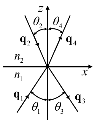
Figure 3: Refraction and reflection at a boundary between two dielectric materials with indices of refraction $n_{1}$ and $n_{2}$. The vectors $\mathbf{q}_{1}$, $\mathbf{q}_{2}$, $\mathbf{q}_{3}$, and $\mathbf{q}_{4}$ lie in the $x$–$z$ plane.

The reflection and transmission of light by a boundary that separates two homogeneous media of different optical properties is one of the basic phenomena in optics. We briefly review the wave theoretical treatment of this problem and explain how we construct the corresponding EBCM.

IV.2.1 Wave theory

In Maxwell’s theory, assuming incident plane waves from both sides of the interface (see Fig. 3), the directions and amplitudes of the reflected and transmitted plane wave follow from conservation of energy and the continuity of the tangential field components at the boundary, yielding Snell’s law and Fresnel’s formulas, respectively.

In Maxwell’s theory, Snell’s law follows from the kinematic properties of the waves. Conservation of momentum in the $x$-direction implies $q^{(1)}_{x}=q^{(2)}_{x}=q^{(3)}_{x}=q^{(4)}_{x}$. Using the relation between the frequency $f$ of the oscillations and the length of the wave vectors we find

$$\frac{2\pi f}{c}=\frac{q^{(1)}}{n_{1}}=\frac{q^{(2)}}{n_{2}}=\frac{q^{(3)}}{n_{1}}=\frac{q^{(4)}}{n_{2}},$$ (29)

where

$$q^{(i)}=\sqrt{(q^{(i)}_{x})^{2}+(q^{(i)}_{z})^{2}}\quad,\quad i=1,2,3,4,$$ (30)

from which

$$n_{1}\frac{q^{(1)}_{x}}{q^{(1)}}=n_{2}\frac{q^{(2)}_{x}}{q^{(2)}}=n_{1}\frac{q^{(3)}_{x}}{q^{(3)}}=n_{2}\frac{q^{(4)}_{x}}{q^{(4)}},$$ (31)

which is Snell’s law in its more familiar form

$$n_{1}\sin\theta_{1}=n_{2}\sin\theta_{2}=n_{1}\sin\theta_{3}=n_{2}\sin\theta_{4}.$$ (32)

For later use, we introduce the symbols $\widehat{q}^{(i)}=\mathbf{q}^{(i)}_{z}/{q}^{(i)}=(-1)^{i}\cos\theta_{i}$ for $i=1,2,3,4$, $n_{3}=n_{1}$ and $n_{4}=n_{2}$. Note that we also have $\theta_{3}=\theta_{1}$, $\theta_{4}=\theta_{2}$, $\widehat{q}^{(3)}=-\widehat{q}^{(1)}$, and $\widehat{q}^{(2)}=-\widehat{q}^{(4)}$. The kinematic properties of the particles in the EBCM are assumed to be the same as those of the waves in Maxwell’s theory.

In Maxwell’s theory the dynamics properties are contained in the boundary conditions of the electromagnetic fields at the interface. If $A_{i}$ denotes the electric-field amplitude of the plane wave with wave vector $\mathbf{q}^{(i)}$, these boundary conditions enforce the relations

$$\left(\begin{array}[]{c}A_{3}\\ A_{4}\end{array}\right)=\left(\begin{array}[]{lr}r_{12}&t_{21}\\ t_{12}&-r_{12}\end{array}\right)\left(\begin{array}[]{c}A_{1}\\ A_{2}\end{array}\right).$$ (33)

The reflection and transmission coefficients are Born and Wolf (1964)

$$r_{12} = \frac{n_{1}\widehat{q}^{(1)}-n_{2}\widehat{q}^{(4)}}{n_{1}\widehat{q}^{(1)}+n_{2}\widehat{q}^{(4)}}$$

$$t_{12} = \frac{2n_{1}\widehat{q}^{(1)}}{n_{1}\widehat{q}^{(1)}+n_{2}\widehat{q}^{(4)}}$$

$$t_{21} = \frac{2n_{2}\widehat{q}^{(4)}}{n_{1}\widehat{q}^{(1)}+n_{2}\widehat{q}^{(4)}},$$ (34)

for $S$-polarized waves and

$$r_{12} = \frac{n_{1}\widehat{q}^{(4)}-n_{2}\widehat{q}^{(1)}}{n_{1}\widehat{q}^{(4)}+n_{2}\widehat{q}^{(1)}}$$

$$t_{12} = \frac{2n_{1}\widehat{q}^{(1)}}{n_{1}\widehat{q}^{(4)}+n_{2}\widehat{q}^{(1)}}$$

$$t_{21} = \frac{2n_{2}\widehat{q}^{(4)}}{n_{1}\widehat{q}^{(4)}+n_{2}\widehat{q}^{(1)}},$$ (35)

for $P$-polarized waves.

In Maxwell’s theory the wave amplitudes are only convenient calculational tools: Observable effects are related to the energy current per unit area Born and Wolf (1964), the Poynting vectors $\mathbf{S}^{(i)}=cn_{i}\mathbf{q}^{(i)}|A_{i}|^{2}/4\pi|\mathbf{q}^{(i)}|$.

It is not difficult to rewrite Eq. (33) such that it directly relates to physical observables. Define the “energy-current amplitude” $\widetilde{A}_{i}=(cn_{i}|\widehat{q}^{(i)}|/4\pi)^{1/2}A_{i}$ and the transformation matrix $R$ by

$$R=\left(\begin{array}[]{lr}(cn_{1}\widehat{q}^{(1)}/4\pi)^{-1/2}&0\\ 0&(cn_{2}\widehat{q}^{(2)}/4\pi)^{-1/2}\end{array}\right).$$ (36)

Then, from Eq. (33) it follows that

$$\left(\begin{array}[]{c}\widetilde{A}_{3}\\ \widetilde{A}_{4}\end{array}\right) = R^{-1}\left(\begin{array}[]{lr}r_{12}&t_{21}\\ t_{12}&-r_{12}\end{array}\right)R\left(\begin{array}[]{c}\widetilde{A}_{1}\\ \widetilde{A}_{2}\end{array}\right),$$ (43)

$$= \left(\begin{array}[]{lr}\widetilde{r}&\widetilde{t}\\ \widetilde{t}&-\widetilde{r}\end{array}\right)\left(\begin{array}[]{c}\widetilde{A}_{1}\\ \widetilde{A}_{2}\end{array}\right)\equiv\widetilde{T}\left(\begin{array}[]{c}\widetilde{A}_{1}\\ \widetilde{A}_{2}\end{array}\right),$$ (50)

where $\widetilde{r}$ and $\widetilde{t}$ are given by

$$\widetilde{r}_{S} = \frac{n_{1}\widehat{q}^{(1)}-n_{2}\widehat{q}^{(4)}}{n_{1}\widehat{q}^{(1)}+n_{2}\widehat{q}^{(4)}}$$

$$\widetilde{t}_{S} = \frac{2\sqrt{n_{1}n_{2}\widehat{q}^{(1)}\widehat{q}^{(4)}}}{n_{1}\widehat{q}^{(1)}+n_{2}\widehat{q}^{(4)}},,$$ (51)

and

$$\widetilde{r}_{P} = \frac{n_{1}\widehat{q}^{(4)}-n_{2}\widehat{q}^{(1)}}{n_{1}\widehat{q}^{(4)}+n_{2}\widehat{q}^{(1)}},$$

$$\widetilde{t}_{P} = \frac{2\sqrt{n_{1}n_{2}\widehat{q}^{(1)}\widehat{q}^{(4)}}}{n_{1}\widehat{q}^{(4)}+n_{2}\widehat{q}^{(1)}},$$ (52)

in the case of $S$-polarized and $P$-polarized waves, respectively. From Eqs. (35), (51) and (52) it follows directly that $\widetilde{r}^{2}+\widetilde{t}^{2}=1$ and that the matrix $\widetilde{T}$ is unitary (with determinant minus one). As $\widetilde{T}$ is unitary we have $|\widetilde{A}_{3}|^{2}+|\widetilde{A}_{4}|^{2}=|\widetilde{A}_{1}|^{2}+|\widetilde{A}_{2}|^{2}$, that is the total energy of the incident waves is equal to the total energy of the outgoing waves, as it should be.

Clearly, in an EBCM of refraction and reflection at a dielectric, lossless interface, there can be no loss of particles: An incident particle must either bounce back from or pass through the interface. If the EBCM is to reproduce the results of Maxwell’s theory  the boundary conditions on the wave amplitudes in Maxwell’s theory must translate into a rule that determines how a particle bounces back or crosses the interface. But in the EBCM there are only particles, no wave amplitudes. However, as we have seen in Maxwell’s theory the wave energies, not the wave amplitudes, appear in conservation laws. This suggests that in an EBMC, we should use the matrix $\widetilde{T}$ to transform the message carried by the messenger.

IV.2.2 EBCM of the interface

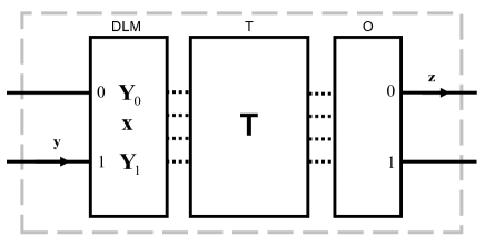
Figure 4: Diagram of a DLM-based processing unit that performs an event-based simulation of optical components. The processing unit consists of three stages: An input stage (DLM), a transformation stage (T) and an output stage (O). The solid lines represent the input and output ports of the device. The presence of a message is indicated by an arrow on the corresponding port line. The dashed lines indicate the data flow within the unit. The transformation matrix ${\bf T}$ is component specific.

We now have all ingredients to construct the processing unit that performs the event-by-event, corpuscular simulation of refraction and reflection of light at a dielectric, lossless interface.

The processing unit has the generic structure, depicted in Fig. 4, consisting of an input stage (DLM), a transformation stage (T), and an output stage (O) De Raedt et al. (2005a, b, c); Michielsen et al. (2005). There are two input and two output ports labeled by $k=0,1$. Refering to Fig. 3, input port $k=0,1$ accepts messengers travelling along directions $\mathbf{q}^{(1)}/{q}^{(1)}$ and $\mathbf{q}^{(2)}/{q}^{(2)}$, respectively (recall that at any time, only one messenger arrives at either port 0 or 1). Likewise, a messenger leaves in the directions $\mathbf{q}^{(3)}/{q}^{(3)}$ and $\mathbf{q}^{(4)}/{q}^{(4)}$ through output port $k=0,1$, respectively.

For simplicity, we assume that the incoming messenger is constructed such that its first oscillator vibrates in the plane that is orthogonal to the plane of incidence (the $xz$-plane in Fig. 3) while its second oscillator vibrates in the plane that is parallel to the plane of incidence, corresponding to $S$ and $P$ polarized plane waves, respectively. Note that this assumption merely amounts to a convenient choice of the coordinate system.

IV.2.3 Input stage

The DLM receives a message on either input port $0$ or $1$, never on both ports simultaneously. If we represent the arrival of a messenger at port 0 (1) by the vectors ${\bf v}=(1,0)$ or ${\bf v}=(0,1)$, it is clear that we can employ the DLM of Section .3, second case, to estimate the relative frequencies with which the messengers arrive on ports 0 or 1, respectively.

According to Section .3, a DLM that is capable of performing this task should have an internal vector $\mathbf{x}=(x_{0},x_{1})$, where $x_{0}+x_{1}=1$ and $x_{k}\geq 0$ for all $k=0,1$. In addition to the internal vector $\mathbf{x}$, the DLM needs to have two sets of two registers $\mathbf{Y}_{k}=(Y_{k,1},Y_{k,2})$ to store the last message $\mathbf{y}$ that arrived at port $k$. Thus, the DLM has storage for exactly ten real-valued numbers.

Upon receiving a messenger at input port $k$, the DLM performs the following steps: It copies the elements of message $\mathbf{y}$ in its internal register $\mathbf{Y}_{k}$

$$\mathbf{Y}_{k}\leftarrow\mathbf{y}$$ (53)

while leaving $\mathbf{Y}_{1-k}$ unchanged and replaces its internal vector according to

$$\mathbf{x}\leftarrow\gamma\mathbf{x}+(1-\gamma)\mathbf{v},$$ (54)

where $0\leq\gamma<1$. Note that each time a messenger arrives at one of the input ports, the DLM replaces the values of the internal vector $\mathbf{x}$ and of the ones in the registers $\mathbf{Y}_{k}$ by overwriting the old ones. It does not store all the messages, but only two!

IV.2.4 Transformation stage

The second stage (T) accepts a message from the input stage, and transforms it into a new message. From the description of the input stage, it is clear that the internal registers $\mathbf{Y}_{0}$ and $\mathbf{Y}_{1}$ contain the last message that arrived on input port 0 and 1 respectively. First, this data is combined with the data of the internal vector $\mathbf{x}$, the components of which converge (after many events have been processed) to the relative frequencies with which the messengers arrive on port 0 and 1, respectively. The output message generated by the input stage is

$$\left(\begin{array}[]{c}{Y}_{0,1}^{\prime}\\ {Y}_{1,1}^{\prime}\\ {Y}_{0,2}^{\prime}\\ {Y}_{1,2}^{\prime}\end{array}\right)=\left(\begin{array}[]{cccc}x_{0}^{1/2}&0&0&0\\ 0&x_{1}^{1/2}&0&0\\ 0&0&x_{0}^{1/2}&0\\ 0&0&0&x_{1}^{1/2}\end{array}\right)\left(\begin{array}[]{c}{Y}_{0,1}\\ {Y}_{1,1}\\ {Y}_{0,2}\\ {Y}_{1,2}\end{array}\right),$$ (55)

Note that as $x_{0}+x_{1}=1$ and $\|\mathbf{Y}_{0}\|=\|\mathbf{Y}_{1}\|=1$, we have $|{Y}_{0,1}^{\prime}|^{2}+|{Y}_{0,2}^{\prime}|^{2}+|{Y}_{1,1}^{\prime}|^{2}+|{Y}_{1,2}^{\prime}|^{2}=1$.

Recall that in the EBCM, the number of incoming messengers with message $\mathbf{Y}_{k}$ represents the energy-density current of the corresponding plane wave, which by construction is proportional to $|\mathbf{Y}_{k}^{\prime}|^{2}$. Therefore, according to Eq. (50), the outgoing energy-density currents are given by

$$\left(\begin{array}[]{cc}{Z}_{0,1}\\ {Z}_{1,1}\\ {Z}_{0,2}\\ {Z}_{1,2}\end{array}\right)=\mathbf{T}\left(\begin{array}[]{c}{Y}_{0,1}^{\prime}\\ {Y}_{1,1}^{\prime}\\ {Y}_{0,2}^{\prime}\\ {Y}_{1,2}^{\prime}\end{array}\right),$$ (56)

where the transformation matrix $\mathbf{T}$ is given by

$$\mathbf{T}=\left(\begin{array}[]{cccc}\widetilde{r}_{S}&\phantom{-}\widetilde{t}_{S}&0&0\\ \widetilde{t}_{S}&-\widetilde{t}_{S}&0&0\\ 0&0&\widetilde{r}_{P}&\phantom{-}\widetilde{t}_{P}\\ 0&0&\widetilde{t}_{P}&-\widetilde{r}_{P}\end{array}\right),$$ (57)

and the matrix elements are given by Eqs. (51) and (52).

IV.2.5 Output stage

The output stage (O) uses the data provided by the transformation stage (T) to decide on which of the two ports it will send out a messenger (representing a photon). The rule is very simple: We compute $z=|{Z}_{1,1}|^{2}+|{Z}_{1,2}|^{2}$ and select the output port $\widehat{k}$ by the rule

$$\widehat{k}=\Theta(z-r),$$ (58)

where $\Theta(.)$ is the unit step function and the $0\leq r<1$ is a uniform pseudo-random number (which is different for each messenger processed). The messenger leaves through port $\widehat{k}$ carrying the message

$$\mathbf{z}=\frac{1}{\sqrt{|{Z}_{\widehat{k},1}|^{2}+|{Z}_{\widehat{k},2}|^{2}}}\left(\begin{array}[]{c}{Z}_{\widehat{k},1}\\ {Z}_{\widehat{k},2}\end{array}\right),$$ (59)

which, for reasons of internal consistency, is a unit vector.

IV.2.6 Remarks

The internal vector of the DLM can be given physical meaning: It represents the polarization vector of the charge distribution of an atom. The update rule Eq. (54) defines the equation of motion of this vector. In essence, the EBCM is a simplified version of the classical Newtonion Lorentz model for the response of the polarization of an atom/molecule to the applied electric field Born and Wolf (1964), with one important difference: It describes the interaction of a single photon with the atom. The update rule Eq. (54) is not the only rule which yields an EBCM that reproduces the results of Maxwell’s theory (see Section V). The question of the correctness of the update rule can only be settled by a new type of experiment that addresses this specific question.

The use of pseudo-random numbers to select the output port is not essential De Raedt et al. (2005b): We generally use pseudo-random numbers to mimic the apparent unpredictability of the experimental data only. From a simulational point of view, there is nothing special about using pseudo-random numbers. On a digital computer, pseudo-random numbers are generated by deterministic processes anyway hence instead of a uniform pseudo-random number generator, any algorithm that selects the output port in a systematic manner might be employed as well De Raedt et al. (2005b), as long as the zero’a and one’s occur with a ratio determined by $z$. For instance, we could use the DLM described in Section .2. This will change the order in which messengers are being processed but the stationary state averages are the same.

IV.3 Single-photon detectors

Ideally, each photon that hits a single-photon detector should simply produce a signal, a click. This idealized model is used in virtually all quantum theory  modeling for very good reasons: Quantum theory postulates that the observed intensity, the average over many events, recorded by a detector is proportional to the square of the absolute value of the complex-valued wave amplitude. Likewise, Maxwell’s theory interprets the intensity of light as the energy flux (Poynting vector) per unit of time through a unit area orthogonal to the directions of the electric and magnetic field vector Born and Wolf (1964). Part of the predictive power of both wave theories stems from these postulates as they allow the calculation of intensities completely independent of the details of how the intensity is actually measured. In jargon, these theories are noncontextual Home (1997).

It is generally accepted that a description on the level of individual events necessarily entails contextuality Home (1997). Therefore, in plain words, a description that aims to go beyond quantum theory or Maxwell’s theory, that is a cause-and-effect description on the level of individual events, requires a detailed specification of the process of measurement itself Home (1997). Obviously, such a specification should capture the essence of a real detection process.

In reality, photon detection is the result of a complicated interplay of different physical processes Hadfield (2009). Therefore we briefly review some of the basic features of these processes before we discuss the detector model that we employ in our simulations.

IV.3.1 Generalities

In essence, a light detector consists of material that absorbs light. The electric charges that result from the absorption process are then amplified, chemically in the case of a photographic plate or electronically in the case of photo diodes or photomultipliers. In the case of photomultipliers or photodiodes, once a photon has been absorbed (and its energy “dissipated” in the detector material) an amplification mechanism (which requires external power/energy) generates an electric current (provided by an external current source) Garrison and Chiao (2009); Hadfield (2009). The resulting signal is compared with a threshold that is set by the experimenter and the photon is said to have been detected if the signal exceeds this threshold Garrison and Chiao (2009); Hadfield (2009). In the case of photographic plates, the chemical process that occurs when photons are absorbed and the subsequent chemical reactions that renders visible the image serve similar purposes.

In the wave-mechanical picture, the interaction between the incident electric field ${\mathbf{E}}$ and the material takes the form ${\mathbf{P}}\cdot{\mathbf{E}}$, where ${\mathbf{P}}$ is the polarization vector of the material Born and Wolf (1964). Treating this interaction in first-order perturbation theory, the detection probability reads $P_{\mathrm{detection}}(t)=\int^{t}_{0}\int^{t}_{0}\langle\langle{\mathbf{E}^{T}(t^{\prime})}\cdot{\mathbf{K}(t^{\prime}-t^{\prime\prime})}\cdot{\mathbf{E}(t^{\prime\prime})}\rangle\rangle dt^{\prime}dt^{\prime\prime}$ where ${\mathbf{K}(t^{\prime}-t^{\prime\prime})}$ is a memory kernel depending on the material only and $\langle\langle.\rangle\rangle$ denotes the average with respect to the initial state of the electric field Ballentine (2003); Garrison and Chiao (2009). Both the constitutive equation Born and Wolf (1964) ${\mathbf{P}}(\omega)=\chi(\omega){\mathbf{E}}(\omega)$ as well as the expression for $P_{\mathrm{detection}}(t)$ show that the detection process involves some kind of memory, as is most evident in the case of photographic films before development. It is important to take note that for the integration over $t^{\prime}$ and $t^{\prime\prime}$ to yield physically meaningful results, within the context of a wave theory, the interaction interval $[0,t]$ should extend over many periods of the wave Born and Wolf (1964).

An event-based model for the detector cannot be “derived” from quantum theory simply because quantum theory has nothing to say about individual events but predicts the frequencies of their observation only Home (1997). Therefore, any model for the detector that operates on the level of single events must necessarily appear as “ad hoc” from the viewpoint of quantum theory. The event-based detector models that we describe in this paper should not be regarded as realistic models for say, a photomultiplier or a photographic plate and the chemical process that renders the image. In particular, there is no need to account for the presence of a threshold (electrical or chemical) that is essential for real photon-detection systems to function properly Garrison and Chiao (2009); Hadfield (2009). In the spirit of Occam’s razor, these very simple event-based models capture the salient features of ideal (i.e. 100% efficient) single-photon detectors without making reference to the solution of a wave equation or quantum theory.

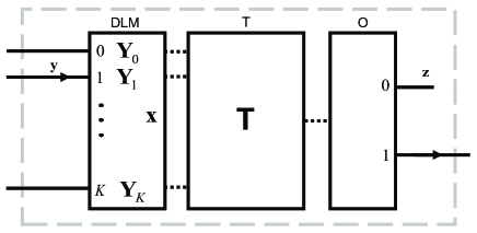
Figure 5: Diagram of the event-based detector model defined by Eqs. (60), (61), and (62). The dashed line indicates the data flow within the processing unit.

IV.3.2 EBCM of a detector

Photon detectors, such as a photographic plate of CCD arrays, consist of many identical detection units each having a predefined spatial window in which they can detect photons. In what follows, each of these identical detection units will be referred to as a detector. By construction, these detector units operate completely independently from and also do not communicate with each other.

Here we construct a processing unit that acts as a detector for individual messages. Instead of differentiating between only two different directions as in the case of the EBCM of an interface for instance, a detector should be able to process messengers that come from many different directions. The schematic diagram depicted in Fig. 5 shows that this processing unit has the same structure as the general processing unit, see Fig. 4 except that it may have more than two inputs ports. The number of input ports is denoted by $N_{p}=K+1$.

IV.3.3 Input stage

Representing the arrival of a messenger at port $0\leq k\leq K$ by the vector ${\bf v}=(v_{0},\ldots,v_{K})^{T}$ with $v_{i}=\delta_{i,k}$ the internal vector is updated according to the rule

$$\mathbf{x}\leftarrow\widehat{\gamma}\mathbf{x}+(1-\widehat{\gamma})\mathbf{v},$$ (60)

where $\mathbf{x}=(x_{0},\ldots,x_{K})^{T}$, $\sum_{k=1}^{K}x_{k}=1$, and $0\leq\widehat{\gamma}<1$. The elements of the incoming message $\mathbf{y}$ are written in internal register $\mathbf{Y}_{k}$

$$\mathbf{Y}_{k}\leftarrow\mathbf{y},$$ (61)

while all the other $\mathbf{Y}_{i}$ ($i\not=k$) registers remain unchanged. Thus, each time a messenger arrives at one of the input ports, say $k$, the DLM updates all the elements of the internal vector $\mathbf{x}$, overwrites the data in the register $\mathbf{Y}_{k}$ while the content of all other $\mathbf{Y}$ registers remains the same.

IV.3.4 Transformation stage

The output message generated by the transformation stage is

$$\mathbf{T}=\mathbf{x}\cdot\mathbf{Y}=\sum_{k=0}^{K}x_{k}\mathbf{Y}_{k},$$ (62)

which is a complex-valued two-component vector, similar to a message $\mathbf{y}$.

IV.3.5 Output stage

As in all previous event-based models for the optical components, the output stage (O) generates a binary output signal $\widehat{k}=0,1$ but unlike components such as a parallel plate, the output message does not represent a photon: It represents a “no click” or “click” if $\widehat{k}=0$ or $\widehat{k}=1$, respectively. To implement this functionality, we define (compare with Eq. (58) which is essentially the same)

$$\widehat{k}=\Theta(|\mathbf{T}|^{2}-r),$$ (63)

where $\Theta(.)$ is the unit step function and $0\leq r<1$ are uniform pseudo-random numbers (which are different for each event). The parameter $0\leq\widehat{\gamma}<1$ can be used to control the operational mode of the unit. From Eq. (63) it follows that the frequency of $\widehat{k}=1$ events depends on the length of the internal vector $\mathbf{T}$.

Note that in contrast to experiment, in a simulation, we could register both the $\widehat{k}=0$ and $\widehat{k}=1$ events. Then the sum of the $\widehat{k}=0$ and $\widehat{k}=1$ events is equal to the number of input messages. In real experiments, only $\widehat{k}=1$ events are taken as evidence that a photon has been detected. Therefore, we define the total detector count by

$$N_{\mathrm{count}}=\sum^{K}_{l=1}\widehat{k}_{l},$$ (64)

where $K$ is the number of messages received and $l$ labels the events. In words, $N_{\mathrm{count}}$ is the total number of one’s generated by the detector unit.

IV.3.6 Detection efficiency

In general, the detection efficiency is defined as the overall probability of registering a count if a photon arrives at the detector Hadfield (2009). One method to measure the detection efficiency is to use a single-photon point source, placed far away from a single detector Hadfield (2009). In an EBCM of such an experiment, all the messengers that reach the detector will approximately have the same direction, implying that these messengers arrive at this detector at the same input port, say $k$. As explained in Section .3, under these circumstances, $x_{k}$ converges exponentially to one. Hence, after receiving a few photons, the detector clicks every time a photon arrives. Thus, the detection efficiency, as defined for real detectors, of the event-based detector model is very close to 100%.

Comparing the number of ad hoc assumptions and unknown functions that enter typical quantum theory treatments of photon detectors Garrison and Chiao (2009) with the two parameters $\widehat{\gamma}$ and $N_{p}$ of the event-based detector model, the latter has the virtue of being extremely simple while providing a description of the detection process at the level of detail, the single events, which is outside the scope of quantum theory.

V Model validation

We validate the EBCM by simulating some very basic optical experiments such as reflection and refraction by a boundary between two dielectric materials and by a plane parallel plate and the interference of two light beams.

V.1 Reflection and refraction from an interface

In Fig. 6, we show the diagram and its EBCM equivalent of an experiment to measure the reflection and refraction by a boundary between two dielectric materials. In the EBCM, the source sends messengers with their initial time-of-flight set to zero to port 0 of the DLM-based processor, described in Section IV.2.2. The message consists of the vector $\mathbf{y}$ and the direction $\theta$ (or equivalently $\mathbf{q}_{1}$, see Fig. 3). The DLM-based processor accepts the message, updates its internal state according to the rules, given in Section IV.2.2. The result of this processing is that a messenger leaves the processor via port 0 or (exclusive) 1, corresponding to a reflected or transmitted messenger, respectively. The messenger then proceeds to either detector $D_{0}$ or $D_{1}$. Each detector is also a DLM-based processor (recall that we impose the condition that the same algorithms should be used in all experiments), as described in Section IV.3.2. Counting the events produced by these detectors yields the reflectivity and transmissivity of the interface.

In Fig. 7 we compare EBCM simulation results with the predictions of Maxwell’s theory Born and Wolf (1964). It is clear that there is excellent agreement, even though the number of emitted events is small compared to the number of photons used in typical optics experiments. Obviously, the EBCM passes this first test.

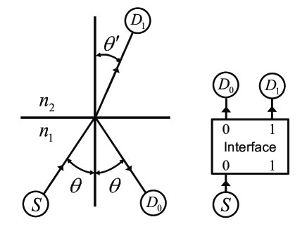
Figure 6: Diagram of the experiment to measure the reflection and refraction from an interface (left) and the diagram of the corresponding EBCM model (right). In Maxwell’s theory the source emits plane waves and the amount of energy in the reflected and transmitted light wave is recorded by detectors $D_{0}$ and $D_{1}$, respectively. In the EBCM, the source emits particles which are either reflected or refracted by the interface and the detectors $D_{0}$ and $D_{1}$ count the number of particles that are reflected or transmitted, respectively.

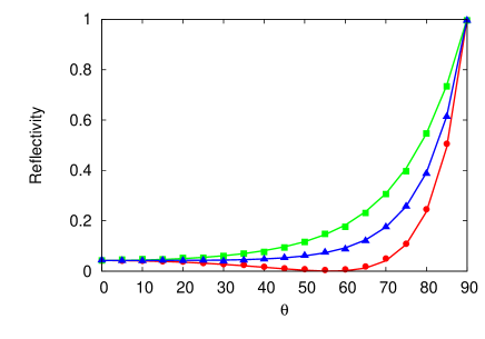
Figure 7: EBCM simulation results (markers) for the reflectivity of an interface between vacuum ($n_{1}=1$) and glass ($n_{2}=1.52$) as a function of the angle of incidence of the incoming particles (see also Fig.1.12 of Ref. Born and Wolf (1964)). The solid lines are the exact results of Maxwell’s theory Born and Wolf (1964). Green markers and lines: $\xi=0$ ($S$-polarization); Blue markers and lines: $\xi=\pi/4$ ($S$+$P$ polarization); Red markers and lines: $\xi=\pi/2$ ($P$-polarization). Simulation parameters: $10^{4}$ events per marker, $\gamma=\widehat{\gamma}=0.99$ and $N_{p}=1$.

V.2 Multiple-beam fringes with a plane-parallel plate

Light impinging on a transparant plane-parallel plate is multiply reflected at the plate boundaries, a phenomenon that has many important applications. The resulting interference effects have, according to current teaching of physics, no corpuscular analog. Therefore, this system provides a stringent testcase for the EBCM approach.

In Fig. 8, we present a schematic picture of the multiple interference that occurs in the plane-parallel plate when the latter is illuminated by a plane wave. We assume that the plate of thickness $h$ is a dielectric with an index of refraction $n_{2}$, surrounded by dielectrica with indices of refraction $n_{1}$ and $n_{3}$.

Refering to Fig. 8 and assuming an incident plane wave (as is done in Maxwell’s theory), by translational invariance, all points labeled $A$ are equivalent. Likewise, all points labeled $B$ are equivalent. Therefore, we may replace the diagram of Fig. 8 by the simpler one, shown in Fig. 9 (left). Within the realm of Maxwell’s theory, this amounts to solving the wave equation for the plate directly, without explicitly summing over all the contributions of the multiply reflected waves, both approaches giving identical results Born and Wolf (1964).

The EBCM of this problem, simplified by exploiting the translation invariance, is shown in Fig. 9 (right). As in the case of the single interface, the source sends messengers with their initial time-of-flight set to zero to port 0 of the DLM-based processor I that simulates interface I. If processor I decides to send the messenger through port 0, the messenger proceeds to detector $D_{0}$ where it generates a click and is counted as a reflected particle. If the messenger leaves the processor I through port 1, the messenger travels to interface II in straight line, increasing its time-of-flight by $T_{1}=v_{2}^{-1}hf\cos\theta^{\prime}$ where $n_{2}\sin\theta^{\prime}=n_{1}\sin\theta$ (Snell’s law) and $v_{2}=c/n_{2}$. The algorithms executed by processors I and II are, of course, identical. If processor II decides to send the messenger through port 1, the messenger travels to detector $D_{1}$ where it generates a click and is counted as a transmitted particle. Otherwise, the messenger returns to the first interface, increasing its time-of-flight by another amount of $T_{2}=v_{2}^{-1}hf\cos\theta^{\prime}$, and arrives at port 1 of processor I. If processor I decides to send the messenger through port 0, the messenger proceeds to detector $D_{0}$ where it generates a click and is counted as a reflected particle. Otherwise the messenger is directed to processor II. In this case, as is obvious from Fig. 9(right), the messenger makes one or more loops, traveling from processor I to II and back again. This process mimics the multiple interference. Only after a messenger has been detected by either $D_{0}$ or $D_{1}$, the source may send a new messenger to port 0 of processor I.

In Figs. 10 and Figs. 11, we present EBCM simulation results and compare them with the predictions of Maxwell’s theory Born and Wolf (1964). It is clear that in all cases, there is excellent agreement, demonstrating that the EBCM of the interface can be used as a basic building block for constructing optical components such as wave plates, beam splitters and the like.

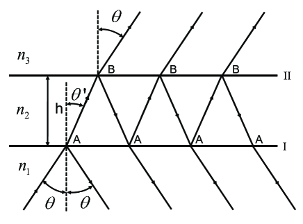
Figure 8: Wave mechanical picture of multiple reflection in a plane-parallel plate Born and Wolf (1964).

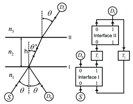
Figure 9: Left: Diagram of the experiment to measure the reflection and refraction from a plane-parallel plate. In Maxwell’s theory the source emits plane waves and the amount of energy in the reflected and transmitted light wave is recorded by detectors $D_{0}$ and $D_{1}$, respectively. Right: In the EBCM, the source emits particles which are either reflected or transmitted by the interface I. In the latter case the particle travels to interface II where it is transmitted or reflected. In the latter case the particle travels back to interface I. The time-of-flights to travel from interface I to interface II and back again are $T_{1}$ and $T_{2}$, respectively. The detectors $D_{0}$ and $D_{1}$ count the number of particles that are reflected or transmitted by the parallel plate, respectively.

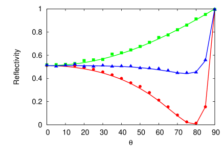
Figure 10: EBCM simulation results (markers) for the reflectivity of a parallel plate ($n_{1}=1$, $n_{2}=3$, $h=c/4fn_{2}$, $n_{3}=1.5$, corresponding to a quarter-wave plate) as a function of the angle of incidence of the incoming particles. The solid lines are the exact results of Maxwell’s theory Born and Wolf (1964). Green markers and lines: $\xi=0$ ($S$-polarization); Blue markers and lines: $\xi=\pi/4$ ($S$+$P$ polarization); Red markers and lines: $\xi=\pi/2$ ($P$-polarization). Simulation parameters: $10^{4}$ events per marker, $\gamma=\widehat{\gamma}=0.99$ and $N_{p}=1$.

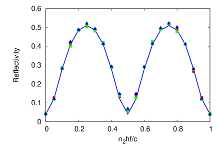
Figure 11: EBCM simulation results (markers) for the reflectivity of a parallel plate ($n_{1}=1$, $n_{3}=1.5$) as a function of the optical thickness $n_{2}hf/c$ for normal incidence of the incoming particles (see also Fig.1.18 of Ref. Born and Wolf (1964)). The solid lines are the exact results of Maxwell’s theory Born and Wolf (1964). For the legend and simulation parameters, see Fig. 10. For normal incidence, markers and solid lines for different polarizations coincide.

V.3 Two-beam interference experiments

In 1924, de Broglie introduced the idea that also matter, not just light, can exhibit wave-like properties de Broglie (1925). This idea has been confirmed in various double-slit experiments with massive objects such as electrons Jönsson (1961); Merli et al. (1976); Tonomura et al. (1989); Noel and Stroud Jr (1995), neutrons Zeilinger et al. (1988); Rauch and Werner (2000), atoms Carnal and Mlynek (1991); Keith et al. (1991) and molecules such as $C_{60}$ and $C_{70}$ Arndt et al. (1999); Brezger et al. (2002), all showing interference. In some of the double-slit experiments Merli et al. (1976); Tonomura et al. (1989); Jacques et al. (2005) the interference pattern is built up by recording individual clicks of the detectors. The intellectual challenge is to explain how the detection of individual objects that do not interact with each other can give rise to the interference patterns that are being observed. According to Feynman, the observation that the interference patterns are built up event-by-event is “impossible, absolutely impossible to explain in any classical way and has in it the heart of quantum mechanics” Feynman et al. (1965). In this section we demonstrate that this conclusion needs to be revised by constructing an EBCM for the interference experiment with two light beams that reproduces the results of Maxwell’s theory.

V.3.1 Wave theory

We consider the simple experiment sketched in Fig. 12. The sources $S_{0}$ and $S_{1}$ are lines of length $a$, separated by a center-to-center distance $d$. These sources emit coherent, monochromatic light according to a uniform current distribution, that is

$$J(x,y)=\delta(x)\left[\Theta(a/2-|y-d/2|)+\Theta(a/2-|y+d/2|)\right],$$ (65)

where $\Theta(.)$ denotes the unit step function. In the Fraunhofer regime ($d\ll X$), the light intensity at the detector on a circular screen is given by Born and Wolf (1964)

$$I(\theta)=A\left(\frac{\sin\frac{qa\sin\theta}{2}}{\frac{qa\sin\theta}{2}}\right)^{2}\cos^{2}\frac{qd\sin\theta}{2},$$ (66)

where $A$ is a constant, $q=2\pi f/c$ and $\theta$ denotes the angular position of the detector $D$ on the circular screen, see Fig. 12.

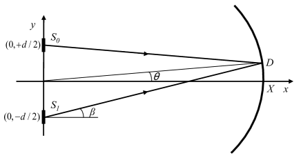
Figure 12: Schematic diagram of the double-slit experiment with two light sources $S_{0}$ and $S_{1}$ of width $a$, separated by a center-to-center distance $d$, emitting light according to a uniform current distribution (see Eq. (65)) and with a uniform angular distribution, $\beta$ denoting the angle. The light is recorded by detectors $D$ positioned on a semi-circle with radius $X$. The angular position of a detector is denoted by $\theta$.

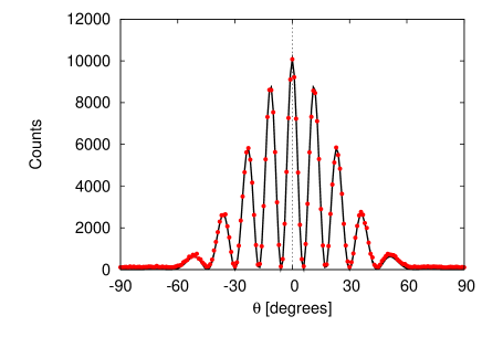
Figure 13: Detector counts (circles) as a function of the angular detector position $\theta$ as obtained from the EBCM simulation of the two-beam interference experiment depicted in Fig. 12. The solid line is a least-square fit of the EBCM data to the prediction of wave theory, Eq. (66). The sources have a width $a=c/f$ and are separated by a distance $d=5c/f$ and emit particles according to the current distribution Eq. (65). The source-detector distance $X=100c/f$, see Fig. 12. Simulation parameters: On average, each of the 181 detectors receives $10^{4}$ messengers, $\gamma=\widehat{\gamma}=0.99$ and $N_{p}=500$.

V.3.2 EBCM simulation

If it is true that individual particles build up the interference pattern one by one and that there is no direct communication between the particles, simply looking at Fig. 12 leads to the logically unescapable conclusion that the interference pattern can only be due to the internal operation of the detector Pfleegor and Mandel (1967): There is nothing else that can cause the interference pattern to appear. Of course, the EBCM of a detector is designed to cope with this task.

In the EBCM, the messengers leave the source one-by-one, at positions $y$ drawn randomly from a uniform distribution over the interval $[-d/2-a/2,-d/2+a/2]\cup[+d/2-a/2,+d/2+a/2]$, see Eq. (65). The angle $\beta$ is a uniform pseudo-random number between $-\pi/2$ and $\pi/2$. When a messenger is created, its time-of-flight is set to zero. For simplicity, we consider the case of fully polarized light (the same $\xi$ for all messagers) only.

When a messenger travels from the source at $(0,y)$ to the circular detector screen with radius $X$, it updates its own time-of-flight. Specifically, a messenger leaving the source at $(0,y)$ under an angle $\beta$ (see Fig. 12) will hit the detector screen at a position determined by the angle $\theta$ given by

$$\sin\theta=\frac{y\cos^{2}\beta+\sin\beta\sqrt{X^{2}-y^{2}\cos^{2}\beta}}{X},$$ (67)

where $|y/X|<1$. The time-of-flight $t$ is then given by

$$t=\frac{\sqrt{X^{2}-2yX\sin\theta+y^{2}}}{c}.$$ (68)

As a messenger hits a detector, this detector updates its internal state (the internal states of all other detectors do not change) using the data contained in the message and then decides whether to generate a zero or a one output event. Only after the messenger has been processed by the detector, the source is allowed to emit a new messenger. This process is then repeated many times.

In Fig. 13, we present simulation results for a representative case. A Mathematica implementation that uses a variant Jin et al. (2010a) of the EBCM used in this paper can be downloaded from the Wolfram Demonstration Project web site DS .

From Fig. 13 it is clear that the EBCM reproduces the results of Maxwell’s theory without taking recourse of the solution of a wave equation and that the detection efficiency of the detectors is very close to 100%. In other words, the interference patterns generated by EBCM cannot be attributed to ineffecient detectors.

V.4 Remarks

It is of interest to compare the detection counts, observed in the EBCM simulation of the two-beam interference experiment, with those observed in a real experiment with single photons Jacques et al. (2005). In the simulation that yields the results of Fig. 13, each of the 181 detectors making up the detection area is hit on average by ten thousand photons and the total number number of clicks generated by the detectors is 296444. Hence, the ratio of the total number of detected to emitted photons is of the order of 0.16, orders of magnitude larger than the ratio $0.5\times 10^{-3}$ observed in the single-photon interference experiments Jacques et al. (2005).

VI Optical Components

The EBCM of optical components such as wave plates and beam splitters can be constructed by connecting several units that simulate the interfaces (with suitable parameters) of these components Trieu et al. (2010). From a simulation point of view, such a construction is both inefficient and unnecessary. Having shown that two connected EBCM’s of an interface reproduce the result of a plane parallel plate, it is legitimate to replace the two interfaces by one “lumped” EBCM that simulates a beam splitter for instance Trieu et al. (2010). In this section, we specificy the lumped EBCM of optical components that are used in quantum optics experiments.

VI.1 Beam splitter

The processing unit that acts as a beam splitter (BS) has the generic structure, depicted in Fig. 4. The device has two input and two output ports labeled by $k=0,1$ and consists of an input stage, a DLM, a transformation stage (T), and an output stage (O) De Raedt et al. (2005a, b, c); Michielsen et al. (2005). In fact, up to the transformation matrix $\mathbf{T}$, the processing unit is identical to the one of a single interface.

For a 50-50 BS, the transformation matrix $\mathbf{T}$ reads

$$\mathbf{T}=\frac{1}{\sqrt{2}}\left(\begin{array}[]{lccr}1&i&0&0\\ i&1&0&0\\ 0&0&1&i\\ 0&0&i&1\end{array}\right),$$ (69)

which is the same as the one employed in wave theory.

VI.2 Polarizing Beam Splitter

A polarizing beam splitter (PBS) is used to redirect the photons depending on their polarization. For simplicity, we assume that the coordinate system used to define the incoming messages coincides with the coordinate system defined by two orthogonal directions of polarization of the PBS.

The processing unit that acts as a PBS has the generic structure depicted in Fig. 4. The unit differs from the previous ones in the details of the transformation matrix $\mathbf{T}$ only. For instance, if the PBS passes $S$-polarized light, it reflects $P$-polarized light. In this case, the transformation matrix $\mathbf{T}$ of a PBS reads

$$\mathbf{T}=\left(\begin{array}[]{lccr}1&0&0&0\\ 0&1&0&0\\ 0&0&0&i\\ 0&0&i&0\end{array}\right),$$ (70)

which is the same as the one employed in wave theory.

VI.3 Wave plates

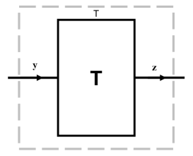
Figure 14: Diagram of a processing unit that performs an event-based simulation of wave plates. Compared to the generic diagram Fig. 4, the DLM stage and the output stage are missing. The solid lines represent the input and output ports of the device. The presence of a message is indicated by an arrow on the corresponding port line. The transformation matrices ${\bf T}$ for the HWP and QWP are given by Eq. (71) and Eq. (72), respectively.

A half-wave plate (HWP) changes the polarization of the light but also changes its phase. A quarter-wave plate (QWP) changes the polarization of the light and induces a phase difference between the $S$ and $P$ components. In optics, both plates are often used as retarders. In the EBCM, this retardation of the wave corresponds to a change in the time-of-flight of the messenger.

In contrast to the BS and PBS, as lumped devices the HWP and QWP may be simulated without the input stage, that is the DLM may be omitted. The lumped device has only one input and one output port, as shown in Fig. 14, and we therefore omit the subscript that labels that input and output port in the following.

The transformation performed by the HWP reads

$$\mathbf{T}=-i\left(\begin{array}[]{lr}\cos 2\theta&\sin 2\theta\\ \sin 2\theta&-\cos 2\theta\end{array}\right),$$ (71)

where $\theta$ denotes the angle of the optical axis with respect to the laboratory frame. Similarly, the transformation performed by the QWP is

$$\mathbf{T}=\frac{1}{\sqrt{2}}\left(\begin{array}[]{lr}1-i\cos 2\theta&-i\sin 2\theta\\ -i\sin 2\theta&1+i\cos 2\theta\end{array}\right).$$ (72)

VI.4 Ideal mirror

The EBCM model of an interface with $\widetilde{r}_{S}=\widetilde{r}_{P}=1$ can be used to simulate the operation of an ideal mirror but from a computational viewpoint, it is both inefficient and unnecessary to simulate the ideal mirror in this manner. An ideal mirror merely acts as a hard wall at which the messengers undergo an elastic scattering event and the second component of the message $\mathbf{y}$ changes sign. In practice, these rules are trivial to implement in a simulation.

VII Single-photon quantum optics experiments

In the EBCM approach, the processing units that simulate the optical components are connected in such a way that the simulation setup is an exact one-to-one copy of the laboratory experiment. The source sends messengers one-by-one but at all times, there is at most one messengers being routed through the network of processing units. Only after a detector has processed the messenger, the source is allowed to create a new messenger. This procedure guarantuees that the simulation process trivially satisfies Einstein’s criterion of local causality. Needless to say, the internal state of the processors may be given an interpretation in terms of the polarization, displacement or any other classical concept that describes the state of the material (atoms, molecules…). In other words, all the elements of the EBCM may be given an interpretation within the realm of classical physics. As any such interpretation, which would be necessarily subjective, has no impact on the facts produced by the EBCM, we will not engage in the endeavour to give such an interpretation.

VII.1 Mach-Zehnder interferometer

A description of the MZI was given in Section II. In Fig. 15, we present the EBCM simulation results for the number of particles registered by detectors $D_{0}$ and $D_{1}$, divided by the total count of detected particles, as a function of the difference between the time-of-flight in the lower and upper arm of the MZI, respectively. In this simulation, we set $T_{1}(x)=T_{0}-2\pi x/f$ such that $f\Delta T=f(T_{0}-T_{1}(x))=2\pi x$ and vary $x$ from zero to one. From Fig. 15, it is clear that the EBCM model reproduces the results of Maxwell’s theory.

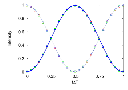
Figure 15: EBCM simulation results for the number of particles registered by detectors $D_{0}$ (solid markers) and $D_{1}$ (open markers), divided by the total count of detected particles, as a function of the difference $\Delta T=(T_{0}-T_{1}(x))$ between the time-of-flight in the lower and upper arm of the MZI, respectively. The solid and dashed lines are the exact results of Maxwell’s theory for the normalized intensities at $D_{0}$ and $D_{1}$, respectively. Simulation parameters: $10^{4}$ events per pair of open en closed markers, $\gamma=\widehat{\gamma}=0.99$. The markers for different polarizations (for the legend, see Fig. 10) coincide, in agreement with Maxwell’s theory.

The MZI may well be the simplest example that illustrates the conceptual difficulties that arise when one tries to apply concepts of quantum theory to give a rational, logically consistent, explanation of what actually happens to the photons in the MZI. As shown in the experiment of Grangier et al Grangier et al. (1986), photons may be considered as indivisable particles Garrison and Chiao (2009), each one following one particular path through the MZI. Assuming that the observed interference in this experiment can only be a wave phenomenon, the somewhat mystical concept of wave-particle duality is introduced. It is said that photons exhibit both wave and particle behavior depending upon the circumstances of the experiment Home (1997), in contradiction with the experiment Grangier et al. (1986) which shows that photons are indivisable particles. As a last resort to save the quantum theoretical explanation, another mystical element, namely the collapse of the wave function is introduced. The collapse mechanism has remained mystical after hunderd years of using quantum theory: A logically and physically acceptable, experimentally testable mechanism has not been found. In effect, the main purpose of these two mystical elements is to demonstrate, what is long known, that quantum theory does not provide any insight into what happens in the system. It does not contain the elements to give a cause-and-effect description of natural phenomena but describes the statistical properties of our observations very well. Instead of searching for rational cause-and-effect descriptions, to get out of the logical mess created by introducing elements of magic, quantum theory simply postulates that such a rational cause-and-effect description does not exist.

In the EBCM approach, there is no need to invoke elements of magic or irrational reasoning to explain the results of the MZI experiment of Grangier et al Grangier et al. (1986). The crux is that realize that interference is not necessarily a wave phenomenon but can be generated by particles that interact with some agent (the processors in the EBCM).

VII.2 Wheeler’s delayed choice experiment

In 1978, Wheeler proposed a gedanken experiment Wheeler , a variation on Young’s double slit experiment, in which the decision to observe wave or particle behavior is made after the photon has passed the slits. The pictorial description of this experiment defies common sense: The behavior of the photon in the past is said to be changing from a particle to a wave or vice versa.

VII.2.1 Experiment

In an experimental realization of Wheeler’s delayed choice experiment, Jacques et al. Jacques et al. (2007) send linearly polarized single photons through a polarizing beam splitter (PBS) that together with a second, movable PBS forms an interferometer (see Fig. 16). Moving the second PBS induces a time-delay in one of the arms of the interferometer Jacques et al. (2007), symbolically represented by $T_{1}(x)$ in Fig. 16. The electro-optic modelator (EOM) performs the same function as a HWP. Changing the electrical potential applied to the EOM, changes the rotational angle that mixes the two polarizations, see Eq. (71). In the experiment Jacques et al. (2007), the random number generator RNG generates a sequence of binary random numbers $r_{n}=0,1$. The output of RNG is used to control the potential applied to the EOM. If $r_{n}=0$, the rotation angle $\theta_{\mathrm{EOM}}=0$ and if $r_{1}$, $\theta_{\mathrm{EOM}}=\pi/8$. In the former case, there can be no interference: There is no mixing of $S$- and $P$-polarized light. In the latter case, interference can occur and we expect an interference pattern that is the same as the one of a MZI.

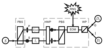
Figure 16: Schematic diagram of the experimental setup for Wheeler’s delayed-choice experiment with single photons Jacques et al. (2007). EOM: electro-optic modulator; RNG: Random number generator; WP: Wollaston prism (= PBS); $D_{0}$, $D_{1}$: Detectors. The EBCM replaces the physical devices by the corresponding message-processing units.

Detector $D_{0}$ ($D_{1}$) counts the events generated at port 0 (1) of the Wollaston prism (WP). During a run of $N$ events, the algorithm generates the data set

$$\Gamma=\left\{d_{n},r_{n}|n=1,...,N;f\Delta T\right\},$$ (73)

where $d_{n}=0$ ($1$) indicates that detector $D_{0}$ ($D_{1}$) fired and $r_{n}=0,1$ is a binary pseudo-random number that is chosen after the $n$th message has passed the first PBS.

VII.2.2 EBCM simulation

We simulate the Wheeler delayed-choice experiment of Fig. 16 by connecting the various EBCM of the optical components in exactly the same manner as in Fig. 16. The simulation generates the data set $\Gamma$ just like in the experiment Jacques et al. (2008, 2007) and is analyzed in the same manner. The EBCM simulation results presented in Fig. 17 show that there is excellent agreement between the event-based simulation data and the predictions of wave theory.

Of course, in the case of the classical, locally causal EBCM, there is no need to resort to concepts such as particle-wave duality and the mysteries of delayed-choice to give a rational explanation of the observed phenomena. In the simulation we can always track the particles, independent of $r_{n}=0,1$. These particals always have full which-way information, never directly communicate with each other, arrive one by one at a detector but nevertheless build up an interference pattern at the detector if $r_{n}=1$. Thus, the EBCM of Wheeler’s delayed-choice experiment provides a unified particle-only description of both cases $r_{n}=0,1$ that does not defy common sense.

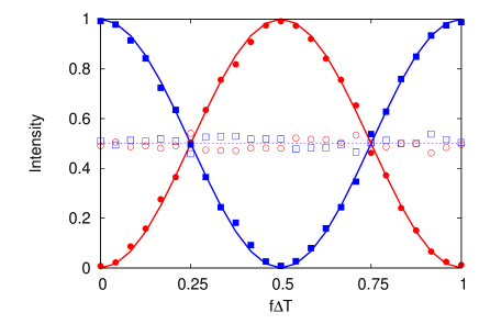
Figure 17: EBCM simulation results (markers) for the Wheeler delayed-choice experiment depicted in Fig. 16. The number of particles registered by detectors $D_{0}$ and $D_{1}$ divided by the total count of detected particles, as a function of the difference $\Delta T=(T_{0}-T_{1}(x))$ between the time-of-flight in the lower and upper arm of the interferometer, respectively. Open circles: Intensity measured by $D_{0}$ for $\theta_{\mathrm{EOM}}=0$ ($r_{n}=0$); Open squares: Intensity measured by $D_{1}$ for $\theta_{\mathrm{EOM}}=0$; Closed circles: Intensity measured by $D_{0}$ for $\theta_{\mathrm{EOM}}=\pi/4$ ($r_{n}=1$); Closed squares: Intensity measured by $D_{1}$ for $\theta_{\mathrm{EOM}}=\pi/4$; Dashed line: Intensities measured by $D_{0}$ and $D_{1}$ as obtained from Maxwell’s theory for $\theta_{\mathrm{EOM}}=0$; Solid red (blue) line: Intensity measured by $D_{0}$ ($D_{1}$) as obtained from Maxwell’s theory for $\theta_{\mathrm{EOM}}=\pi/4$. Simulation parameters: $2600$ emitted events per pair of open/closed markers, $\gamma=\widehat{\gamma}=0.99$ and $N_{p}=1$. The actual counts ($=1300\times\mathrm{intensities}$) are in good quantitative agreement with the experimental results reported in Ref. Jacques et al. (2007).

VII.3 Quantum Eraser

In 1982, Scully and Drühl proposed a photon interference experiment, called “quantum eraser” Scully and Drühl (1982), in which the photons are labelled by which-way markers. In this experiment, the which-way information of the photons is known to the experimenter and hence, according to common lore, no interference is to be expected. However by erasing the which-way information afterwards by a “quantum eraser”, the interference pattern can be recovered Scully and Drühl (1982), even from data that has been recorded and saved in a file Kim et al. (2000).

Quantum eraser experiments have been described “as one of the most intriguing effects in quantum mechanics”, but have also been regarded as “the fallacy of delayed choice and quantum eraser” Aharonov and Zubairy (2005). Clearly, they challenge the point of view that the wave and particle behavior of photons are complementary: The observation of interference, commonly associated with wave behavior, depends on the way the data is analyzed after the photons have passed through the interferometer.

The quantum eraser has been implemented in several different experiments with photons, atoms, etc. Scully et al. (1991); Kwiat et al. (1992); Pittman et al. (1996); Schwindt et al. (1999); Kim et al. (2000); Walborn et al. (2002); Scarcelli et al. (2007). In this paper, we consider the experiment performed by Schwindt et al. Schwindt et al. (1999) in which the polarization of the photons is employed to encode the which-way information. The experimental setup (see Fig. 18) consists of a linearly polarized single-photon source (not shown), a MZI of which the time-of-flight of path 1 (see Fig. 18) can be varied by moving the mirror $M$ and an analysis system which is a combination of a QWP, a HWP (HWP1), and a calcite prism (WP) operating as a PBS. Another adjustable HWP (HWP0) is inserted in path 0 of the MZI to entangle the photon’s path with its polarization Schwindt et al. (1999).

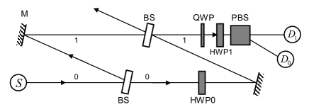
Figure 18: Schematic diagram of the experimental setup for the quantum eraser experiment with photons studied in Ref. Schwindt et al. (1999). Moving the mirror labeled M changes the difference $\Delta T$ between the time-of-flight in the lower and upper arm of the interferometer.

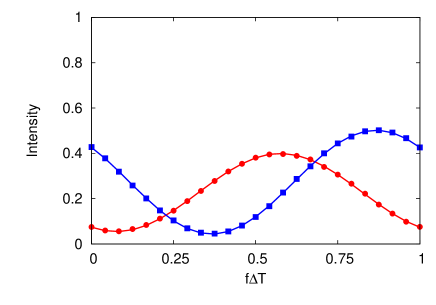
Figure 19: The number of particles registered by detectors $D_{0}$ and $D_{1}$ divided by the total count of detected particles as a function of the time-of-flight difference $\Delta T$ for $\theta_{0}=\pi/3$, $\theta_{1}=\pi/4$, and $\theta_{2}=\pi/8$, as obtained from the EBCM simulation of the quantum eraser experiment depicted in Fig. 18. Circles: Intensity measured by $D_{0}$; Squares: Intensity measured by $D_{1}$; Solid red (blue) line: Intensity measured by $D_{0}$ ($D_{1}$) as obtained from Maxwell’s theory, see Eq. (75). Simulation parameters: $10^{4}$ events, $\gamma=\widehat{\gamma}=0.99$ and $N_{p}=1$.

VII.3.1 Wave theory

If a photon, described by a pure $S$-polarized state is injected into the interferometer with the HWP0 set to $45^{\circ}$, the photon that arrives at the second BS of the MZI carries a which-way marker: The photon will be in the $P$ polarized state if it followed path 0 and will be in the $S$ polarized state if it followed path 1. If the rotation angle of HWP1 is zero, there will be no interference and the detectors reveal the full which-way information of each detected photon. If the rotation angle of HWP1 is nonzero, the $S$- and $P$-polarized states interfere, the which-way information of each photon will be partially or completely “erased”. Thus, by varying the rotation angle of HWP1, the illusion is created that the character of the photon in the MZI “changes” from particle to wave and vice versa.

Assuming that the photons emitted by the source are described by a pure $S$-polarized state, wave theory predicts that the intensities at the detectors $D_{0}$ and $D_{1}$ are given by

$$I_{0} = \frac{1}{16}\left\{4-\cos 4(\theta_{2}-\theta_{1})-\cos 4\theta_{1}\right.$$ (74)

$$\left.-\cos 4(\theta_{2}-\theta_{1}-\theta_{0})-\cos 4(\theta_{1}-\theta_{0})\right.$$

$$\left.+4\cos f\Delta T\sin(2\theta_{2}-4\theta_{1})\sin 2\theta_{0}\right.$$

$$\left.-2\sin f\Delta T[\cos(4\theta_{2}-4\theta_{1}-2\theta_{0})\right.$$

$$\left.+\cos(4\theta_{1}-2\theta_{0})-2\cos 2\theta_{0}]\right\}$$

$$I_{1} = \frac{1}{16}\left\{4+\cos 4(\theta_{2}-\theta_{1})+\cos 4\theta_{2}\right.$$ (75)

$$\left.+\cos 4(\theta_{2}-\theta_{1}-\theta_{0})+\cos 4(\theta_{1}-\theta_{0})\right.$$

$$\left.-4\cos f\Delta T\sin(2\theta_{2}-4\theta_{1})\sin 2\theta_{0}\right.$$

$$\left.+2\sin f\Delta T[\cos(4\theta_{2}-4\theta_{1}-2\theta_{0})\right.$$

$$\left.+\cos(4\theta_{1}-2\theta_{0})+2\cos 2\theta_{0}]\right\},$$

where $\theta_{0}$, $\theta_{1}$, and $\theta_{2}$ are the rotation angles of HWP0, HWP1, and QWP, respectively.

VII.3.2 EBCM simulation

In an earlier paper in this journal, it was shown that quantum eraser experiments can be simulated without invoking concepts of quantum theory and without first solving a wave mechanical problem Jin et al. (2010b). In this paper, we demonstrate that the same experiment can be simulated by simply re-using the EBCM of the optical components.

In Fig. 19 we present the results of an event-by-event simulation of the experiment depicted in Fig. 18. It is clear that there is excellent agreement between the EBCM data and the prediction of quantum theory for the system described by the pure state. Elsewhere, we have already demonstrated that the EBCM can also cope with systems that quantum theory describes in terms of mixed states Jin et al. (2010b). The EBCM correctly describes the outcome of the quantum eraser experiment of Fig. 18 under all circumstances Jin et al. (2010b).

VII.4 Single-photon tunneling

A conceptually simple, direct experimental demonstration that photons behave as indivisable entities and that displays both particle and wave characteristics was proposed by Ghose et al. Ghose et al. (1991), drawing inspiration from an experiment that was carried out with microwaves almost hundred years earlier Bose (1897). The experimental setup is sketched in Fig. 20.

It is instructive to consider Maxwell’s theory for this experiment first. A light wave is sent to a prism that is separated from another prism by a distance $w$. If $w$ is very large, the total internal reflection in the first prism causes virtually all light to be reflected Born and Wolf (1964). If $w$ is of the order of the wavelength or less, evanescent waves at the surface of the first prism can penetrate the second prism, giving rise to a measurable flux of light in the second prism Bose (1897). It is said that the wave can “tunnel” through the gap separating the prisms. In the case of waves, the experimental observation of this tunneling effect can be completely understood within the framework of Maxwell’s theory.

Let us now try to explain this observation if we accept, as we do in this paper, that light is made out of indivisable entities, that is out of photons. Assuming ideal single-photon detectors and a single-photon source, the experiment may show that

1. Both detectors $D_{0}$ and $D_{1}$ click within a time window, much smaller than the time between two successive single-photon emissions.

2. Detectors $D_{0}$ and $D_{1}$ click in perfect anti-coincidence.

Experimental results favor possibility (2) Mizobuchi and Ohtaké (1992); Unnikrishnan and Murthy (1996); Brida et al. (2004) (see also our discussion of the experiment by Grangier et al. in Section I.1) and within the standard interpretation of quantum theory are considered to be a proof that the particle-wave duality must be considered in weak sense and not in the orginal “complementarity” sense of Bohr Home (1997); Brida et al. (2004). There is not much point to dwell on this issue here because, as we show now, the EBCM approach provides a simple picture of this phenomenon without introducing the mystique of particle-wave duality.

The results of an EBCM simulation, using the “lumped device” representation of the two-prism system, of the experiment depicted in Fig. 20 are shown in Fig. 21, together with the predictions of Maxwell’s theory. It is clear that there is excellent agreement between the corpuscular model and the wave model, demonstrating once more that the predictions of the latter can be obtained from a simulation that involves particles only.

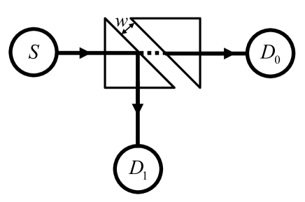
Figure 20: Schematic diagram of the experimental setup for the photon tunneling experiment Ref. Mizobuchi and Ohtaké (1992). The hypotenuses of the identical prisms are separated from each other by a distance $w$.

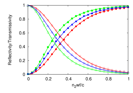
Figure 21: The number of particles registered by detectors $D_{0}$ (transmissivity, open markers) and $D_{1}$ (reflectivity, closed markers) divided by the total count of detected particles as a function of the width $w$ of the gap between the two prisms ($n=1.52$), as obtained from an EBCM simulation of the photon tunneling experiment depicted in Fig. 20. The solid lines are the exact results of Maxwell’s theory Born and Wolf (1964). Green markers and lines: $\xi=0$ ($S$-polarization); Blue markers and lines: $\xi=\pi/4$ ($S$+$P$ polarization); Red markers and lines: $\xi=\pi/2$ ($P$-polarization). Simulation parameters: $10^{4}$ events per marker, $\gamma=\widehat{\gamma}=0.99$ and $N_{p}=1$.

VIII Photon correlation experiments

VIII.1 Einstein-Podolsky-Rosen-Bohm experiment

To construct an event-based computer simulation model of the EPRB experiment with photons performed by Weihs et al. Weihs et al. (1998)), we use the same EBCMs for the optical components as in the previous sections. The resulting EBCM for the whole EPRB experiment is substantially different from our earlier event-based simulation models that reproduce the result of quantum theory for the singlet state and product state De Raedt et al. (2006a, 2007a, 2007b, 2007c, 2007d); Zhao et al. (2008b). The difference is that in our earlier work we adpoted the tradition in this particular subfield to use simplified mathematical models for the optical components that, when re-used for different optics experimements, would fail to reproduce the results of these experiments. In this section, we simply use (without any modification) the EBCMs for the optical components that are present in the laboratory experiment and analyze the simulation data in exactly the same manner as the experimental data for this experiment has been analyzed Weihs et al. (1998).

VIII.1.1 Laboratory experiment

In Fig. 22, we show a schematic diagram of an EPRB experiment with photons (see also Fig. 2 in Weihs et al. (1998)). The source emits pairs of photons. Each photon of a pair travels to an observation station in which it is manipulated and detected. The two stations are assumed to be identical. They are separated spatially and temporally, preventing the observation at station 1 (2) to have a causal effect on the data registered at station $2$ (1) Weihs et al. (1998). As the photon arrives at station $i=1,2$, it passes through an EOM that rotates the polarization of the photon by an angle depending on the voltage applied to the modulator. These voltages are controlled by two independent binary random number generators. A PBS sends the photon to one of the two detectors. The station’s clock assigns a time-tag to each generated signal. We consider two different experiments, one in which the source emits photons with opposite but otherwise unpredictable polarization and those with a source emitting photons with fixed polarization.

VIII.1.2 Quantum theory

The quantum theoretical description of the EPRB experiment with photons exploits the fact that the two-dimensional vector space spanned by two orthogonal polarization vectors is isomorphic to the vector space of spin-1/2 particles. The predictions of quantum theory  for the single and two-particle averages for an experiment described by a quantum system of two spin-1/2 particles in the singlet state and a product state are given in Table 1 and serve as a reference for the EBCM simulation.

Table 1: The single spin expectations, the two-spin expectation and the spin-spin correlation of two spin-1/2 particles in the singlet state $|\mathrm{Singlet}\rangle=\left({|{SP}\rangle-|{PS}\rangle}\right)/\sqrt{2}$ and in the product state $|\mathrm{Product}\rangle=(\cos\eta_{1}|P\rangle_{1}+\sin\eta_{1}|S\rangle_{1})(\cos\eta_{2}|P\rangle_{2}+\sin\eta_{2}|S\rangle_{2})$.

	$|\mathrm{Singlet}\rangle$	$|\mathrm{Product}\rangle$
$\widehat{E}_{1}(\alpha_{1})$	$0$	$\cos 2(\alpha_{1}-\eta_{1})$
$\widehat{E}_{2}(\alpha_{2})$	$0$	$\cos 2(\alpha_{2}-\eta_{2})$
$\widehat{E}_{12}(\alpha_{1},\alpha_{2})$	$-\cos 2(\alpha_{1}-\alpha_{2})$	$\cos 2(\alpha_{1}-\eta_{1})\cos 2(\alpha_{2}-\eta_{2})$
$\widehat{\rho}_{12}(\alpha_{1},\alpha_{2})$	$\widehat{E}_{12}(\alpha_{1},\alpha_{2})$	0

VIII.1.3 EBCM of the EPRB experiment

The detectors, PBSs and EOMs are simulated using their EBCMs described earlier. Recall that the EBCM of the detector mimics a detector with 100% detection efficiency. The EBCM of the EPRB experiment trivially satisfies Einstein s criteria of local causality, does not rely on any concept of quantum theory and, as will be shown below, reproduces the results of quantum theory for both types of experiments.

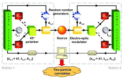
Figure 22: Schematic diagram of an EPRB experiment with photons Weihs et al. (1998).

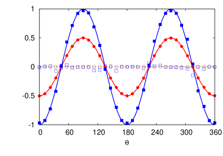
Figure 23: Computer simulation data and quantum theoretical results for the single-particle and two-particle averages of the EPRB experiment depicted in Fig. 22 as a function of $\theta=\alpha_{1}-\alpha_{2}$. The source emits particles with opposite polarization, uniformly distributed over the unit circle. Open circles and squares: Eq. (79) and 79), respectively; Closed squares: Eq. (80) Closed circles: Eq. (81) for $W=T_{\mathrm{EPRB}}$, that is by ignoring the time-tag data; Blue solid line: $\widehat{E}_{12}(\alpha_{1},\alpha_{2})=-\cos 2\theta$; Red solid line: $-2^{-1}\cos 2\theta$. Simulation parameters: $3\times 10^{5}$ pairs, $T_{\mathbf{EPRB}}=1000$, $W=1$, $d=4$, $\gamma=\widehat{\gamma}=0.99$ and $N_{p}=1$. Note that the total number of pairs emitted by the source is about the same as the number of photons per station detected in the experiment reported in Ref. Weihs et al. (1998) (experimental data set called longdist35).

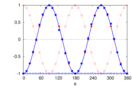
Figure 24: Computer simulation data and quantum theoretical results for the single-particle and two-particle averages of the EPRB experiment depicted in Fig. 22 as a function of $\theta=\alpha_{1}-\eta_{1}$ with $\alpha_{2}=0$. Same as in Fig. 23 except that the source emits particles with with $P$ ($\eta_{1}=0$) and $S$ ($\eta_{2}=\pi/2$) polarization only. Open circles and squares: Eq. (79) and 79), respectively; Closed squares: Eq. (80) Closed circles: Eq. (81) for $W=T_{\mathrm{EPRB}}$, that is by ignoring the time-tag data; Blue solid line: $\widehat{E}_{12}(\alpha_{1},\alpha_{2})=\cos 2(\alpha_{1}-\eta_{1})\cos 2(\alpha_{2}-\eta_{2})=-\cos 2\theta$. Simulation parameters: Same as in Fig. 23.

The data generated by the EBCM of the EPRB experiment is analyzed in exactly the same manner as in experiment Weihs et al. (1998). In the simulation, the firing of a detector is regarded as an event. At the $n$th event, the data recorded on a hard disk at station $i=1,2$ consists of $x_{n,i}=\pm 1$, specifying which of the two detectors fired, the time tag $t_{n,i}$ indicating the time at which a detector fired, and the two-dimensional unit vector $\alpha_{n,i}$ that represents the rotation of the polarization by the EOM at the time of detection. Hence, the set of data collected at station $i=1,2$ during a run of $N$ events may be written as

$$\Upsilon_{i}=\left\{{x_{n,i}=\pm 1,t_{n,i},\alpha_{n,i}|n=1,\ldots,N}\right\}.$$ (76)

In the (computer) experiment, the data $\{\Upsilon_{1},\Upsilon_{2}\}$ may be analyzed long after the data has been collected Weihs et al. (1998). Coincidences are identified by comparing the time differences $\{t_{n,1}-t_{n,2}|n=1,\ldots,N\}$ with a time window Weihs et al. (1998) $W$. Introducing the symbol $\sum^{\prime}$ to indicate that the sum has to be taken over all events that satisfy $\alpha_{i}=\alpha_{n,i}$ for $i=1,2$, for each pair of directions $\alpha_{1}$ and $\alpha_{2}$ of the EOMs, the number of coincidences $C_{xy}\equiv C_{xy}(\alpha_{1},\alpha_{2})$ between detectors $D_{x,1}$ ($x=\pm 1$) at station 1 and detectors $D_{y,2}$ ($y=\pm 1$) at station 2 is given by

$$C_{xy} = \mathop{{\sum}^{\prime}}_{n=1}^{N}\delta_{x,x_{n,1}}\delta_{y,x_{n,2}}\Theta(W-|t_{n,1}-t_{n,2}|),$$ (77)

where $\Theta(t)$ is the Heaviside step function. We emphasize that we count all events that, according to the same criterion as the one employed in experiment, correspond to the detection of pairs Weihs et al. (1998). The average single-particle counts are defined by

$$E_{1}(\alpha_{1},\alpha_{2})=\frac{\sum_{x,y=\pm 1}xC_{xy}}{\sum_{x,y=\pm 1}C_{xy}},$$ (78)

and

$$E_{2}(\alpha_{1},\alpha_{2})=\frac{\sum_{x,y=\pm 1}yC_{xy}}{\sum_{x,y=\pm 1}C_{xy}},$$ (79)

where the denominator is the sum of all coincidences.

The correlation of two dichotomic variables $x$ and $y$ is defined by Grimmet and Stirzaker (1995)

$$\rho_{12}(\alpha_{1},\alpha_{2})=E_{12}(\alpha_{1},\alpha_{2})-E_{1}(\alpha_{1},\alpha_{2})E_{2}(\alpha_{1},\alpha_{2}),$$ (80)

where

$$E_{12}(\alpha_{1},\alpha_{2}) = \frac{\sum_{x,y}xyC_{xy}}{\sum_{x,y}C_{xy}}$$ (81)

$$= \frac{C_{++}+C_{--}-C_{+-}-C_{-+}}{C_{++}+C_{--}+C_{+-}+C_{-+}},$$

is the two-particle average.

In general, the values for the average single-particle counts $E_{1}(\alpha_{1},\alpha_{2})$ and $E_{2}(\alpha_{1},\alpha_{2})$, the two-particle averages $E(\alpha_{1},\alpha_{2})$, and the total number of the coincidences $C(\alpha_{1},\alpha_{2})=\sum_{x,y=\pm 1}C_{xy}(\alpha_{1},\alpha_{2})$, not only depend on the directions $\alpha_{1}$ and $\alpha_{2}$ but also on the time window $W$ used to identify the coincidences.

VIII.1.4 Time-tag model

From Eq. (76), it is clear that a model that aims to describe real EPRB experiments should incorporate a mechanism to produce the time tags $t_{n,1}$ and $t_{n,2}$. The importance of incorporating such a mechanism has been pointed out by S. Pascazio who presented a concrete time-tag model that yields a good approximation to the correlation of the singlet state (see Table 1) Pascazio (1986).

Following our earlier work De Raedt et al. (2006a, 2007b, 2007a, 2007c, 2007d), we assume that as a particle passes through the EOM, it experiences a time delay. This is a very reasonable assumption as EOMs are in fact used as retarders in optical communication systems. For simplicity, the time delay ${t}_{n,i}$ is assumed to be distributed uniformly over the interval $[0,T]$. From our earlier work we know that the choice $T=T_{\mathbf{EPRB}}\sin^{2d}2(\xi_{n}-\alpha_{n,i})$ rigorously reproduces the results of Table 1, that is the results of quantum theory for the EPRB experiment, if $d=4$ and $W\ll T_{\mathbf{EPRB}}$ De Raedt et al. (2006a, 2007b, 2007a, 2007c, 2007d). Therefore, we adopt this time-tag model in the present paper also.

VIII.1.5 Simulation results

The EBCM generates the data set Eq. (76), just as experiment does Weihs et al. (1998). We choose the coincidence window $W$ and compute the coincidences, single-spin and two-spin averages according to the Eqs. (77)–(81). The simulation results for the two different types of experiments are presented in Figs. 23 and 24. It is obvious that the fully classical, locally causal EBCM reproduces the results of quantum theory  for both the singlet state and the product state. Note that the detectors have 100% detection efficiency.

VIII.1.6 Remarks

It is not uncommon to find in the literature, statements that it is impossible to simulate quantum phenomena by classical processes. Such statements are thought to be a direct consequence of Bell’s theorem Bell (1993) but are in conflict with other work that has pointed out the irrelevance of Bell’s theorem  de la Peña et al. (1972); Fine (1974, 1982a, 1982b, 1982c); de Muynck (1986); Jaynes (1989); Brody (1993); Fine (1996); Khrennikov (1999); Sica (1999); De Baere et al. (1999); Hess and Philipp (2001, 2005); Accardi (2005); Kracklauer (2005); Santos (2005); Morgan (2006); Khrennikov (2007); Adenier and Khrennikov (2007); Nieuwenhuizen (2009); Matzkin (2009); De Raedt et al. . This conclusion is supported by several explicit examples that prove that it is possible to construct algorithms that satisfy Einstein’s criteria for locality and causality, yet reproduce exactly the two-particle correlations of a quantum system in the singlet state, without invoking any concept of quantum theory De Raedt et al. (2006a, 2007a, 2007b, 2007c, 2007d); Zhao et al. (2008a). The simulation results presented in Fig. 23, obtained from different (but similar) simulation models than the ones used in previous work, provides yet another illustration that Bell’s no-go theorem is of very limited value: It applies to a marginal class of classical models only and becomes relevant to the EPRB experiments that are performed in the laboratory if the coincidence window $W$ approaches infinity (on the time scale of the experiment).

VIII.2 Hanbury Brown-Twiss experiment

HBT experiments Brown and Twiss (1956) measure the correlation of light intensities orginating from two different, uncorrelated sources. HBT showed that under conditions for which the usual two-beam interference fringes measured by each of the two detectors vanish, the correlated intensities of the two detectors can still show interference fringes. When a HBT experiment is performed with detectors operating in the single-photon-detection regime, the observation of the fringes in the correlated detector intensities is attributed to the wave-particle duality of the beam Glauber (1963a, b); Mandel (1999).

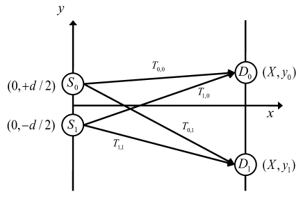
Figure 25: Schematic diagram of a HBT experiment. Single photons emitted from point sources $S_{0}$ and $S_{1}$ are registered by two detectors $D_{0}$ and $D_{1}$. The time-of-flight for each of the four possible paths from source $S_{m}$ to detector $D_{n}$ is denoted by $T_{m,n}$ where $m,n=0,1$.

VIII.2.1 Scalar wave theory

Conceptually, the HBT experiment of Fig. 25 can be viewed as a two-beam experiment with two detectors. Assume that source $S_{m}$ ($m=0,1$) emits coherent light of frequency $f$ and produces a wave with amplitude $A_{m}e^{i\phi_{m}}$ ($A_{m}$ and $\phi_{m}$ real). For simplicity of presentation, we assume that $A_{0}=A_{1}=A$. According to Maxwell’s theory, the total wave amplitude $B_{n}$ on detector $n$ is

$$B_{n}=A\left(e^{i(\phi_{0}+2\pi fT_{0,n})}+e^{i(\phi_{1}+2\pi fT_{1,n})}\right),$$ (82)

where the time-of-flight for each of the four possible paths from source $S_{m}$ to detector $D_{n}$ is denoted by $T_{m,n}$ where $m,n=0,1$. The light intensity $I_{n}=|B_{n}|^{2}$ on detector $D_{n}$ is given by

$$I_{n}=2A^{2}\left\{1+\cos\left[\phi_{0}-\phi_{1}+2\pi f(T_{0,n}-T_{1,n})\right]\right\}.$$ (83)

If the phase difference $\phi_{0}-\phi_{1}$ in Eq. (83) is fixed, the usual two-beam (first-order) interference fringes are observed. In this section, $\langle.\rangle$ denotes the average over the variables $\phi_{0}$ and $\phi_{1}$.

The essence of the HBT experiment is that if the phase difference $\phi_{0}-\phi_{1}$ is a random variable (uniformly distributed over the interval $[0,2\pi[$) as a function of observation time, these first-order interference fringes vanish because

$$\langle I_{n}\rangle=2A^{2}.$$ (84)

However, the average of the product of the intensities is given by

$$\langle I_{0}I_{1}\rangle=4A^{4}\left(1+\frac{1}{2}\cos 2\pi f\Delta T\right),$$ (85)

where $\Delta T=(T_{0,0}-T_{1,0})-(T_{0,1}-T_{1,1})$. Accordingly, the intensity-intensity correlation Eq. (85) exhibits second-order interference fringes, a manifestation of the so-called HBT effect.

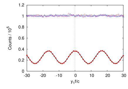
Figure 26: Computer simulation data of the single-particle and two-particle counts for the HBT experiment depicted in Fig. 25. Red open circles: EBCM results for the counts of detector $D_{0}$. Blue open triangles: EBCM results for the counts of detector $D_{1}$. Red closed circles: EBCM results for the coincidence counts. The dashed and solid lines are least-square fits of the predictions of wave theory to the EBCM data for the single detector and coincidence counts, respectively. Simulation parameters: $N_{\mathrm{tot}}=2\times 10^{5}$ events per $y_{1}f/c$-value, $N_{\mathrm{F}}=40$, $X=100000c/f$, $d=2000c/f$, $\gamma=\widehat{\gamma}=0.99$ and $N_{p}=2$.

VIII.2.2 EBCM simulation

In Fig. 26 we present the EBCM simulation results of the HBT experiment depicted in Fig. 25 with messengers that contain the time-of-flight and the angle $\xi$, see Eq. (26). For simplicity, we have put detector $D_{1}$ at $(X,0)$ and plot the single detectors and coincidence counts as a function of the $y$-position of detector $D_{0}$. In each simulation step, both sources $S_{0}$ and $S_{1}$ create a messenger with their initial time-of-flight set to some randomly chosen messages $\mathbf{y}_{n}$ ($n=0,1$) which are kept fixed for $N_{\mathrm{F}}$ successive pairs of messengers. Two pseudo-random numbers are used to determine whether the messengers travel to detector $D_{0}$ or $D_{1}$. The time-of-flights are given by

$$T_{n,m}=\frac{\sqrt{X^{2}+((1-2n)d/2-y_{m})^{2}}}{c},$$ (86)

where $n=0,1$ and $m=0,1$ label the source and detector, respectively. As Fig. 26 shows, averaging over the randomness in the initial messages wipes out all interference fringes in the single-detector counts, in agreement with Maxwell’s theory. Denoting the total number of emitted pairs of messengers by $N_{\mathrm{tot}}$, we find that the number of single-detector counts fluctuates around $N_{\mathrm{tot}}/2$, as expected from Maxwell’s theory, providing numerical evidence that the detectors have indeed 100% detection efficiency. Similarly, the data for the coincidence counts are in excellent agreement with the expression

$$N_{\mathbf{coincidence}}=\frac{N_{\mathrm{tot}}}{8}\left(1+\frac{1}{2}\cos 2\pi f\Delta T\right),$$ (87)

predicted by Maxwell’s theory.

For simplicity, we have confined the above presentation to the case of a definite polarization. Simulations with randomly varying polarization (results not shown) are also in concert with Maxwell’s theory. Elsewhere, we show that three-photon interference can be modeled by an EBCM as well Jin et al. (2010c).

VIII.2.3 Nonclassicality

From Eq. (87), it follows that the visibility of the interference fringes, defined by

$${\cal V}=\frac{\max(N_{\mathbf{coincidence}})-\min(N_{\mathbf{coincidence}})}{\max(N_{\mathbf{coincidence}})+\min(N_{\mathbf{coincidence}})},$$ (88)

cannot exceed 50%. It seems commonly accepted that the visibility of a two-photon interference experiment exceeding 50% is a criterion of the nonclassical nature of light. On the other hand, according to Ref. Agafonov et al. (2008), the existence of high-visibility interference in the third and higher orders in the intensity cannot be considered as a signature of three- or four-photon interference. Thus, it seems that the two-photon case may be somewhat special, although there is no solid argument why this should be so.

As in the case of the EPRB experiment, HBT experiments employ time-coincidence to measure the intensity-intensity correlations. It is therefore quite natural to expect that a model that purports to explain the observations accounts for the time delay that occurs between the time of arrival at a detector and the actual click of that detector. In quantum theory, time is not an observable and can therefore not be computed within the theory proper, hence there is no way that these time delays, which are being measured, can be accounted for by quantum theory. Consequently, any phenomenon that depends on these time delays must find an explanation outside the realm of quantum theory (as it is formulated to date).

It is straightforward to add a time-delay mechanism to the EBCM of the detector. As an illustrative example, we assume that the time of the detector click, relative to the time of emission, is given by

$$t_{\mathrm{delay}}=T_{n,m}+rT_{\mathrm{max}}(1-|\mathbf{T}|^{2})^{h},$$ (89)

where $0<r<1$ is a pseudo-random number, and $\mathbf{T}$ is given by Eq. (57). The time scale $T_{\mathrm{max}}$ and the exponent $h$ are free parameters of the time-delay model. Coincidences are counted by comparing the difference between the delay times of detectors $D_{0}$ and $D_{1}$ with a time window $W$, exactly in the same way as is done in the EPRB experiment (see Eq. (77).

From the simulation results presented in Fig. 27, it is clear that by taking into account that there are fluctuations in the time delay that depend on the time-of-flight and the internal state of the detector, the visibility changes from ${\cal V}=50\%$ to ${\cal V}\approx 100\%$. In Fig. 27, the solid line represents the least square fit of $a(1+b\cos 2\pi f\Delta t)$ to the simulation data.

This example demonstrates that a purely classical corpuscular model of a two-photon interference experiment can yield visibilities that are close to 100%, completing the picture that high visibilities in two-, three- or four-photon interference experiments can be explained within the realm of a classical theory, such as an EBCM. In any case, the commonly accepted criterion of the nonclassical nature of light needs to be be revised.

The time delay model Eq. (89) is perhaps one of the simplest that yield interesting results but it is by no means unique. The study of various time delay models with applications to fermion and boson statistics will be published elsewhere.

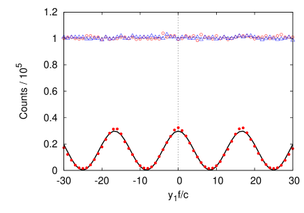
Figure 27: Computer simulation data of the single-particle and two-particle counts for the HBT experiment depicted in Fig. 25, generated by the same EBCM that produced the data of Fig. 26 extended with the time-delay model Eq. (89). Red open circles: EBCM results for the counts of detector $D_{0}$. Blue open triangles: EBCM results for the counts of detector $D_{1}$. Red closed circles: EBCM results for the coincidence counts. The dashed and solid lines are least-square fits of the predictions of wave theory to the EBCM data for the single detector and coincidence counts, respectively. Simulation parameters: $N_{\mathrm{tot}}=2\times 10^{5}$ events per $y_{1}f/c$-value, $N_{\mathrm{F}}=40$, $X=100000c/f$, $d=2000c/f$, $\gamma=\widehat{\gamma}=0.99$, $N_{p}=2$, $W=2/f$, $T_{\mathrm{max}}=2000/f$ and $h=8$.

IX Summary and outlook

We have demonstrated that one universal event-based corpuscular model (EBCM) for the interaction of photons with matter suffices to explain the interference and correlation phenomena that are observed when individual photons are detected one by one. Of course, this model produces the frequency distributions for observing many photons that are in full agreement with the predictions of Maxwell’s theory and quantum theory. This is not surprising: Maxwell’s theory is used as a guiding principle to determine the single-event dynamics of the model. The main conclusion of these simulations is that the effects such as EPR correlations and enhanced visibility in two-photon interference in the HBT experiment are contained in a corpuscular model of light and simply appear as the result of the particular processing of the detection events. The EBCM is entirely classical in the sense that it uses concepts of the macroscopic world and makes no reference to quantum theory but is nonclassical in the sense that it does not rely on the rules of classical Newtonian dynamics.

It is remarkable that the observations of all the fundamental quantum optics experiments covered in this paper can be explained using a computer simulation model that is elementary. All that is required is elementary algebra and some Euclidian geometry. This is in sharp contrast with the mathematical machinery that has to be mastered in order to understand the meaning of the symbols used to formulate Maxwell’s theory or quantum theory.

One may agrue that a finite-difference time-domain (FDTD) Maxwell solver Taflove and Hagness (2005) also carries out very simple arithmetic operations but the point is that the simple update rules for the electromagnetic-field variables are derived from a set of differential (or integral) equations. In contrast, in the EBCM approach, the rules are constructed such that the stationary state of the classical, dynamical system of processing units yields the intensity distribution of the wave problem, not the other way around. In other words, for quantum optics experiments, Maxwell’s theory and quantum theory arecontained in the EBCM presented in this paper. We consider it unlikely that this EBCM is unique: There may be several ways to modify the update rule of the processors such that the stationary state of the EBCM agrees with the prediction of Maxwell’s theory,

An important question is whether the event-based corpuscular model can make predictions that can be tested experimentally. From the nine examples presented in this work, it is clear that after a few hunderds of photons have been processed by the EBCM, the frequencies of observations are hardly distinghuisable from the intensities expected from Maxwell’s theory (recall that the EBCM of the detector has 100% detection efficiency) Therefore, to test the EBCM, one has to concieve an experiment that is capable of testing the transient regime of the EBCM, that is the regime before the EBCM reaches its stationary state,. Elsewhere we have proposed an experiment with a Mach-Zehnder interferometer that might be used for this purpose Richter et al. (2010). We hope that our simulation results will stimulate the design of new time-resolved single-photon experiments to test our corpuscular model for optical phenomena.

We would like to draw attention to the fact that the EBCM approach may have practical applications as a new method for simulating optical phenomena. From a computation viewpoint, the salient features of our event-based approach are:

• It yields the stationary solution of the Maxwell equations by simulating particle trajectories only.

• Material objects are represented by DLM-based units placed on a boundary of these objects, which in practice involves some form of discretization. Disregrading this discretization, all calculations are performed using Euclidean geometry.

• Artifacts due to the unavoidable termination of the simulation volume which are inherent to wave equation solvers Taflove and Hagness (2005) are absent: Particles that leave the simulation volume can simply be removed from the simulation.

• Unlike wave equation solvers which may consume substantial computational resources (i.e. memory and CPU time) to simulate the propagation of waves in free space, it calculates the motion of the corresponding particles in free space at almost no computational cost.

• Modularity: Starting from the unit that simulates the behavior of a plane interface between two homogeneous media other optical components can be constructed by repeated use of the same unit.

The work presented in this paper may open a route to rigorously include the effects of interference in ray-tracing software. For this purpose, it may be necessary to extend the DLM-based model for a lossless dielectric materials to, say a Lorentz model for the response of material to the electromagnetic field Taflove and Hagness (2005) and to extend the model to simulate phenomena that, in Maxwell’s theory, are due to evanescent waves. We leave these extensions for future research.

X Aknowledgement

We would like to thank K. De Raedt and S. Miyashita for many helpful comments. This work is partially supported by NCF, the Netherlands.

Deterministic Learning Machines

We begin by asking the following simple question: Given a real number $0\leq y\leq 1$ how can we generate a sequence of binary variables $y_{1},\ldots,y_{K}=0,1$ such that their average $(y_{1}+\ldots+y_{K})/K$ yields a good (in a certain sense to be defined later) approximation for $y$?

.1 Pseudo-random machine

Perhaps the most obvious answer to this question is the following: Use a pseudo-random number generator to produce numbers $0<r_{1},\ldots,r_{K}\leq 1$ and to set $y_{k}=0$ ($y_{k}=1$) if $r_{k}\leq y$ ($r_{k}>y$). If the pseudo-random number generator is any good, we expect that $(y_{1}+\ldots+y_{K})/K\approx y$ if $K$ is large but much less than the period of the pseudo-random number generator Press et al. (2003). Theoretically, we can analyze the properties of these sequences by imagining that there exist a device that generates random variables in the Kolmogorov sense. Then, we would have

$$\lim_{K\rightarrow\infty}\frac{1}{K}\sum_{k=1}^{K}y_{k}\stackrel{{\scriptstyle P}}{{\rightarrow}}y,$$ (90)

where the notation $A\stackrel{{\scriptstyle P}}{{\rightarrow}}B$ means that $A$ is equal to $B$ with probability one, which in plain words means it is likely that $A=B$ but that it can happen that $A\not=B$. For sufficiently large $K$, probability theory tells us that with $K$ binary variables, we can represent of the order of $1/c(d)\sqrt{K}$ real numbers, where $c(d)$ is proportional to the number of significant digits $d$ of these real numbers De Raedt et al. (2006b).

Thus, when we use (pseudo) random numbers, the problem can be solved in a rather trivial manner. But can we do better and dispose of random numbers altogether? Yes, we can and perhaps surprisingly, the algorithm De Raedt et al. (2005b) that follows is not more complicated than the simplest algorithms that are used to generate pseudo random numbers Press et al. (2003).

.2 Deterministic learning machine I

Let us consider a machine that receives as input messages in the form of numbers $0\leq y_{k}\leq 1$ for $k=1,2,\ldots$. For each $y_{k}$ that it receives, the machine updates its internal state, represented by $0\leq x_{k}\leq 1$ according to

$$x_{k}=\gamma x_{k-1}+(1-\gamma)\Delta_{k},$$ (91)

where $\Delta_{k}=\Theta(|\gamma x_{k-1}+(1-\gamma)-y_{k}|-|\gamma x_{k-1}-y_{k}|)$ with $\Theta(.)$ denoting the unit step function. In words, the machine will choose the new internal state $x_{k}$ such that the difference with the input $y_{k}$ is minimum De Raedt et al. (2005b). The sequence $\Delta_{1},\Delta_{2},\ldots$ are the output messages of the machine. The parameter $0\leq\gamma<1$ controls both the speed and accuracy with which the machine can learn the input value $y_{k}$ De Raedt et al. (2005b, 2006b). As a detailed mathematical analysis of the dynamics of the machine defined by the rule Eq. (91) is given in Ref. De Raedt et al., 2006b, it will not be repeated here.

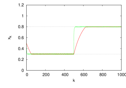
Figure 28: The internal state of the DLM as a function of the number of input events $k$. Red line: DLM defined by the update rule Eq. (91). Green line: DLM defined by the update rule Eq. (93).

Here, we illustrate the operation of the DLM defined by update rule Eq. (91) by a simple example in which we feed the DLM by a sequence of 500 messages with fixed value $y_{k}=0.3$ followed by another 500 messages with fixed value $y_{k}=0.8$. Initially the machine is in the state $x_{0}=1/2$ and $\gamma=0.99$.

In Fig. 28 (red line) we show simulation results of the internal state $x_{k}$ of the DLM as a function of the number of events $k$ that have been received by the DLM. From Eq. (91), $x_{0}=0.5$ and $y=0.3$ it immediately follows that initially $\Delta_{k}=0$ and that it takes about $k_{0}=(\log 0.3-\log 0.5)/\log 0.99\approx 51$ events for the internal vector to reach a state where $x_{k}\approx y_{k}=0.3$ (for $k\leq 500$), in concert with the data of Fig. 28 (red line).

Once the DLM has reached this regime, its behavior changes drastically: With $y_{k}$ still fixed, its internal vector will start oscillating about $y_{k}$. If $x_{k}$ decreases (increases), the machine generates $\Delta_{k}=0(1)$ as output De Raedt et al. (2005b, 2006b). It can be shown that in this stationary regime (and this regime only) with fixed input value $y_{k}=y$, the average $K^{-1}\sum_{k=1}^{K}\Delta_{k}=N/K$ is an optimal, rational approximation to $y$, optimal in the sense that the variance of the bit stream is minimal, implying that subsequences of the $\Delta_{k}$’s yield obviously less accurate but again optimal approximations De Raedt et al. (2005b, 2006b). In plain words, the sequence of $\Delta_{k}$’s is such that each subsequence yields an approximation to the fixed input $y_{k}=y$.

From Fig. 28 (red line), it is clear that if we change the input from $y_{k}=0.3$ for $k\leq 500$ to $y_{k}=0.8$ for $501\leq k\leq 1000$, the machine needs about eighty input events to reach the new stationary state This relaxation process would take even much longer if we would have chosen $\gamma=0.999$ instead of $\gamma=0.99$. Thus, for this very simple machine, there is a trade off between accuracy and the time it needs to respond to significant changes of the input value.

It is not difficult to modify the machine such that it responds much faster to changes of the input value. As one particular example of such a modification, consider the machine defined by the rules

$$\gamma^{\prime} = \min(1-|x_{k-1}-y_{k}|,\gamma),$$ (92)

$$x_{k} = \gamma^{\prime}x_{k-1}+(1-\gamma^{\prime})\Delta_{k}.$$ (93)

In Fig. 28 (green line), we present the results of a simulation in which we feed the DLM defined by Eqs. (92) and (93) by a sequence of 500 messages with fixed value $y_{k}=0.3$ followed by another 500 messages with fixed value $y_{k}=0.8$. Comparing the results of the DLMs defined by Eq. (91) and Eqs. (92),(93), respectively, it is clear that the former responds much slower to changes in the input than the latter.

It should be noted that there is nothing special about the DLM defined by Eq. (92): There are many ways to improve the response time by letting $\gamma^{\prime}$ depend on the input, the current state and $\gamma$, some examples being given later. It should be noted though that if DLMs are used to construct event-based processes that reproduce the results of wave mechanics, the only requirement is that these results are being reproduced in the regime where the DLMs have reached the stationary state, that is after many events have been processed.

.3 Deterministic learning machine II

The DLM of Section .1 encodes the data (a real number) contained in messages it receives in its internal state and for each message it receives, generates as output a one-bit message. If the input messages are constant over a sufficiently long period, the stream of output bits is an accurate representation of the input data. From the description of this machine, it is rather obvious that it can be generalized to accept messages that contain several real numbers.

In this section, we consider a different type of DLM, namely a DLM that updates its internal state such that it represents the average of the data contained in the input messages. Specifically, we consider messages containing as data $d$-dimensional unit vectors $\mathbf{v}_{k}$ (Euclidian norm $\|\mathbf{v}_{k}\|=1$) and a DLM with an internal state represented by a $d$-dimensional vector $\mathbf{x}_{k}$.

The state of the DLM is updated according to the rule

$$\mathbf{x}_{k}=\gamma\mathbf{x}_{k-1}+(1-\gamma)\mathbf{v}_{k},$$ (94)

where $0<\gamma<1$ and Euclidian norm of the initial internal state is assumed to satisfy $\|\mathbf{x}_{0}\|\leq 1$. The formal solution of Eq. (94) reads,

$$\mathbf{x}_{k}=\gamma^{k-k^{\prime}}\mathbf{x}_{k^{\prime}}+(1-\gamma)\sum_{j=k^{\prime}+1}^{k}\gamma^{k-j}\mathbf{v}_{j},$$ (95)

for all $0\leq k^{\prime}<k$. From Eq. (95) it immediately follows that $\|\mathbf{x}_{k}\|\leq\gamma^{k}\|\mathbf{x}_{0}\|+1-\gamma^{k}\leq 1$ for all $k\geq 1$, meaning that the vectors representing the internal state of the DLM can never leave the $d$-dimensional sphere of radius one. In other words, the update rule Eq. (95) defines a numerically stable iterative procedure.

Note the amount of internal storage that this DLM uses is “as large” as the storage needed to represent the data contained in a single message and that the last term Eq. (95) has the structure of a convolution of the input data $\mathbf{v}_{j}$ and a “memory” kernel $\gamma^{j}$.

From the formal solution Eq. (95), the fact that in practice the sequence $\{{\bf v}_{1},{\bf v}_{2},\cdots,{\bf v}_{K}\}$ is finite, and the usual trick to assume a periodic continuation of the sequence, we have

$${\bf x}_{mK} = \gamma^{K}{\bf x}_{(m-1)K}+(1-\gamma)\sum_{j=(m-1)K+1}^{mK}\gamma^{mK-j}{\bf v}_{j}$$ (96)

$$= \gamma^{K}{\bf x}_{(m-1)K}+(1-\gamma)\sum_{j=1}^{K}\gamma^{K-j}{\bf v}_{j+(m-1)K}$$

$$= \gamma^{K}{\bf x}_{(m-1)K}+(1-\gamma){\bf f}_{K},$$

where

$${\bf f}_{K}=\sum_{j=1}^{K}\gamma^{K-j}{\bf v}_{j},$$ (97)

and $m\geq 0$. From Eq. (96) we find

$${\bf x}_{mK}=\gamma^{mK}{\bf x}_{0}+(1-\gamma)\frac{1-\gamma^{mK}}{1-\gamma^{K}}{\bf f}_{K},$$ (98)

and hence

$$\lim_{m\rightarrow\infty}{\bf x}_{mK}=\frac{1-\gamma}{1-\gamma^{K}}\sum_{j=1}^{K}\gamma^{K-j}{\bf v}_{j},$$ (99)

such that

$$\lim_{\gamma\rightarrow 1^{-}}\lim_{m\rightarrow\infty}{\bf x}_{mK}=\frac{1}{K}\sum_{j=1}^{K}{\bf v}_{j}.$$ (100)

From Eq. (100), we conclude that as $\gamma\rightarrow 1^{-}$ the internal vector converges to the time average of the vectors $\mathbf{v}_{1},\mathbf{v}_{2},\cdots,\mathbf{v}_{K}$.

Some analytical insight into the behavior of this DLM can be obtained by assuming that $\mathbf{x}_{k}$ and $\mathbf{v}_{k}$ are the values of time-dependent vectors $\mathbf{x}(t)$ and $\mathbf{v}(t)$ sampled at regular time intervals $\tau$. If $\mathbf{x}(t)$ allows a Taylor series expansion, we may write $\mathbf{x}_{k}=\mathbf{x}(\tau k)$, $\mathbf{x}_{k-1}=\mathbf{x}(\tau k)-\tau d\mathbf{x}(t)/dt|_{t=\tau k}+{\cal O}(\tau^{2})$ such that the update rule Eq. (94) can be expressed as

$$\frac{d\mathbf{x}(t)}{dt}=-\frac{1-\gamma}{\tau\gamma}\mathbf{x}(t)+\frac{1-\gamma}{\tau\gamma}\mathbf{v}(t).$$ (101)

In order that Eq. (101) makes sense for $\tau\rightarrow 0$, we must have $\lim_{\tau\rightarrow 0}(1-\gamma)/\tau\gamma=\Gamma$. This requirement is trivially satified by putting $\gamma=1/(1+\tau\Gamma)$. Then Eq. (101) takes the form of the first-order linear differential equation

$$\frac{d\mathbf{x}(t)}{dt}=-\Gamma\mathbf{x}(t)+\Gamma\mathbf{v}(t).$$ (102)

The formal solution of Eq. (102) reads

$$\mathbf{x}(t)=e^{-t\Gamma}\mathbf{x}(0)+\Gamma\int_{0}^{t}e^{-u\Gamma}\mathbf{v}(t-u)du.$$ (103)

As in Eq. (95), the last term Eq. (103) has the structure of a convolution of the input data $\mathbf{v}(u)$ and the memory kernel $e^{-u\Gamma}$. From the derivation of Eq. (102), it follows that if we interpret $\tau$ as the time interval between two successive messages and let $\tau$ approach zero, then $\gamma=1/(1+\tau\Gamma)$ approaches one and the DLM defined by the update rule Eq. (94) “solves” the differential equation Eq. (102). Therefore, we may view Eq. (102) as a course-grained, continuum approximation to the discrete, event-by-event process defined by Eq. (94).

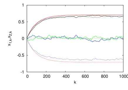
Figure 29: The two components of the internal vector ${\mathbf{x}}_{k}=(x_{1,k},x_{2,k})$ as a function of the number of received events $k$ for four different input messages ${\mathbf{e}}_{k}=(1,-1)/\sqrt{2}$ (red lines) with statistical average $(1,-1)/\sqrt{2}$, ${\mathbf{e}}_{k}=(r^{1/2}_{k},(1-r_{k})^{1/2})$ (black lines) with statistical average $(2/3,2/3)$, ${\mathbf{e}}_{k}=(\cos\pi r_{k},-\sin\pi r_{k})$ (blue lines) with statistical average $(0,2/3)$, and ${\mathbf{e}}_{k}=(\cos 2\pi r_{k},\sin 2\pi r_{k})$ (green lines) with statistical average $(0,0)$, $0\leq r_{k}<1$ being uniform pseudo-random numbers. Solid lines: $x_{1,k}$; Dashed lines: $x_{2,k}$. In all cases ${\mathbf{x}}_{0}=(0,0)$ and $\gamma=0.99$.

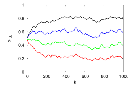
Figure 30: The first components of the internal vector ${\mathbf{x}}_{k}=(x_{1,k},x_{2,k})$ of a DLM that has two input ports to receive messages. A message arriving on input port 0(1) is represented by $\mathbf{v}_{k}=(1,0)$ ($\mathbf{v}_{k}=(0,1)$). The probability that a message arrives on input port 0(1) is $p_{0}$ ($1-p_{0}$). Initially, the DLM is in the state ${\mathbf{x}}_{0}=(1/2,1/2)$ and $\gamma=0.99$. Red line: $p_{0}=0.2$; Green line: $p_{0}=0.4$; Blue line: $p_{0}=0.6$; Black line: $p_{0}=0.8$. This DLM estimates the frequency with which the messages arrive on input ports 0 and 1.

As an illustration of how this DLM can be used, we consider two simple cases:

1. A DLM with one input port receiving messages represented by a two-dimensional unit vector $\mathbf{v}_{k}$. According to Eq. (100), after the DLM has received enough events such that it reached its stationary state, its internal state represents the time average of the events, that is we have ${\bf x}_{K}\approx K^{-1}\sum_{k=1}^{K}\mathbf{v}_{k}$ of $\gamma\lesssim 1$. In Fig. 29, we present some simulation results for different random vectors $\mathbf{v}_{k}$. In all cases, the internal state shows the expected behavior, namely it converges to the time-average of the input data. Note that the DLM has no information about the total number of events.

2. A DLM that receives messages (the precise content of which is of no importance here) on either input port “0” or input port “1” (but never on both ports simultaneously) and has its initial state set such that $x_{1,0}+x_{2,0}=1$. Then, setting $\mathbf{v}_{k}=(1,0)$ ($\mathbf{v}_{k}=(0,1)$) if the message arrives thought port 0 (1), it follows directly from Eq. (100) that $x_{1,k}+x_{2,k}=1$ for all $k\geq 1$ and that as a result, the internal state of the DLM will converge to the relative frequencies with which the messages arrive on ports 0 and 1. Some illustative simulation results are presented in Fig. 30, showing that this DLM can be employed to estimate from a time series of two different types of events, the relative frequency of these events.

For later applications, it is of the utmost importance that these DLMs can estimate averages without having to count the total number of events (which in real optics experiments is not known). From Figs. 28 and 29, it is clear that it may take quite a number of event for the DLMs to reach their stationary state. If necessary, the relaxation time can be reduced (significantly) by adding a rule that changes $\gamma$, analogous to the trick we introduced in Section .2 Jin et al. (2010a).

References

- Born and Wolf (1964) M. Born and E. Wolf, Principles of Optics (Pergamon, Oxford, 1964).
- Paul (2004) H. Paul, Introduction to Quantum Optics (Cambridge University Press, Cambridge, 2004).
- Garrison and Chiao (2009) J. C. Garrison and R. Y. Chiao, Quantum Optics (Oxford University Press, Oxford, 2009).
- Grangier et al. (1986) P. Grangier, G. Roger, and A. Aspect, Europhys. Lett. 1, 173 (1986).
- Kocher and Commins (1967) C. A. Kocher and E. D. Commins, Phys. Rev. Lett. 18, 575 (1967).
- Merli et al. (1976) P. G. Merli, G. F. Missiroli, and G. Pozzi, Am. J. Phys. 44, 306 (1976).
- Tonomura et al. (1989) A. Tonomura, J. Endo, T. Matsuda, T. Kawasaki, and H. Ezawa, Am. J. Phys. 57, 117 (1989).
- Tonomura (1998) A. Tonomura, The Quantum World Unveiled by Electron Waves (World Scientific, Singapore, 1998).
- Roychoudhuri (2010) C. Roychoudhuri, in Quantum Theory: Reconsideration of Foundations - 5, edited by A. Khrennikov (AIP Conference Proceedings, Melville and New York, 2010), vol. 1232, pp. 143 – 152.
- Mandel (1999) L. Mandel, Rev. Mod. Phys. 71, S274 (1999).
- von Neumann (1955) J. von Neumann, Mathematical Foundations of Quantum Mechanics (Princeton University Press, Princeton, 1955).
- Ballentine (2003) L. E. Ballentine, Quantum Mechanics: A Modern Development (World Scientific, Singapore, 2003).
- Home (1997) D. Home, Conceptual Foundations of Quantum Physics (Plenum Press, New York, 1997).
- De Raedt et al. (2005a) H. De Raedt, K. De Raedt, and K. Michielsen, Europhys. Lett. 69, 861 (2005a).
- De Raedt et al. (2005b) K. De Raedt, H. De Raedt, and K. Michielsen, Comp. Phys. Comm. 171, 19 (2005b).
- De Raedt et al. (2005c) H. De Raedt, K. De Raedt, and K. Michielsen, J. Phys. Soc. Jpn. Suppl. 76, 16 (2005c).
- Michielsen et al. (2005) K. Michielsen, K. De Raedt, and H. De Raedt, J. Comput. Theor. Nanosci. 2, 227 (2005).
- De Raedt et al. (2006a) K. De Raedt, K. Keimpema, H. De Raedt, K. Michielsen, and S. Miyashita, Euro. Phys. J. B 53, 139 (2006a).
- De Raedt et al. (2007a) H. De Raedt, K. De Raedt, K. Michielsen, K. Keimpema, and S. Miyashita, J. Phys. Soc. Jpn. 76, 104005 (2007a).
- De Raedt et al. (2007b) K. De Raedt, H. De Raedt, and K. Michielsen, Comp. Phys. Comm. 176, 642 (2007b).
- De Raedt et al. (2007c) H. De Raedt, K. De Raedt, K. Michielsen, K. Keimpema, and S. Miyashita, J. Comp. Theor. Nanosci. 4, 957 (2007c).
- Zhao and De Raedt (2008) S. Zhao and H. De Raedt, J. Comp. Theor. Nanosci. 5, 490 (2008).
- Zhao et al. (2008a) S. Zhao, H. De Raedt, and K. Michielsen, Found. of Phys. 38, 322 (2008a).
- Zhao et al. (2008b) S. Zhao, S. Yuan, H. De Raedt, and K. Michielsen, Europhys. Lett. 82, 40004 (2008b).
- Jin et al. (2010a) F. Jin, S. Yuan, H. De Raedt, K. Michielsen, and S. Miyashita, submitted to J. Phys. Soc. Jpn. (2010a).
- Jin et al. (2010b) F. Jin, S. Zhao, S. Yuan, H. De Raedt, and K. Michielsen, J. Comp. Theor. Nanosci. (in press) (2010b), http://arxiv.org/abs/0908.1036.
- Jin et al. (2010c) F. Jin, H. De Raedt, and K. Michielsen, Commun. Comput. Phys. 7, 813 (2010c).
- Jacques et al. (2007) V. Jacques, E. Wu, F. Grosshans, F. Treussart, P. Grangier, A. Aspect, and J.-F. Roch, Science 315, 966 (2007).
- Schwindt et al. (1999) P. D. D. Schwindt, P. G. Kwiat, and B.-G. Englert, Phys. Rev. A 60, 4285 (1999).
- Mizobuchi and Ohtaké (1992) Y. Mizobuchi and Y. Ohtaké, Phys. Lett. A 186, 1 (1992).
- Unnikrishnan and Murthy (1996) C. Unnikrishnan and S. Murthy, Phys. Lett. A 221, 1 (1996).
- Brida et al. (2004) G. Brida, M. Genovese, M. Gramegna, and E. Predazzi, Phys. Lett. A 328, 313 (2004).
- Aspect et al. (1982a) A. Aspect, P. Grangier, and G. Roger, Phys. Rev. Lett. 49, 91 (1982a).
- Aspect et al. (1982b) A. Aspect, J. Dalibard, and G. Roger, Phys. Rev. Lett. 49, 1804 (1982b).
- Weihs et al. (1998) G. Weihs, T. Jennewein, C. Simon, H. Weinfurther, and A. Zeilinger, Phys. Rev. Lett. 81, 5039 (1998).
- Hadfield (2009) R. H. Hadfield, Nature Photonics 3, 696 (2009).
- de Broglie (1925) L. de Broglie, Annales de Physique 3, 22 (1925).
- Jönsson (1961) C. Jönsson, Zeitschrift für Physik 161, 454 (1961).
- Noel and Stroud Jr (1995) M. W. Noel and C. R. Stroud Jr, Phys. Rev. Lett. 75, 1252 (1995).
- Zeilinger et al. (1988) A. Zeilinger, R. Gähler, C. G. Shull, W. Treimer, and W. Mampe, Rev. Mod. Phys. 60, 1067 (1988).
- Rauch and Werner (2000) H. Rauch and S. A. Werner, Neutron Interferometry: Lessons in Experimental Quantum Mechanics (Oxford Univ. Press, London, 2000).
- Carnal and Mlynek (1991) O. Carnal and J. Mlynek, Phys. Rev. Lett. 66, 2689 (1991).
- Keith et al. (1991) D. W. Keith, C. R. Ekstrom, Q. A. Turchette, and D. E. Pritchard, Phys. Rev. Lett. 66, 2693 (1991).
- Arndt et al. (1999) M. Arndt, O. Nairz, J. Vos-Andreae, C. Keller, G. van der Zouw, and A. Zeilinger, Nature 401, 680 (1999).
- Brezger et al. (2002) B. Brezger, L. Hackermüller, S. Uttenthaler, J. Petschinka, M. Arndt, and A. Zeilinger, Phys. Rev. Lett. 88, 100404 (2002).
- Jacques et al. (2005) V. Jacques, E. Wu, T. Toury, F. Treussart, A. Aspect, P. Grangier, and J.-F. Roch, Eur. Phys. J. D 35, 561 (2005).
- Feynman et al. (1965) R. P. Feynman, R. B. Leighton, and M. Sands, The Feynman Lectures on Physics, Vol. 3 (Addison-Wesley, Reading MA, 1965).
- Pfleegor and Mandel (1967) R. Pfleegor and L. Mandel, Phys. Rev. 159, 1084 (1967).
- DS (0) http://demonstrations.wolfram.com/EventByEventSi mulationOfDoubleSlitExperimentsWithSinglePhoto/.
- Trieu et al. (2010) B. Trieu, K. Michielsen, and H. De Raedt, submitted to Comp. Phys. Comm. (2010).
- (51) J. A. Wheeler, in: Mathematical foundations of quantum theory, Proc. New Orleans Conf. on The mathematical foundations of quantum theory, ed. A.R. Marlow (Academic, New York, 1978) [reprinted in Quantum theory and measurements, eds. J.A. Wheeler and W.H. Zurek (Princeton Univ. Press, Princeton, NJ, 1983) pp. 182-213].
- Jacques et al. (2008) V. Jacques, E. Wu, F. Grosshans, F. Treussart, P. Grangier, A. Aspect, and J.-F. Roch, Phys. Rev. Lett. 100, 220402 (2008).
- Scully and Drühl (1982) M. O. Scully and K. Drühl, Phys. Rev. A 25, 2208 (1982).
- Kim et al. (2000) Y. H. Kim, R. Yu, S. P. Kulik, Y. Shih, and M. O. Scully, Phys. Rev. Lett. 84, 1 (2000).
- Aharonov and Zubairy (2005) Y. Aharonov and M. S. Zubairy, Science 307, 875 (2005).
- Scully et al. (1991) M. O. Scully, B.-G. Englert, and H. Walther, Nature 351, 111 (1991).
- Kwiat et al. (1992) P. G. Kwiat, A. M. Steinberg, and R. Y. Chiao, Phys. Rev. A 45, 7729 (1992).
- Pittman et al. (1996) T. B. Pittman, D. V. Strekalov, A. Migdall, M. H. Rubin, A. V. Sergienko, and Y. H. Shih, Phys. Rev. Lett. 77, 1916 (1996).
- Walborn et al. (2002) S. P. Walborn, M. O. T. Cunha, S. Pádua1, and C. H. Monken, Phys. Rev. A 65, 033818 (2002).
- Scarcelli et al. (2007) G. Scarcelli, Y. Zhou, and Y. Shih, Eur. Phys. J. D 44, 167 (2007).
- Ghose et al. (1991) P. Ghose, D. Home, and G. Agarwal, Phys. Lett. A 153, 403 (1991).
- Bose (1897) J. Bose, Proc. R. Soc. 62, 300 (1897).
- De Raedt et al. (2007d) H. De Raedt, K. Michielsen, S. Miyashita, and K. Keimpema, Euro. Phys. J. B 58, 55 (2007d).
- Grimmet and Stirzaker (1995) G. R. Grimmet and D. R. Stirzaker, Probability and Random Processes (Clarendon Press, Oxford, 1995).
- Pascazio (1986) S. Pascazio, Phys. Lett. A 118, 47 (1986).
- Bell (1993) J. S. Bell, Speakable and unspeakable in quantum mechanics (Cambridge University Press, Cambridge, 1993).
- de la Peña et al. (1972) L. de la Peña, A. Cetto, and T. Brody, Lett. Nuovo Cim. 5, 177 (1972).
- Fine (1974) A. Fine, Synthese 29, 257 (1974).
- Fine (1982a) A. Fine, Synthese 50, 279 (1982a).
- Fine (1982b) A. Fine, Phys. Rev. Lett. 48, 291 (1982b).
- Fine (1982c) A. Fine, J. Math. Phys. 23, 1306 (1982c).
- de Muynck (1986) W. M. de Muynck, Phys. Lett. A 114, 65 (1986).
- Jaynes (1989) E. T. Jaynes, in Maximum Entropy and Bayesian Methods, edited by J. Skilling (Kluwer Academic Publishers, Dordrecht, 1989), vol. 36, p. 1.
- Brody (1993) T. Brody, The Philosphy Behind Physics (Springer, Berlin, 1993).
- Fine (1996) A. Fine, The Shaky Game: Einstein Realism and the Quantum Theory (University of Chicago Press, Chicago, 1996).
- Khrennikov (1999) A. Y. Khrennikov, Interpretations of Probability (VSP Int. Sc. Publishers, Utrecht, 1999).
- Sica (1999) L. Sica, Opt. Comm. 170, 55 (1999).
- De Baere et al. (1999) W. De Baere, A. Mann, and M. Revzen, Found. Phys. 29, 67 (1999).
- Hess and Philipp (2001) K. Hess and W. Philipp, Proc. Natl. Acad. Sci. USA 98, 14228 (2001).
- Hess and Philipp (2005) K. Hess and W. Philipp, in Foundations of Probability and Physics-3, edited by A. Khrennikov (AIP Conference Proceedings, Melville, New York, 2005), vol. 750, p. 150.
- Accardi (2005) L. Accardi, in Foundations of Probability and Physics-3, edited by A. Khrennikov (AIP Conference Proceedings, Melville, New York, 2005), vol. 750, p. 21.
- Kracklauer (2005) A. F. Kracklauer, in Foundations of Probability and Physics-3, edited by A. Khrennikov (AIP Conference Proceedings, Melville, New York, 2005), vol. 750, p. 219.
- Santos (2005) E. Santos, Phil. Mod. Phys. 36, 544 (2005).
- Morgan (2006) P. Morgan, J. Phys. A 39, 7441 (2006).
- Khrennikov (2007) A. Y. Khrennikov, in Foundations of Probability and Physics-4, edited by G. Adenier, C. A. Fuchs, and A. Y. Khrennikov (AIP Conference Proceedings, Melville, New York, 2007), vol. 889, p. 7.
- Adenier and Khrennikov (2007) G. Adenier and A. Y. Khrennikov, J. Phys. B: At. Mol. Opt. Phys. 40, 131 (2007).
- Nieuwenhuizen (2009) T. M. Nieuwenhuizen, in Foundations of Probability and Physics - 5, edited by L. Accardi, G. Adenier, C. Fuchs, G. Jaeger, A. Khrennikov, J. A. Larsson, and S. Stenholm (AIP Conference Proceedings, Melville and New York, 2009), vol. 1101, p. 127.
- Matzkin (2009) A. Matzkin, in Foundations of Probability and Physics - 5, edited by L. Accardi, G. Adenier, C. Fuchs, G. Jaeger, A. Khrennikov, J. A. Larsson, and S. Stenholm (AIP Conference Proceedings, Melville and New York, 2009), vol. 1101, p. 339.
- (89) H. De Raedt, K. Hess, and K. Michielsen, Extended Boole-Bell inequalities applicable to quantum theory, http://arxiv.org/abs/0901.2546.
- Brown and Twiss (1956) R. H. Brown and R. Q. Twiss, Nature 178, 1046 (1956).
- Glauber (1963a) R. J. Glauber, Phys. Rev. Lett. 10, 84 (1963a).
- Glauber (1963b) R. J. Glauber, Phys. Rev. 130, 2529 (1963b).
- Agafonov et al. (2008) I. N. Agafonov, M. V. Chekhova, T. S. Iskhakov, and A. N. Penin, Phys. Rev. A 77, 053801 (2008).
- Taflove and Hagness (2005) A. Taflove and S. Hagness, Computational Electrodynamics: The Finite-Difference Time-Domain Method (Artech House, Boston, 2005).
- Richter et al. (2010) M. Richter, K. Michielsen, T. Lippert, B. Barbara, S. Miyashita, and H. De Raedt, submitted to Europhys. Lett. (2010).
- Press et al. (2003) W. H. Press, B. P. Flannery, S. A. Teukolsky, and W. T. Vetterling, Numerical Recipes (Cambridge University Press, Cambridge, 2003).
- De Raedt et al. (2006b) H. De Raedt, K. De Raedt, K. Michielsen, and S. Miyashita, Comp. Phys. Comm. 174, 803 (2006b).