Kelvin-Helmholtz instabilities in Smoothed Particle Hydrodynamics

Abstract

In this paper we investigate whether Smoothed Particle Hydrodynamics (SPH), equipped with artificial conductivity, is able to capture the physics of density/energy discontinuities in the case of the so-called shearing layers test, a test for examining Kelvin-Helmholtz (KH) instabilities. We can trace back each failure of SPH to show KH rolls to two causes: i) shock waves travelling in the simulation box and ii) particle clumping, or more generally, particle noise. The probable cause of shock waves is the Local Mixing Instability (LMI), previously identified in the literature. Particle noise on the other hand is a problem because it introduces a large error in the SPH momentum equation.

The shocks are hard to avoid in SPH simulations with initial density gradients because the most straightforward way of removing them, i.e. relaxing the initial conditions, is not viable. Indeed, by the time sufficient relaxing has taken place the density and energy gradients have become prohibitively wide. The particle disorder introduced by the relaxation is also a problem. We show that setting up initial conditions with a suitably smoothed density gradient dramatically improves results: shock waves are reduced whilst retaining relatively sharp gradients and avoiding unnecessary particle disorder. Particle clumping is easy to overcome, the most straightforward method being the use of a suitable smoothing kernel with non-zero first central derivative. We present results to that effect using a new smoothing kernel: the LInear Quartic (LIQ) kernel.

We also investigate the role of artificial conductivity (AC). Although AC is necessary in the simulations to avoid “oily” features in the gas due to artificial surface tension, we fail to find any relation between using artificial conductivity and the appearance of seeded KH rolls. Including AC is necessary for the long-term behavior of the simulation (e.g. to get $\lambda=1/2,1$ KH rolls). In sensitive hydrodynamical simulations great care is however needed in selecting the AC signal velocity, with the default formulation leading to too much energy diffusion. We present new signal velocities that lead to less diffusion.

The effects of the shock waves and of particle disorder become less important as the time-scale of the physical problem (for the shearing layers problem: lower density contrast and higher Mach numbers) decreases. At the resolution of current galaxy formation simulations mixing is probably not important. However, mixing could become crucial for next-generation simulations.

1 Introduction

Smoothed Particle Hydrodynamics (SPH) is a lagrangian technique to solve the equations of hydrodynamics. It was first conceived by Lucy (1977) and Gingold & Monaghan (1977) to solve astrophysical problems. Because the differential equations are solved on a particle mesh that moves with the flow, adaptivity to accomodate large density variations is inherent to SPH. As shown in Tasker et al. (2008) SPH indeed has the advantage over grid-based techniques when it comes to problems with a large dynamic range. However, when it comes to handling steep density gradients SPH codes have to acknowledge their superiors in grid-based codes.

Recently, doubt has been cast upon whether SPH is able to capture all of the physics related to discontinuities. Agertz et al. (2007) highlighted a known problem in SPH: the formation of an artificial gap around density discontinuities. Previous allusions to this problem are found in e.g. Cummins & Rudman (1999), where a method to enforce incompressibility in SPH is proposed. Tartakovsky & Meakin (2005) propose a method to overcome this problem: use the local number density instead of the normal density to weigh SPH variables. This shifts the problem from requiring a continuous density to a continuous number density. The latter can be achieved by setting up the initial conditions such that the low density fluid uses SPH particles with lower mass, instead of less SPH particles with the same mass. Agertz et al. (2007) furthermore argue that a basic SPH scheme is unable to exhibit Kelvin-Helmholtz or Rayleigh-Taylor instabilities when a density gradient is involved. In a follow-up paper, Read et al. (2010) identify two main problems with standard SPH implementations: the Local Mixing Instability (LMI) and the “E0” error in the momentum equation. The LMI is the cause of the artificial gap problem highlighted above, whereas the problem with the E0 error in the SPH momentum equation has previously been highlighted by Morris (1996). Read et al. (2010) present a solution to these problems based on a temperature-weighted density and a modified smoothing kernel.

Price (2008) presents a different solution to the artificial gap problem. Based on the general approach previously outlined by Monaghan (1997) he introduces an “artificial conductivity” (AC) term into the equations. This term induces a certain amount of energy diffusion across energy discontinuities, allowing a discontinuity (which SPH is unable to handle properly) to become more “smeared out” and thus treatable with SPH.

Kawata et al. (2009) present their implementation of an SPH scheme, closely tailored after the scheme by Rosswog & Price (2007), which includes the artificial conductivity term. They present the basic tests performed by Agertz et al. (2007): the blob test and the shearing layers test. Their results indicate that the Price (2008) AC solution gives improved performance for the blob test, on the condition that enough particles are present in the blob. Their shearing layers test (with a density contrast of 9.6) exhibits Kelvin-Helmoltz instabilities for a Kelvin-Helmholtz time-scale of $\tau_{\mathrm{KH}}=0.57$.

Interestingly, Okamoto et al. (2003) investigated shearing flows in SPH. They find that noisiness in the SPH smoothing of variables gives rise to small-scale pressure gradients which significantly decelerate the shearing flow.

In § 2 we give a brief introduction to the SPH code, highlighting the implementation of artificial conductivity (AC). A new smoothing kernel with non-zero central first derivative is presented in § 3. Various aspects of the shearing layers test are then examined in § 4 and a discussion is given in § 5.

Most of the plots in this paper were made using HYPLOT. HYPLOT is a freely available open source analysis package, with an emphasis on SPH. Currently only GADGETII file reads are supported. HYPLOT uses PyQt4 for its GUI frontend, matplotlib for the plotting and a host of C++ classes for the actual computations. Interested users are recommended to get the latest snapshot from the svn repository.

2 The Code

We use the publicly available version of the Nbody/SPH code GADGETII (Springel, 2005). There are two base premises when formulating a Smoothed Particle Hydrodynamics (SPH) solution to the equations of hydrodynamics:

1. the integral representation of field functions,

2. the particle approximation.

In the first premise a function is replaced by its integral representation, given by the integration of the multiplication of that function and a smoothing kernel function. The second premise states that the integral from the first premise is replaced by a discretized summation using a set of particles in the support domain. The latter is a key approximation as it obsoletes the use of a background mesh for numerical integration. Both premises allow us to use the following simple equation to calculate the density at a certain point in space $\mn@boldsymbol{r}$:

$$\rho(\mn@boldsymbol{r})=\sum_{i=1}^{N}m_{j}W(|\mn@boldsymbol{r}-\mn@boldsymbol{r}_{i}|,h),$$ (1)

where the summation goes over all the particles within the support domain, delimited by the smoothing length $h$. Here, $m_{j}$ is the mass of the $j$th particle, $W$ is a smoothing function.

For a derivation of the SPH formulation of the basic equations of hydrodynamics we refer the reader to e.g. Springel & Hernquist (2002), where the equations are derived from a Lagrangian variational principle.

2.1 Artificial Conductivity

From e.g. Monaghan (1997) and Price (2008) we learn that an artificial conductivity (AC) term should be included in the SPH equations when dealing with energy discontinuities. The expression for the dissipational part (i.e. without the adiabatic part) of the energy equation for an SPH particle $i$ then becomes:

$$\left(\frac{\mathrm{d}u_{i}}{\mathrm{d}t}\right)_{\mathrm{diss}}= \sum_{j}\frac{m_{j}}{\bar{\rho}_{ij}}\Big{[}-\frac{1}{2}\alpha v_{\mathrm{sig}}(\mn@boldsymbol{v}_{ij}\cdot\hat{\mn@boldsymbol{e}}_{ij})^{2}$$

$$\qquad+\alpha_{u}v_{\mathrm{sig}}^{u}(u_{i}-u_{j})\Big{]}\hat{\mn@boldsymbol{e}}_{ij}\cdot\overline{\mn@boldsymbol{\nabla}_{i}W_{ij}},$$ (2)

with $u$ the specific energy. The summation over $j$ is the sum over all neighbours of particle $i$. Here, $m_{j}$ is the neighbour particle mass, $\bar{\rho}_{ij}=(\rho_{i}+\rho_{j})/2$ with $\rho_{i}$ the standard SPH particle density. $\alpha$ and $\alpha_{u}$ are coefficients that can be used to dynamically vary the contribution of the terms based on the presence of e.g. local velocity convergence. We set $\alpha=\alpha_{u}=1$ and $v_{\mathrm{sig}}=(c_{i}+c_{j}-\beta\mn@boldsymbol{v}_{ij}\cdot\hat{\mn@boldsymbol{e}}_{ij})$, with $c_{i}$ the sound speed of particle $i$. Note that the first term in equation (2) with $\beta$ set to $1.5$ is equal to the artificial viscosity (AV) employed in the GADGETII code (Springel, 2005), apart from the Balsara switch. The second term in eq. (2) is the artificial conductivity (AC) term.

Price (2008) suggests the following form for the AC signal velocity $v_{\mathrm{sig}}^{u}$:

$$v_{\mathrm{sig}}^{u}=\sqrt{\frac{|P_{i}-P_{j}|}{\bar{\rho}_{ij}}},$$ (3)

with $P_{i}$ and $P_{j}$ the pressures of respectively particles $i$ and $j$. With this choice, spurious pressure gradients across contact discontinuities are gradually eliminated. We note however that as the expression for the artificial conductivity (2) is actually an SPH representation of a diffusion term (Price, 2008), using the suggested signal velocity (eq. (3)) could lead to spurious energy diffusion. When using this signal velocity to eliminate pressure discontinuities one implicitly assumes that lower energy corresponds with lower pressure, as the sign of the energy transfer is determined by the energy gradient whilst the magnitude of the transfer is determined by both the energy and pressure gradients. If this assumption is valid the diffusion will distribute energy from the high-energy particles to the low-energy particles, reducing the pressure discontinuities. In the simulations we use the equation of state for an ideal gas:

$$p=(\gamma-1)\rho u,$$ (4)

with $p$ the pressure, $\gamma$ the adiabatic constant (typically taken to be 5/3, the value for an ideal mono-atomic gas). From eq. (4) we learn that we can only know that higher energy corresponds to higher pressure when the density is constant. If the low-energy particles have higher pressure, the situation will not reach the desired pressure equilibrium as energy will flow from the high-energy particles to the low-energy particles, increasing the pressure discontinuities. In this case energy will keep flowing until an approximate energy equilibrium is reached. It is straightforward to formulate a signal velocity that does not suffer from this problem:

$$v_{\mathrm{sig,1}}^{u}=\mathrm{sign}\left[(P_{i}-P_{j})(u_{i}-u_{j})\right]\sqrt{\frac{|P_{i}-P_{j}|}{\bar{\rho}_{ij}}},$$ (5)

where the sign of the energy diffusion is now determined by the sign of the pressure gradient. Expanding on this idea, another possible form of the signal velocity is:

$$v_{\mathrm{sig,2}}^{u}=\mathrm{sign}\left[(\tilde{P}_{i}-\tilde{P}_{j})(u_{i}-u_{j})\right]\sqrt{\frac{|\tilde{P}_{i}-\tilde{P}_{j}|}{\bar{\rho}_{ij}}},$$ (6)

where $\tilde{P}$ is the SPH-averaged pressure:

$$\tilde{P}_{i}=\sum_{i=1}^{N}m_{\mathrm{j}}A_{j}\rho^{\gamma-1}_{j}\bar{W}(|\mn@boldsymbol{r}-\mn@boldsymbol{r}_{i}|,h),$$ (7)

with $A_{j}$ the entropy of particle $j$, $\bar{W}=(W_{i}+W_{j})/2$. The advantage of this form is that the artificial conductivity counteracts pressure differences at the fluid level, not at the particle level. A disadvantage is the extra overhead needed to compute and store $\tilde{P}$. Note that (as highlighted by Price (2008)) the formulations for the signal velocity shown here (eqs. (3), (5) and (6)) are not applicable when gravity is involved, because typically under hydrostatic equilibrium a configuration with constant pressure is not an equilibrium configuration. A signal velocity applicable in an environment with gravity, e.g. a modified version of eq. (3), can also be extended with the factor we added here in going from eq. (3) to eq. (5).

It is worth considering whether the potential errors induced by equation (3) actually happen, and if so if their magnitude is of an order that requires fixing. To test this we set up two simulations, one using the signal speed of eq. (3), the other using eq. (5). These simulations consist of two central smoothed density gradients and constant pressure, exactly the same way we set up simulations for the shearing layers tests (section 4). Initial specific energies are set on a per-particle basis using the calculated SPH density and a fixed constant pressure value. To be able to clearly examine the influence of the conductivity the SPH particles are fixed in place. Results are shown in Fig. 1.

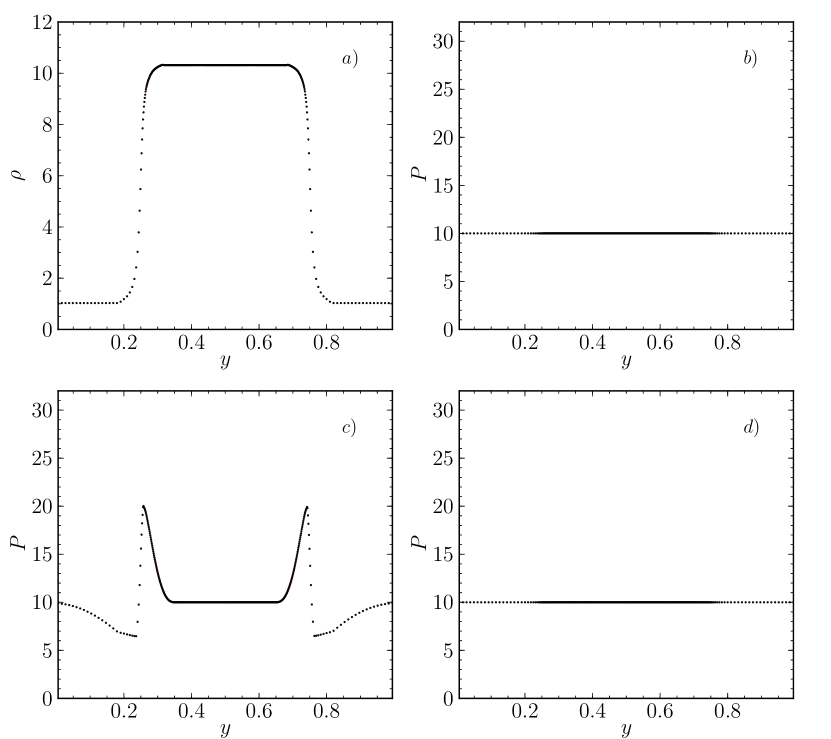
Figure 1: a) Initial density along the $y$-axis for an $x$-slice [0,0.001]. b) Initial pressure along the $y$-axis. c) Pressure along the $y$-axis at time $t=2$ in the case of the standard AC signal velocity (eq. (3)). d) Pressure along the $y$-axis at time $t=2$ in the case of the modified AC signal velocity (eq. (5)).

We immediately see that the simulation with the signal velocity as in eq. (3) (panel $c$) indeed exhibits divergent behavior. SPH particles with low energy ($0.25<x<0.75$) receive extra energy, increasing their pressure, and vice versa for particles with high energy. Once this mechanism is set in motion it is self-amplifying. The simulation with the modified signal velocity on the other hand (panel $d$) does not exhibit any special behavior, the pressure remains constant, as expected. Note that the reason the divergent behavior is set in motion in this setup is numerical noise. Indeed, from eq. (3) one would expect a simulation with equal particle pressures to have a signal velocity which is equal to zero everywhere. As we set the initial particle specific energies based on the required constant pressure value ($P=10$) and the calculated density, we can expect that calculating back to the pressure later on (again using eq. (4)) will yield non-zero albeit very small pressure differences. This does not imply that the unwanted energy diffusion is a result of numerical artifacts, because in a real simulation there will always be non-zero pressure differences and we can expect at any time to have too much energy diffusion. On the other hand, because in a real simulation the SPH particles are not fixed in place they will react to the increased pressure gradient, trying to erase it. The buildup of diffusion will thus not be as drastical as the one shown in Fig. 1. We will investigate the new forms of the AC signal velocities further on.

3 LIQ Kernel

A vital part of any SPH code is the smoothing kernel $W$. The attention given to the smoothing kernel is however somewhat limited, with people generally using the cubic spline kernel (see e.g. Kawata et al., 2009). Schuessler & Schmitt (1981) already demonstrated that the choice of the smoothing kernel can have a large impact on simulations. More recently, Morris (1996); Price (2005); Read et al. (2010) performed a linear perturbation analysis of the SPH equations of motion for different kernels, examining the stability of these kernels for longitudinal (related to the clumping instability) and transversal waves. They show several smoothing kernels with a zero central derivative that suffer from the clumping instability (also dubbed tensile instability).

Various approaches have been suggested to deal with this. One possiblity is to modify the SPH equations. Monaghan (2000) advocates including an artificial pressure term. Sigalotti et al. (2009) on the other hand apply an adaptive kernel density estimation algorithm (ADKE). A different approach is to take a different form for the smoothing kernel. The advantage of the latter approach is that no modifications to the actual SPH scheme are necessary. The disadvantage is that bell-shaped kernels (with central derivative equal to zero) tend to give better results for a wide range of test cases as compared to hyperbolic or parabolic shaped kernels (Fulk, 1996).

Here we construct a new smoothing kernel with non-zero central derivative: the LInear Quartic or LIQ kernel. We note several earlier approaches: the HYDRA kernel by Thomas & Couchman (1992), who artificially modified the cubic spline (CS) kernel to have a constant central first derivative (by fixing it to $-1/\pi$ for $x\leq 2/3$). This approach was recently picked up by Merlin et al. (2009). Johnson et al. (1996) employed a quadratic kernel, resulting in a linear first derivative. More recently Read et al. (2010) modified the central part of the cubic spline kernel with their Core-Triangle (CT) kernel, giving it a non-zero central first derivative. We will come back to these at the end of section 3.1.

We assume a kernel of the form:

$$W(\mn@boldsymbol{r},h)=\frac{W_{\mathrm{r}}(u)}{h^{d}},$$ (8)

with $u=r/h$ and $d$ the number of dimensions. For $W_{\mathrm{r}}$ we take the following functional form:

$$W_{\mathrm{r}}=N\times\begin{cases}f_{1}:F-u&0\leq u<x_{\mathrm{s}}\\ f_{2}:Au^{4}+Bu^{3}+Cu^{2}+Du+E&x_{\mathrm{s}}\leq u<1\\ 0&1\leq u\end{cases}.$$ (9)

$x_{\mathrm{s}}$ is a free parameter determining the connection point of the polynomial and linear functions. This form is inspired by two ideas: (i) we want the smoothing kernel to be smooth (ii) the first derivative of the smoothing kernel should be a monotonously ascending function (i.e. it can have constant parts, but it can never descend).

The equations for the smoothing kernel (9) have 7 free parameters: $A$ through $F$ and the normalization factor $N$. We fix them by imposing the following boundary conditions:

$$f_{2}(x_{\mathrm{s}}) = f_{1}(x_{\mathrm{s}})$$ (10a)

$$\frac{{\partial}{f_{2}}}{\partial{u}}(x_{\mathrm{s}}) = \frac{{\partial}{f_{1}}}{\partial{u}}(x_{\mathrm{s}})$$ (10b)

$$\frac{{\partial}^{2}{f_{2}}}{\partial{u}^{2}}(x_{\mathrm{s}}) = 0$$ (10c)

$$f_{2}(1) = 0$$ (10d)

$$\frac{{\partial}{f_{2}}}{\partial{u}}(1) = 0$$ (10e)

$$\frac{{\partial}^{2}{f_{2}}}{\partial{u}^{2}}(1) = 0$$ (10f)

$$\int_{V}W(\mn@boldsymbol{r},h)\ \mathrm{d\mn@boldsymbol{r}} = 1,$$ (10g)

which ensure a smooth (up to second order) transition between $f_{1}$ and $f_{2}$ at $x_{\mathrm{s}}$ and sufficiently smooth behavior for $f_{2}\rightarrow 0$ as $u\rightarrow 1$.

Three different kernels are shown in Fig. 2 in the twodimensional case. The LIQ kernel has a lower central value than the CT kernel, and a higher value outwards. Read et al. (2010) find that they need a large number of neighbors for the CT kernel to reduce the $E_{0}$ error of the momentum equation and to reduce the pressure blips at the boundaries. The $E_{0}$ error on particle $i$ is given by (Read et al., 2010):

$$\mn@boldsymbol{E}_{0,i}=\sum_{j}\frac{m_{j}}{\rho_{j}}\left(\frac{\rho_{i}}{\rho_{j}}+\frac{\rho_{j}}{\rho_{i}}\right)\overline{h\mn@boldsymbol{\nabla}W}$$ (11)

Fig. 3 shows a plot of particle $E_{0}$ errors as a function of $y$, for the CS, CT and LIQ kernels. The number of neighbors is kept equal (32), the setup is that of the RHO2 simulation (see Table 4 and Section 4). The difference between the CT and LIQ kernels on the one hand and the CS kernel on the other hand is big, with particle clumping giving rise to large $E_{0}$ errors, evidenced by the large scatter between the peaks. The results for the CT and LIQ kernels are comparable, with the LIQ kernel slightly in front, as can be seen from the reduced scatter away from the peak areas and the smaller maximum values overall. It would be interesting to perform the 3D simulations as performed by (Read et al., 2010) with the LIQ kernel, in this paper we restrict ourselves to 2D however. Both the LIQ and CT kernels have the desired properties for their respective first derivatives. Table 1 lists computed LIQ kernel coefficients for a range of $x_{\mathrm{s}}$ values. Analytical expressions for the coefficients can be found in appendix A.

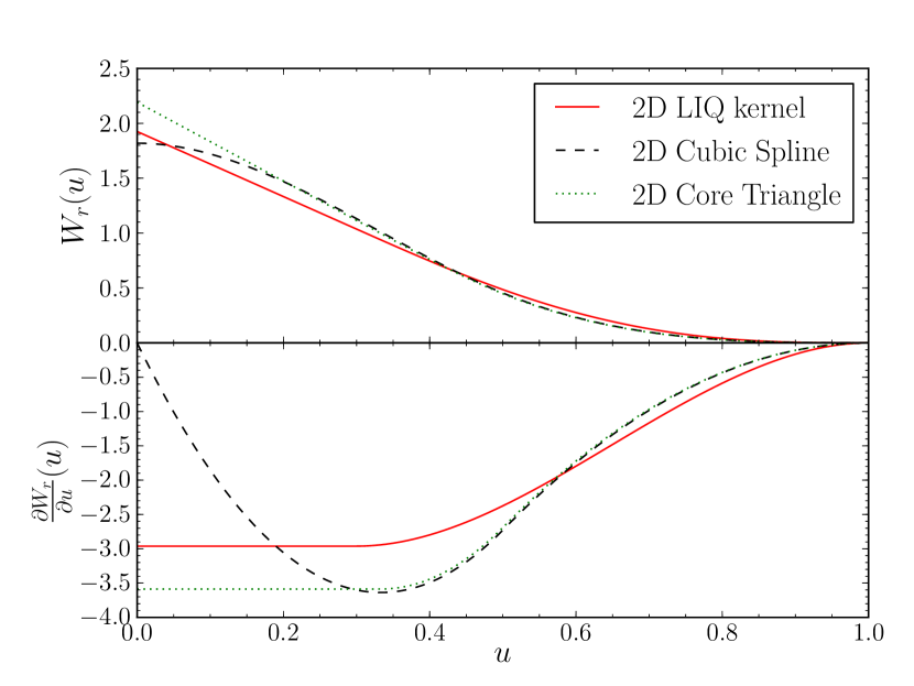
Figure 2: Upper panel. The 2D LIQ, CS and CT smoothing kernels. Lower panel. First derivative of these kernels.

Figure 3: The $E_{0}$ error for three shearing layers simulations ($t=0.5$) with, from top to bottom: the cubic spline kernel, the core triangle kernel, the linear quartic kernel. To guide the eye a binned mean value is also shown. The cyan line, shown in all panels, shows the values for the CS kernel. The green lines in panels $b$ and $c$ show the values for the respective CT and LIQ kernels.

Table 1: Coefficients of the LIQ Kernel (eq. (9)). The last two columns ($N_{\mathrm{2D}}$, $N_{\mathrm{3D}}$) give the norm $N$ respectively for two and three dimensions. See appendix A for analytical expressions.

$x_{\mathrm{s}}$	$A$	$B$	$C$	$D$	$E$	$F$	$N_{\mathrm{2D}}$	$N_{\mathrm{3D}}$
0	-0.5	1	0	-1	05	0.5	4.775	6.685
0.2	-0.9766	2.344	-1.172	-0.7813	0.5859	0.6	3.490	4.753
0.3	-1.458	3.790	-2.624	-0.2915	0.5831	0.6500	2.962	3.947
0.4	-2.315	6.481	-5.556	0.9259	0.4630	0.7	2.508	3.251
0.6	-7.813	25	-28.125	12.5	-1.563	0.8	1.798	2.168
0.8	-62.5	225	-300	175	-37.5	0.9	1.300	1.434

3.1 Fixing $x_{\mathrm{s}}$

To fix the remaining free parameter in the LIQ Kernel, the connection point $x_{\mathrm{s}}$, we set up a series of 2D Sod shock tube tests (Sod (1978), for recent use in SPH see e.g. Price (2008) (1D)). The $x$-range is $[0-0.1]$, the $y$-range $[0-1.5]$. The adiabatic index $\gamma$ is set to $5/3$. Further parameters can be found in table 2. Throughout this paper the number of SPH neighbours is 32, unless noted otherwise. Note that this number is actually quite high, with about 5–6 neighbours per dimension. The particles are set up on rows in the $y$-direction i.e. the initial $x$-separation between particles is equal everywhere. Results are shown in figure 4. From these results we learn that varying $x_{\mathrm{s}}$ has a major impact on the simulation. A value of 0.3 is optimal, with higher values resulting in a more noisy density profile and smaller values leading to small density oscillations in certain parts of the profile. The shock tube result with the LIQ kernel and $x_{\mathrm{s}}=0.3$ is slightly less good than that for the CS kernel (bottom right panel). The density found by the SPH summation using the LIQ kernel is less accurate than the density found using the CS kernel. The simulations in figure 4 started from the same initial conditions file, but have, depending on the value of $x_{\mathrm{s}}$, slightly different starting densities: the density is overestimated, the more so for smaller values of $x_{\mathrm{s}}$. Instead of lowering the particle masses to get identical initial density profiles we use identical masses in all simulations. The analytical shock-tube results shown in Fig. 4 are computed using the actual initial SPH densities.

Table 2: Sod shock tube test parameters. (1) density (2) specific energy (3) pressure (4) number of particles per $y$-column (5) total number of particles

	$\rho$	$u$	$P$	$N_{\mathrm{col}}$	$N$
high-density	1	1.5	1	400	20000
low density	0.25	1	0.1667	100	5000

In Fig. 5 we show the particle distribution on top of the rendered density, for a small region of the shock tube, at $t=0.2$. Overplotted is the circle of interaction for the same SPH particle. The clumping behavior in the left plot, using the CS kernel, is striking: particles form groups of 2. This behavior has been known for some time (see e.g. Schuessler & Schmitt, 1981). When using the LIQ kernel (right panel) there is no clumping. We note that this clumping does not lead to an actual decrease in resolution, as the circle of interaction for the SPH particle has a comparable radius in the two plots. Indeed, the clumping does not affect the actual size of the smoothing region. It does affect the homogeneity of the particles in that region, and through that it affects the validity of using an SPH estimate of a continuous integral (see section 2). As the CS kernel has been used extensively in SPH codes and found to give excellent results (see e.g. Springel, 2005; Price, 2008; Kawata et al., 2009, the shock tube results in Fig. 4), the SPH estimate of the integral does not seem to suffer from the clumping.

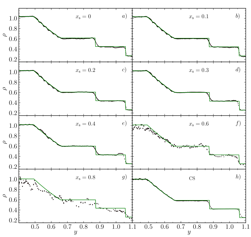
Figure 4: Results for the 2D Sod shock tube test with the LIQ Kernel, using varying connection points ($x_{\mathrm{s}}$). Only particles in the $x$-interval [0,0.005] are shown ($x$-range: [0,0.1]). Connection point values are shown in the plots. Panel $h)$ shows the result using the standard Cubic Spline kernel. The overplotted solid green line in each plot is the analytical solution.

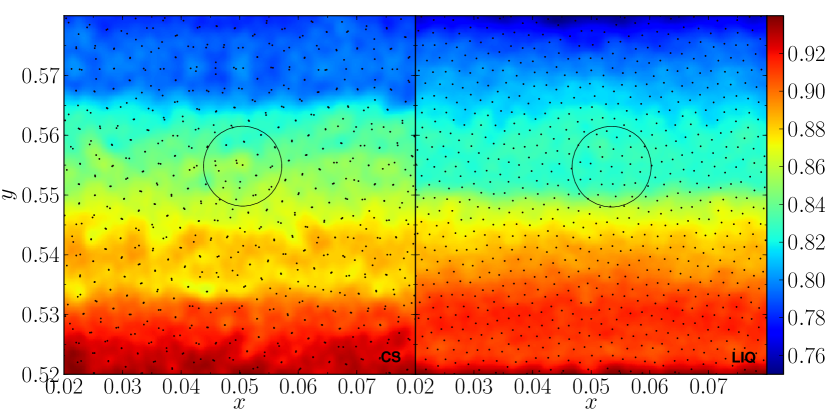
Figure 5: Particle distribution on top of the rendered density for a region in the shock tube test. Left panel: Cubic Spline. Right panel: LIQ Kernel. The overplotted circle is the region of influence for the same particle in both runs. The particle clumping in the left panel, using the CS kernel, is striking. No clumping is seen in the right panel.

In Fig. 6 we show the energy conservation of SPH for the 2D Sod shock-tube test for the HYDRA, Core Triangle, Johnson, LIQ ($x_{\mathrm{s}}=0.3$) and Cubic Spline kernels. As expected, the Cubic Spline kernel clearly leads to the best energy conservation. The behavior of the CT and LIQ kernels is similar, especially in their initial evolution. The Johnson and HYDRA kernels show the largest growth in their respective relative energy errors. Note that the HYDRA kernel is identical to the CS kernel, apart from the modified central first derivative. The resulting kernel does prevent clumping but the energy conservation leaves much to be desired. Moreover, among the family of LIQ kernels, the choice $x_{\mathrm{s}}=0.3$ turned out to provide the best energy conservation. The different result for the LIQ and CT kernels arises between $t=0.07$ and $t=0.15$. This interval corresponds to the time where the initial rectangular symmetry in the simulation breaks up. The initial energy error ($t<0.07$) thus shows the performance of the SPH scheme on a regular particle distribution whilst the late energy error ($t>0.15$) shows the performance with SPH particles having arranged themselves according to the respective smoothing kernels. The poor performance of the HYDRA kernel can be attributed to the artificial modification of the central derivative of the kernel, which breaks the conservative form of SPH. Note that all simulations use individual time-steps which in itself breaks the time-symmetry (and hence the energy conservation) of the integrator.

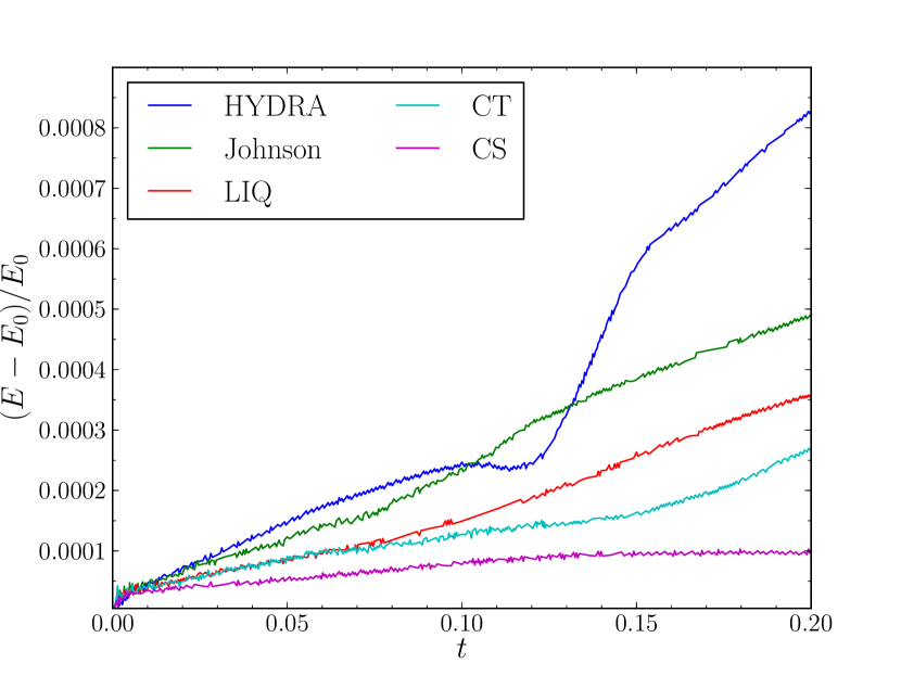
Figure 6: Relative energy error as a function of time, for a number of 2D shock-tube tests, using different smoothing kernels. Lines indicate, from top to bottom: HYDRA kernel (CS with modified central derivative), Johnson kernel (quadratic), LIQ kernel (see section 3, linear + 4${}^{\text{th}}$ order), CT kernel (centrally modified CS), Cubic Spline kernel (3${}^{\text{rd}}$ order). Note how modifying the central value of the derivative of the CS kernel drastically reduces energy conservation.

4 Shearing Layers Test

The shearing layers test, as presented by Agertz et al. (2007), is an excellent way of examining the ability of a hydrodynamical code to capture the formation of Kelvin-Helmholtz instabilities. These instabilities occur when two fluids have a relative velocity perpendicular to their contact layer. For an incompressible fluid there is an analytical expression for the time-scale for the growth of these Kelvin-Helmholtz instabilities (Chandrasekhar, 1961; Price, 2008):

$$\tau_{\mathrm{KH}}=\frac{2\pi}{\omega},$$ (12)

where

$$\omega=\frac{2\pi}{\lambda}\frac{(\rho_{1}\rho_{2})^{\frac{1}{2}}|v_{x,1}-v_{x,2}|}{(\rho_{1}+\rho_{2})}.$$ (13)

The indices 1 and 2 denote the two fluid layers. $\lambda$ is the wavelength of the perturbation. When re-written in terms of the density contrast $\chi$ ($\rho_{1}=\chi\rho_{2}$, we make the convention $\chi\geq 1$ e.g. the index 1 denotes the high-density layer):

$$\omega=\frac{2\pi}{\lambda}\frac{(\chi)^{\frac{1}{2}}|v_{x,1}-v_{x,2}|}{(1+\chi)}.$$ (14)

Various approaches have been suggested to enforce incompressibility in SPH (e.g. Cummins & Rudman, 1999; Hu & Adams, 2009). We use the weakly compressible SPH formulation, approximating incompressibility by using a small Mach number. Note that incompressibility is a requirement only for equation (14) to be valid, it is not a requirement for the simulations themselves to be valid.

KH instabilities are seeded by introducing an initial $y$-velocity perturbation following the prescription:

$$v_{y}=A\sin(2\pi x/\lambda).$$ (15)

All simulations, unless noted otherwise, have the following setup: the $x$- and $y$ ranges are 1. For the adiabatic index $\gamma$ we use a value of 5/3, as applicable for an ideal monoatomic gas. The density contrast $\chi$ is 10, with low- and high-density layers having a density of respectively 1 and 10. The respective specific energies are 15 and 1.5, resulting in respective sound speeds of 4.08 and 1.29. $\lambda$ is fixed at $1/6$, which should result in the initial growth of 6 KH density rolls. $A$ is set to 0.025. Note that we focus on a density contrast of 10, not 2, because preliminary tests showed us that an SPH code has much less trouble reproducing Kelvin-Helmholtz instabilities for lower density contrast: we concentrate on the more demanding test here. Previous studies of the KH instabilities either restrict themselves to a density contrast of 2 (Read et al., 2010; Merlin et al., 2009) or show KH tests with KH time-scales of 0.6 or lower (Price, 2008; Kawata et al., 2009).

4.1 Grid Code

To get a reference to compare the SPH results with we have conducted a series of Eulerian hydrodynamical simulations, using the FLASH code (version 3.2, (Fryxell et al. (2000); Dubey et al. (2008), see also http://flash.uchicago.edu)) . FLASH is an adaptive mesh refinement hydrodynamics code. Its standard hydro-solver uses the piecewise-parabolic method.

The KH simulation is run on a periodic 2D grid of size $1\times 1$. In order to avoid confusion from numerical issues as much as possible, we switched off the steepening algorithm for contact discontinuities and use just one refinement level, resulting in an effective resolution of $256^{2}$ = 65536 grid cells. We note that differences to runs with 2 refinement levels and contact steepening appear only after a few KH timescales, but are evident in the late stages of the higher Mach number runs presented here. The initial conditions are set as in the SPH simulations, without taking special care to smooth gradients, but keeping the idealised sharp discontinuity in density and velocity. Results are shown in Figs. 6 and 7 for two simulations with respective Mach numbers of 0.2 and 0.6. Those KH rolls that appear do so at times consistent with their respective $\tau_{\mathrm{KH}}$.

Results are shown in Figs. 7 and 8 for two simulations with respective Mach numbers of 0.2 and 0.6. Those KH rolls that appear do so at times consistent with their respective $\tau_{\mathrm{KH}}$ .

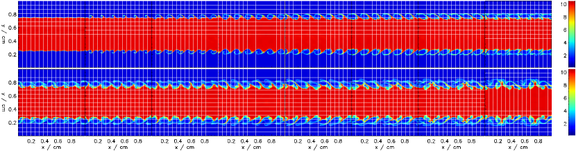
Figure 7: Grid simulation of the shearing layers test with $M=0.2$. Top row, left to right: $t=0.25,0.5,0.75,1,1.25,1.5,1.75,2$. Bottom row, left to right $t=2.25,2.5,2.75,3,3.25,3.5,3.75,4$: White boxes mark blocks of $16^{2}$ grid cells.

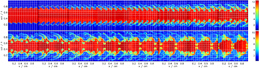
Figure 8: Grid simulation of the shearing layers test with $M=0.6$. Top row, left to right: $t=0.25,0.5,0.75,1,1.25,1.5,1.75,2$. Bottom row, left to right $t=2.25,2.5,2.75,3,3.25,3.5,3.75,4$: White boxes mark blocks of $16^{2}$ grid cells.

4.2 Standard SPH

We first examine the capability of standard SPH to handle the shearing layers problem. With standard SPH we mean SPH as implemented by e.g. Springel (2005) (which uses the entropy formulation of SPH) augmented with the artificial conductivity formalism (see section 2). This form of the SPH equations is rapidly becoming the standard (see e.g. Price, 2008; Kawata et al., 2009; Vanaverbeke et al., 2009; Merlin et al., 2009). We do this test for a range of Mach numbers, and thus for a range of Kelvin-Helmholtz time-scales (eq. (12)). The specific energies of the SPH particles were set after the density is computed, in order to force perfect pressure equilibrium (thus applying a crude smoothing of the IC). Details for the different simulations are listed in tables 3 and 4. Rendered plots of the density are shown in Fig. 10, for each run at its respective $\tau_{\mathrm{KH}}$ (see table 4). From Fig. 10 we learn that changing the Mach number in the simulation has a drastic impact on the formation of KH rolls: for small $M$ they are completely absent. The simulations of Price (2008) with $\chi=10$ have $M=0.775$ for the high-density layer, they are to be compared with SPH4. We thus find that the results in Price (2008), where artificial conductivity was enough to enable SPH to produce KH rolls, are only valid for high enough Mach numbers. In following sections we will try to improve on this situation. The situation at $t=2$ is shown in Fig. 11. It tells us that there is a large difference in the long-term evolution of the shearing layer simulations depending on the setup and the ingredients of the code. On the panels for $M=0.6$ (c, h and m) we should see $\lambda=1/2$ instabilities when comparing with the grid simulations in Fig. 8. Panel h shows a hint of these instabilities but they are very poorly developed. Panel m does better, the KH rolls appear although only on one side of the high-density layer.

Table 3: Velocities and $\tau_{\mathrm{KH}}$ for the different KH simulations. Rows from top to bottom: suffix: simulation number suffix (e.g. for the SPH series: SPH1-SPH5), $M$: Mach number of the high-density layer, $|v_{x}|$: absolute value of the $x$-velocity, $\tau_{\mathrm{KH}}$: KH time-scale (eq. (12))

suffix	1	2	3	4	5
$M$	0.2	0.4	0.6	0.8	1
$|v_{x}|$	0.26	0.52	0.77	1.0	1.3
$\tau_{\mathrm{KH}}$	1.23	0.56	0.37	0.28	0.22

Table 4: Parameters for the different KH simulations. series: Name for the simulation series, e.g. SPH1–SPH5. # part: Number of particles used. AC: Artificial conductivity included? (yes: X). kernel: Smoothing kernel used. $\rho$–smoothing: Type of density smoothing applied, if any.

series	SPH	RHO	LIQ	GRID	NOAC
# part	199252	184100	184100	200788	184100
AC	X	X	X	X	-
kernel	CS	CS	LIQ	CS/LIQ	LIQ
$\rho$–smoothing	-	column	column	grid	column

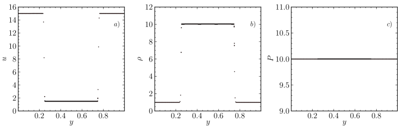
Figure 9: Initial specific energy (a), density (b) and pressure (c) as a function of $y$ for the SPH1-5 (see table 3) simulations. Only particles in the $x$-interval [0,0.005] are shown. Note that the specific energy of the particles at the contact discontinuity is smoothed in order to avoid a pressure blip.

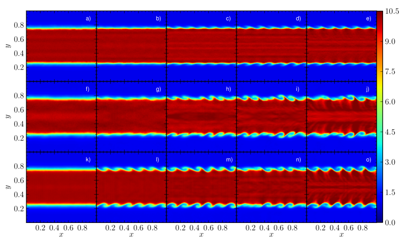
Figure 10: Density plots for shearing layers simulations (table 4) at their respective $\tau_{\mathrm{KH}}$ (table 3). Top row (a-e): from left to right: simulations SPH1-SPH5: standard SPH simulations. Middle row (f-j): RHO1-RHO5: standard SPH with a smoothed density setup. Bottom row (k-o): LIQ1-5: SPH with a smoothed density and using the LIQ kernel.

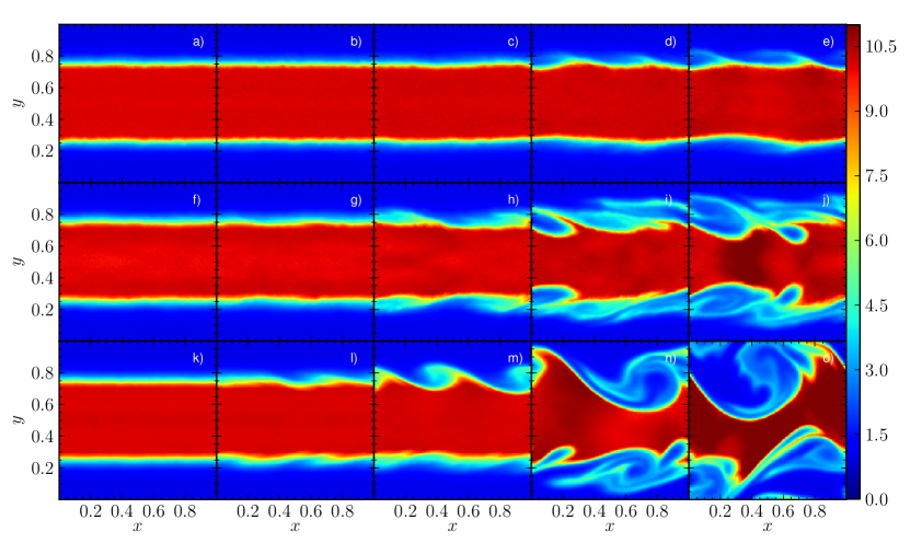
Figure 11: Same figure as Fig. 10, all figures now at $t=2$.

4.3 Standard SPH - Column-smoothed IC

We can expect the way the initial conditions for the shearing layers test were set up in the previous section to cause problems (as briefly mentioned by Hess & Springel (2009), though they do not try to formulate a remedy). SPH is inherently smoothed, and, in the current formulation, this particle smoothing is isotropic as the smoothing length is a scalar, not a vector nor a tensor. When one uses this formulation of SPH to tackle a problem where sharp discontinuities are present, as is the case in the shearing layers test, one is forcing SPH into a situation where its behavior is not well defined. Smoothing the initial particle energy based on the calculated initial density and a requested constant pressure value does not remedy this problem: it enforces equal pressures on a particle basis, which does not necessarily result in pressure equilibrium on a simulation basis. This is easy to see when making an analogy with the density: giving all particles an equal mass results in a constant density only if the particle distribution is homogeneous. Robertson et al. (2010) show that Eulerian codes exhibit similar problems, with numerical diffusion wiping out small-scale structures in the presence of a large bulk flow and sharp discontinuities. They present a different version of the KH test which does not suffer from this. We however do not discard the canonical test because the code is not able to solve it. We choose to modify the test so that we retain the physics of the original test whilst allowing the code to deal with it

Artificial conductivity goes a long way in preventing discontinuities as sharp as these from arising in simulations, but by the time AC has sufficiently smoothed the initial discontinuity a series of shocks has been created in the simulation volume. These are shown in Fig. 12. Depending on the time-scale of the growth of the instabilities these shocks will play a role in destroying emerging KH instabilities: the longer it takes for the instabilities to manifest themselves, the more they are wiped out by the travelling shock waves. When the shocks pass through the emerging instabilities a mixed layer is formed at the contact discontinuity. This layer acts as a lubricant, separating the two layers and thus preventing KH instabilities from developing. Only in the case where the KH instabilities form fast enough compared to the scale on which they are destroyed are they able to survive. This can be translated into a general paradigm: the longer it takes for KH rolls to manifest themselves in SPH, the more time there has been for SPH-induced deviations from the analytical, theoretical problem to destroy them. This explains why it is more easy to produce KH rolls for high Mach numbers. The origin of these shocks is probably related to the LMI, in the same way as the artificial gap problem. Imagine two particles with equal pressures, but different densities. If these particles approach each-other their respective densities will change towards equality. As entropy is conserved this implies, with $p=A\rho^{\gamma}$ (Springel & Hernquist, 2002), that these particles now have different pressures. As this process happens everywhere along the initial contact discontinuity this can set a shock-wave in motion. A possible cure for this problem is to smooth the regions where these discontinuities occur, giving rise to a net smaller LMI effect. To create a smooth interface we choose a function of the form:

$$\rho(y)=A\ \mathrm{atan}(B(y+C))+D,$$ (16)

where

$$A = \frac{\rho_{1}-\rho_{0}}{2\ \mathrm{atan}(\beta)}$$ (17)

$$B = 2\frac{\beta}{\delta}$$ (18)

$$C = -\frac{\delta}{2}$$ (19)

$$D = \frac{\rho_{1}+\rho_{2}}{2}$$ (20)

were fixed requiring (16) to be symmetrical around the boundary, scaling the argument of the $\mathrm{atan}$ such that $y=0,\delta$ resulted in an argument of respectively $-\beta,\beta$. For $\beta$ a value of 10 gives reasonable results, because $\mathrm{atan}(10)$ is close to $\pi/2$ (which is needed because it is connected to two constant-density functions). $\delta$ is the width of the boundary, which we took to be $(y_{\mathrm{max}}-y_{\mathrm{min}})/7.5$ for a part of the simulation box containing a single boundary layer e.g. $\delta=0.5/7.5$ in the current setup.

There are several methods to set up a smooth density. One method is to set up the particles in the two regions on two different grids. Within such a grid the $x$- and $y$ separations ($\Delta x$ and $\Delta y$ respectively) of particles are equal. Denoting one layer with the subscript 1, the other with 2, we have of course $\Delta x_{1}\neq\Delta x_{2}$ and $\Delta y_{1}\neq\Delta y_{2}$ when the layer densities differ. The smooth boundary between those grids can then be constructed by putting a number of equal-$y$ rows between those grids. The distance between these rows varies from $\Delta y_{1}$ to $\Delta y_{2}$ according to the square (in the 2D case) of some chosen function (e.g. eq. (16)). The number of particles on a row is then fixed by comparing the computed SPH density of particles on that row to the value of required analytical density $\rho_{\mathrm{an}}$ at that point. To get a perfect representation of the bounding function one would have to use an iterative scheme, varying the number of particles on the rows, recomputing the smoothing lengths and densities and repeating until convergence is reached. In our setup our prime concern is that the density is smooth, it is of little importance if the analytical boundary function is perfectly reproduced. We thus use a shortcut in generating the initial conditions: the SPH density on the $i$-th row $\rho_{i}$ is esimated by:

$$\rho_{i}=\frac{m_{i}}{\Delta x_{i}\Delta y_{i}},$$ (21)

with $m_{i}$ the particle mass on that row, $\Delta y_{i}$ the distance to the previous row and $\Delta x_{i}$ the interparticle distance. $\Delta x_{i}$, and from that the number of particles, can then be found from:

$$\Delta x_{i}=\frac{m_{i}}{\rho_{\mathrm{an}}\Delta y_{i}}.$$ (22)

Another method to construct a smooth density is to put all the SPH particles on columns (lines with constant $x$), with an equal and unchanged intercolumn distance. The smoothed density can then be attained by varying the interparticle separation within those columns. Finding those separations, using equation 21, is then a simple matter of using some bisection algorithm.

Simulations RHO1-5 correspond to the SPH1-5 series, with their initial density discontinuity smoothed using the first smoothed density method: particles on columns. Results are shown in Fig. 10. When comparing the top and middle rows we see that for $M\geq 0.6$ KH rolls have appeared. For $M=0.4$ some bumps are present, but these do not evolve into KH rolls. Although we have already greatly improved the situation, for low Mach numbers we are still unable to get adequate results. In Fig. 12 we can see that the magnitude of the shocks has decreased because of the density smoothing.

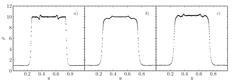
Figure 12: panel a. simulation SPH1 at $t=0.1$ (particles limited to $x$-interval [0,0.005]). One clearly sees shocks travelling inward from the contact discontinuities. panel b. simulation RHO1. Shocks are still present, although reduced in magnitude. panel c. density smoothing + the LIQ kernel.

4.4 Modified kernel - Column-smoothed IC

As mentioned in section 3 we can expect to do better in very sensitive simulations when using a smoothing kernel that does not cause particle clumping. In Fig. 10 we show results for the same simulations as the RHO1-RHO5 simulations (e.g. with smoothed density), but now using the LIQ kernel (see section 3). We see KH instabilities appear for $M\geq 0.4$, which is an improvement over the previous results where clear KH rolls appeared for $M\geq 0.6$. We also see that in general the shape of the KH rolls is much more symmetrical.

In figure 13 we show the pressure of the particles at roughly half the KH time-scale. When we look at the column smoothing results it is clear that the dominant shock in the RHO2 simulation, around $y=0.5$, is greatly reduced in magnitude in the LIQ2 simulation. This difference is mainly due to the different way the kernels respond to the initial conditions (particles initially on columns): the CS kernel is clearly not a good choice in this case. This is also demonstrated in the bottom right panel of Fig. 13, where a result for the CS kernel using grid smoothing is shown. It compares favourably with both LIQ2 results.

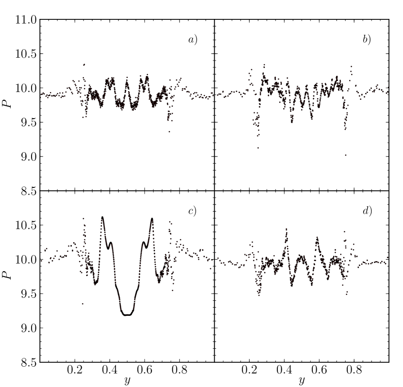
Figure 13: Pressure of SPH particles in the $x$-interval [0,0.005] as a function of $y$, at $t=0.25$, with $M=0.4$. The top row shows two runs with LIQ2 setup. The bottom row shows RHO2. The left panels have column density smoothing, the right panels have grid-based density smoothing.

4.4.1 Particle number

We can try increasing the particle number for the simulations with low Mach number, to see how it affects the KH rolls: simulations LIQ+1 and LIQ+2, each with $551\,100$ particles. Results are shown in Fig. 14. The LIQ+2 simulation, where KH rolls were already present in its low-resolution counterpart LIQ2, is seen to benefit a lot from the increased resolution: the KH rolls are much better defined. The situation for LIQ+1 however has not changed: KH rolls are still abscent at that resolution.

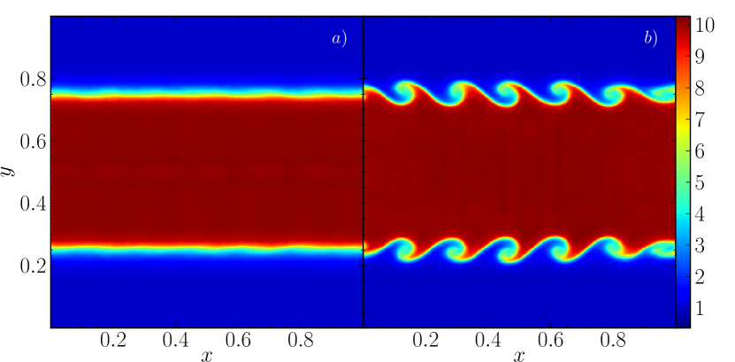
Figure 14: Density of two increased resolution shearing layers simulations at their respective $\tau_{\mathrm{KH}}$. panel a. LIQ+1 ($M=0.2,551\,100$ particles). panel b. LIQ+2 ($M=0.4,551\,100$ particles).

4.5 Grid-based density smoothing

We have also constructed initial conditions using the second smooth interface method: the two different layers consist of two different grids, with two smooth interfaces at the contacts. The energies of the particles are set using the same algorithm as before: after the SPH densities are computed the particle specific energies are set based on a constant pressure value. Part of the initial particle distribution is shown in Fig. 15. The simulation shown uses the LIQ kernel. Results for $M=0.2$ are shown in Fig. 16. On the density plot we see that no KH rolls manifest themselves: the same shocks that were present in the LIQ1 simulation are present here. We thus find that the artificial conductivity is not able to smooth away initial energy discontinuities fast enough to prevent the LMI from triggering these shock-waves. In the right panel we show the rendered density of the RHO2 simulation, using grid-based density smoothing (see also Fig. 13). The observed ripples at the contact discontinuities are a slight improvement over the RHO2 simulation shown in figure 10. The particle clumping does however prevent the KH rolls from growing to the same size as their LIQ2 counterparts.

In figure 17 we show the destruction of the KH instabilities by a shock wave in detail. From bottom to top we can see the wave passing through the emerging KH instabilities, erasing them.

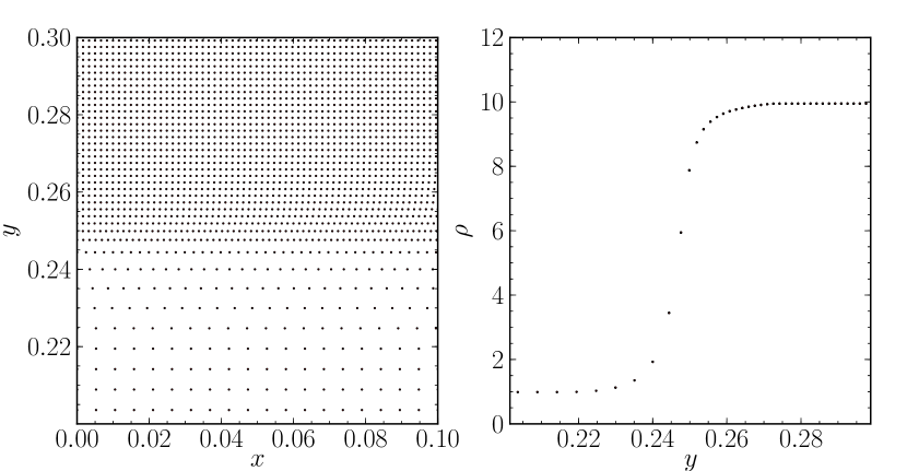
Figure 15: Initial conditions with smooth boundary from section 4.5 Left panel: At the top and bottom we can see the high- and low density grids respectively. A smoothly varying layer lies in between. Right panel: SPH-computed density as a function of $y$, for the particles in the left panel. The density varies smoothly.

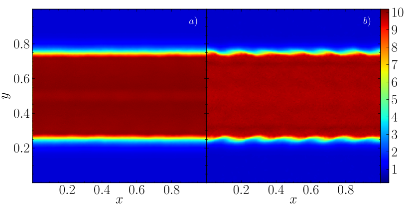
Figure 16: Shearing layer simulations at their respective $\tau_{\mathrm{KH}}$ using grid-based density smoothing. Left panel:$M=0.2$, using the LIQ kernel. Right panel: $M=0.4$, using the CS kernel. No improvement is seen over the column-based smoothing results.

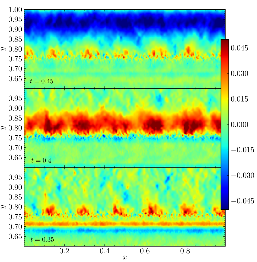
Figure 17: Rendered $v_{y}$ for a simulation with $M=0.2$, LIQ kernel, grid-based density smoothing. From bottom to top: $t=0.35,0.4,0.45$. Bottom panel: We see emerging KH instabilities as the 6 red $v_{y}$ areas around $y=0.75$. Below them, around $y=0.7$, we have a shock wave travelling upwards, with a small layer of positive $v_{y}$ in front of it and a region of negative $v_{y}$ in its wake. Middle panel: The shock is now almost at the same height of the instabilities. Its front is entering the low-density layer, increasing its $y$-length. Upper panel: The shock has passed through the instabilities. These now have a drastically reduced magnitude. The wake of the shock is still visible as the big blue band at the top of the panel.

4.5.1 Relaxing

Because we want to avoid any influence from shock waves, which we have shown are moving through the simulation box, we set up a simulation where we have first relaxed the initial conditions. The relaxing scheme we used is a default SPH simulation, with the PdV terms removed from the energy equation. The energy of particles is thus not allowed to change due to expansion/contraction, only due to artificial viscosity and conductivity. We use this scheme to stay as close as possible to the original energy profile.

We have relaxed run LIQ1. Two different runs were started from this relaxing run, the first starting from the relaxing run snapshot at $t=0.5$, the second from the $t=1.0$ snapshot. None of these simulations show any formation of KH rolls. Rendered views of $v_{y}$ are shown in respectively Figs. 18 and 19. In Fig 18. we can see that the magnitude of the shock (bottom panel, around $y=0.7$) is greatly reduced compared to the shock in Fig. 17. The emerging instabilities are also reduced in magnitude when compared to those in Fig. 17, due to the increased particle disorder and widening of the discontinuities. The small shock is sufficient to remove these smaller emerging instabilities. In Fig. 19 we can see that the magnitude of the KH seeds is very small. They do not develop and slowly fade away. This is the result of the long relaxing time which greatly diffuses the energy discontinuity and introduces too much particle disorder.

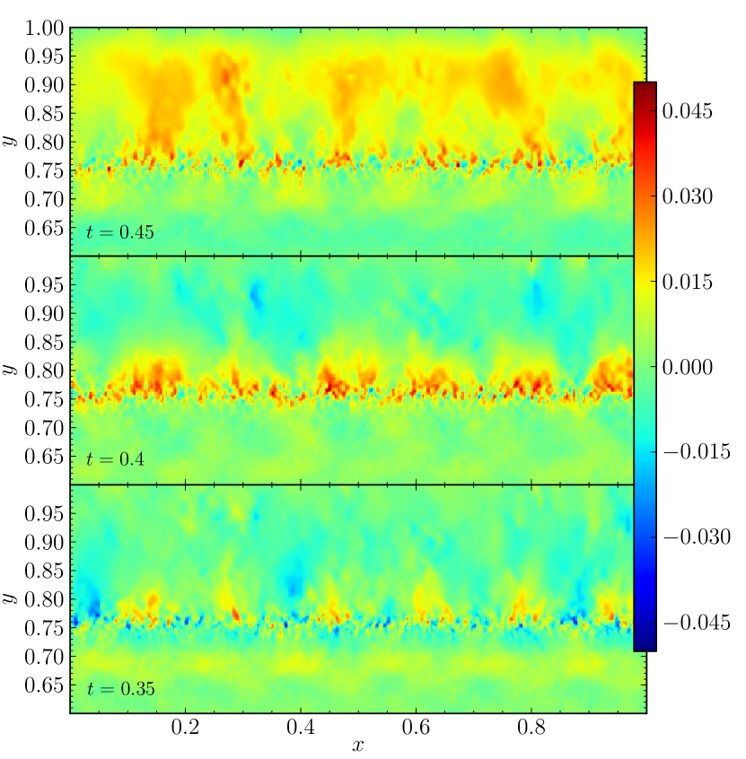
Figure 18: $M=0.2$ simulation starting from a LIQ1 IC which was relaxed during a time of $0.5$. From bottom to top: $t=0.35,0.4,0.45$ (after the end of relaxation). The same shock wave seen in Fig. 17 is present. However, its magnitude is greatly reduced, due to the relaxing of the IC. The initial KH seeds are also reduced in magnitude due to the increased particle disorder and general widening of the discontinuities.

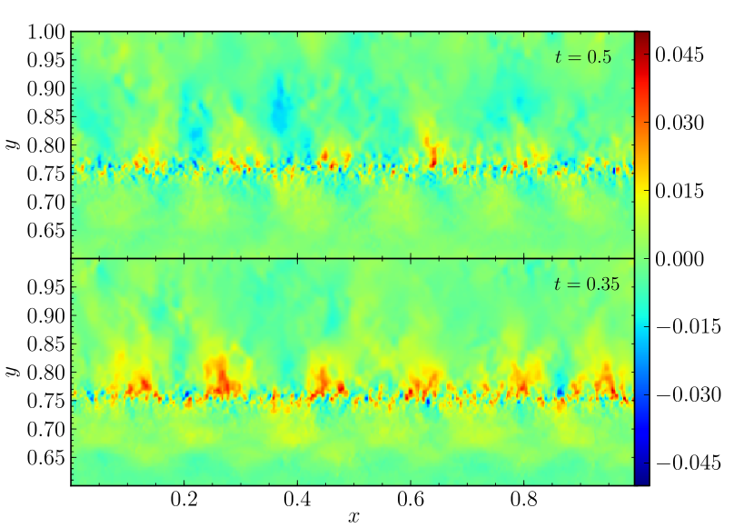
Figure 19: $M=0.2$ simulation starting from a LIQ1 IC which was relaxed during a time of $1$. Bottom panel: $t=0.35$ (after the end of relaxation). Top panel: $t=0.5$ (after relaxation). No shock is seen, the initial particle disorder and widening of the discontinuities themselves remove the growing KH instabilities.

4.6 Artificial Conductivity?

We have tested the need for artificial conductivity to be included in shearing layers simulations using the LIQ kernel and with an initially smoothed setup. To do this we repeated the LIQ1-5 simulations, with AC switched off. Results are shown in Fig. 20. The comparison with the bottom row of figure 10 learns us several things: i) applying artificial conductivity does not lead to the appearance of KH rolls. It is possible that with initial conditions which are not smooth and when using the CS kernel AC, provides an amount of smoothing in time for KHs to develop where they would not otherwise. ii) Artificial conductivity is needed to avoid an “oily” nature of the gas. iii) When comparing the long-term evolution of the simulations (Figs. 11 and 20), artificial conductivity in its default implementation is both a blessing and a curse. The panels in the bottom row of Fig. 20 show small-scale structures: “holes”, inclusions of low-density gas inside the high-density layer, are present in the high-density medium. When comparing with the grid-based simulations (Figs. 7 and 8) we see that these are also present there. In the simulation with AC applied these holes have entirely disappeared. It is however obvious that the tendency for the layers to avoid mixing without AC prevents realistic long-term behavior.

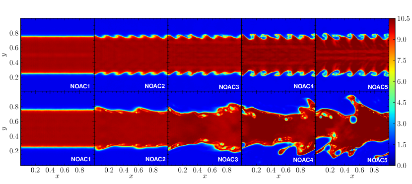
Figure 20: Shearing layers simulations without artificial conductivity (column-smoothed density). Left to right: Simulations NOAC1-NOAC5. Top row: simulations at their respective $\tau_{\mathrm{KH}}$. Bottom row: simulations at $t=2$.

4.6.1 Gap?

As recently highlighted by Agertz et al. (2007), SPH in its standard form (without AC) suffers from the formation of a “gap”, i.e. a small void layer between two layers with different densities. In Fig. 21 we show plots of two simulations without artificial conductivity, one with the CS kernel, the other with the LIQ kernel. It is clear that the LIQ kernel prevents the formation of a wide gap. As previously shown there still is a need for artificial conductivity (see Fig. 20) because the layers are still reluctant to mix. As we already achieved a great deal of improvement by trying one new smoothing kernel, we do not think it impossible that still better formulations are possible.

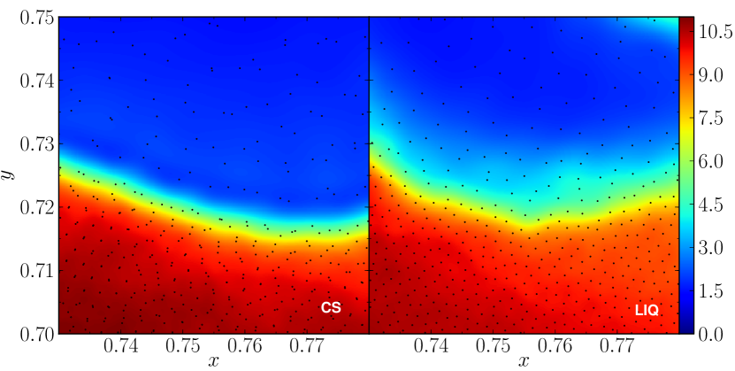
Figure 21: Density of two shearing layers simulations with $M=1$, at $\tau_{\mathrm{KH}}$, both without artificial conductivity. Left panel: Cubic spline kernel. Right panel: LIQ kernel. As previously shown the particle grouping of the CS kernel is abscent when using the LIQ kernel. Using the LIQ kernel also prevents the formation of a wide “gap” between the layers.

4.6.2 Signal velocity

In section 2.1 we briefly discussed the signal velocity used when including AC in simulations. In Fig. 22 we show some results using the modified signal velocities for simulations with $M=0.6$ and LIQ3 setup. They should thus be compared to panel m of Fig. 11. The top two rows show simulations using $v_{\mathrm{sig,1}}^{u}$ (eq. 5), the bottom two rows show results using $v_{\mathrm{sig,2}}^{u}$ (eq. 6). For both signal velocities, the results for $t=\tau_{\mathrm{KH}}$ are in good agreement with the grid simulation results as well as the other SPH results. At $t=2$ the results differ from the grid results, with the $\lambda=1/2$ clearly surfacing in the SPH simulations whereas this instability takes longer to surface in the grid results. When comparing with Fig. 11 it is obvious that for both signal velocities the amount of energy diffusion applied is smaller. Indeed, there is much more small-scale structure left in the $t=2$ panels in Fig. 22.

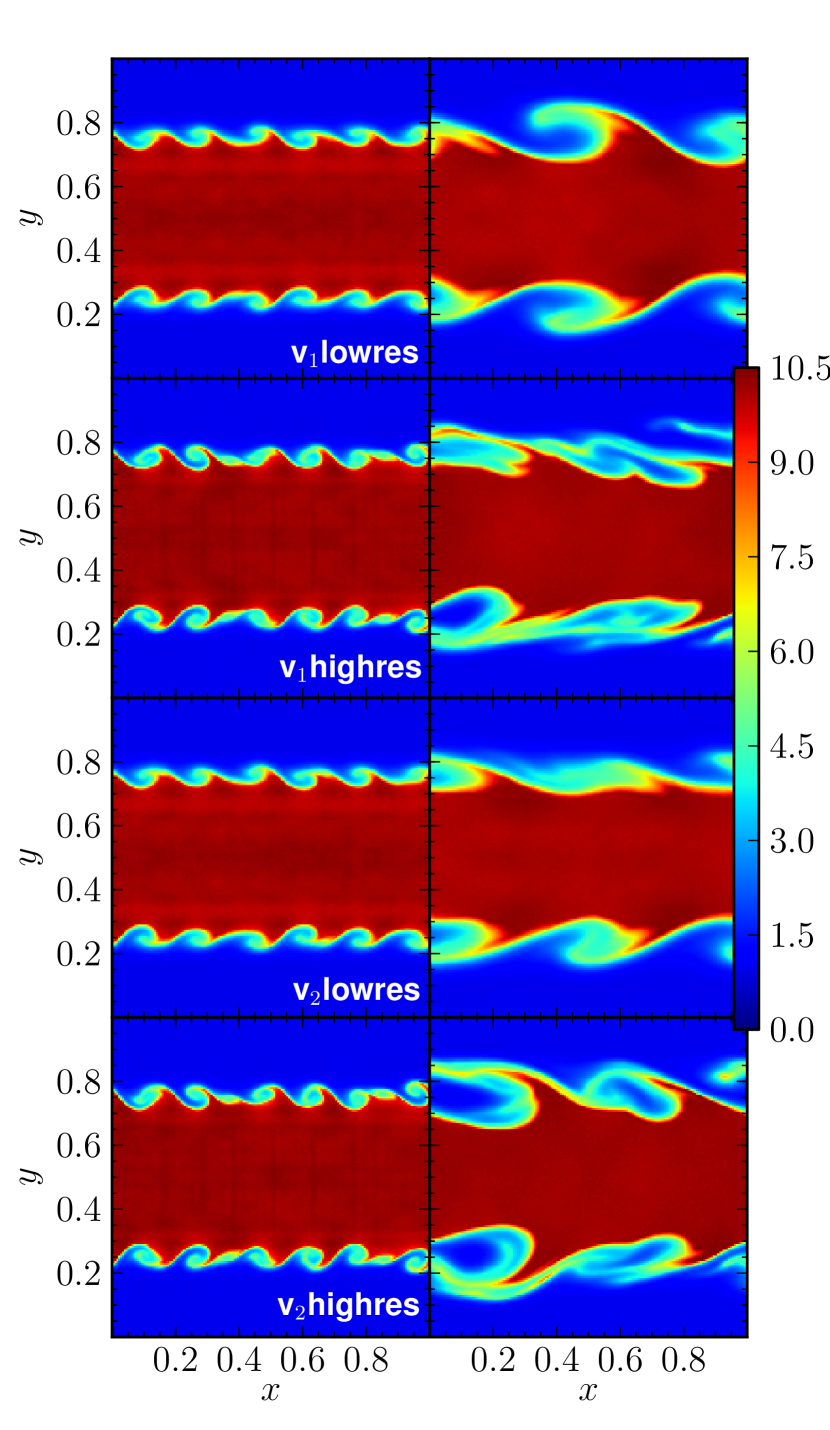
Figure 22: Density plots of shearing layers simulations with LIQ3 setup (see tables 3 and 4, $M=0.6$), using different signal velocities. Left column: $t=\tau_{\mathrm{KH}}$. Right column: $t=2$. Top two rows (label $v_{1}$): use the signal velocity from eq. (5). Bottom two rows (label $v_{2}$): use the signal velocity from eq. (6). lowres: 184 100 particles. highres: 552 100 particles.

We show a series of snapshots at different times in Fig. 23, in order to have a clear view of which instabilities are surfacing when. The top two rows (panels a-p) show the evolution of the LIQ3 simulation. It goes from $\lambda=1/6$ to $\lambda=1/2$ rolls, although the latter only appear on one side of the high-density layer. Panels q-F show a LIQ3 simulation with $v_{\mathrm{sig,1}}^{u}$ AC signal velocity (eq. (5)). Changing the sign of the signal velocity is a clear improvement in this case, with the KH rolls being even better resolved than in the LIQ3 simulation and with the rolls appearing on both sides of the central flow (see the grid simulation results in Fig. 8). Panels G-V show a LIQ3 simulation with $v_{\mathrm{sig,2}}^{u}$ signal velocity (eq. (6)). The KH rolls at $t=2$ are less well defined than in the LIQ3 simulation, they do appear on both sides of the flow. The result using $v_{\mathrm{sig,1}}^{u}$ thus compares favorably to the result using $v_{\mathrm{sig,2}}^{u}$ and using $v_{\mathrm{sig,1}}^{u}$ requires virtually no extra computations, as opposed to using $v_{\mathrm{sig,2}}^{u}$. It seems that using $v_{\mathrm{sig,1}}^{u}$ allows AC to act sufficiently strong to prevent clear layer separation (“oiliness” due to the LMI), but not too strong so as not to lose too much resolution by diffusing too much energy. Note that Fig. 22 shows that the actual results can change drastically when using a different resolution.

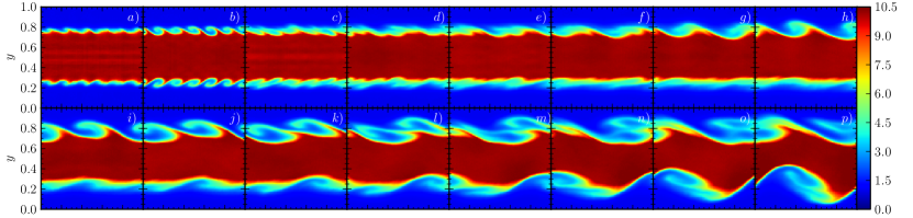
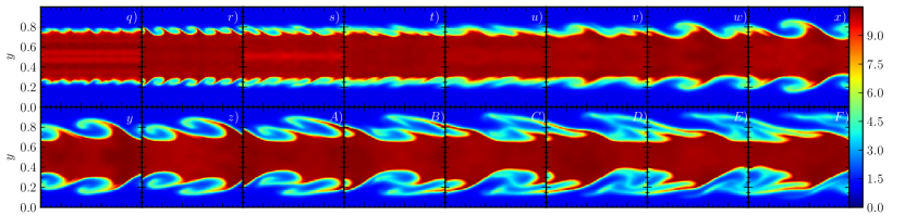
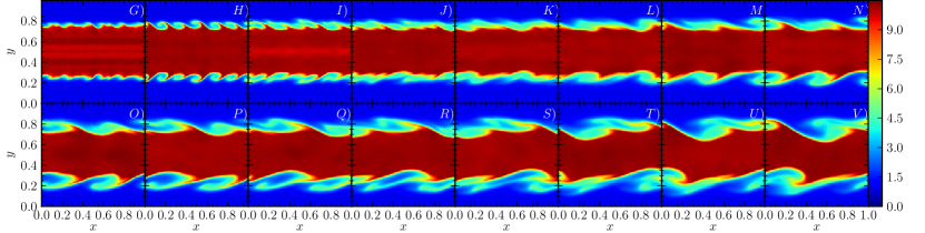
Figure 23: 16 snapshots of the density of 3 shearing layers simulations. Top rows (a-h, q-x, G-N): $t=0.25,0.5,0.75,1,1.25,1.5,1.75,2$, bottom rows (i-p, y-F, O-V): $t=2.25,2.5,2.75,3,3.25,3.5,3.75,4$. panels a-p: simulation LIQ3. panels q-F: simulation LIQ3 with modified AC signal velocity $v_{\mathrm{sig,1}}^{u}$ (see also Fig. 22, v₁lowres). This simulation develops clearly resolved $\lambda=1/2$ KH rolls. panels G-V: simulation LIQ3 with modified AC signal velocity $v_{\mathrm{sig,2}}^{u}$ (see also Fig. 22, v₂lowres). This develops less well defined $\lambda=1/2$ KH rolls, these do appear on both sides of the central stream, contrary to the LIQ3 simulation.

5 Discussion

Using a large suite of simulations we have shown that the performance of SPH on the shearing layers test can be improved drastically, if i) the density gradient in the initial conditions is smoothed and ii) a smoothing kernel that does not cause particle clumping is used. Two effects are in play that can cause things to go haywire: shocks travelling through the simulation box and particle clumping, or more general, particle disorder. The effect of SPH particle disorder was already discovered by Okamoto et al. (2003), who set up a simulation with a small, hot shearing flow layer inside a cold medium. They found that noisiness in the SPH smoothing of variables gives rise to small-scale pressure gradients which significantly decelerated the shearing flow. As using the Cubic Spline smoothing kernel causes particles to clump together in groups of 2, as can be seen in the left panel of Fig. 21, we can expect deceleration of SPH particles located in a small layer around the contact interface. This layer then acts as a lubricant between the two shearing layers, removing direct contact of the latter two and hence preventing KH instabilities from forming or growing. The LIQ kernel on the other hand gives rise to a much more homogeneous particle distribution (right panel of Fig. 21). Employing a suitble smoothing kernel with non-zero central first derivative (we say suitable because although the first derivative being non-zero is necessary to avoid clumping, it is not sufficient: a LIQ kernel with connection point $x_{\mathrm{s}}=0.5$ suffers from even heavier clumping than the CS kernel: particles tend to clump together in groups of 6) gives rise to a much more homogeneous particle distribution. This has a major impact on shearing layers simulations, allowing KHIs to form much easier in general. The effect of particle disorder has been highlighted in the literature on various occasions. Read et al. (2010) show that particle clumping gives a large E0 error in the SPH momentum equation, which in turn prevents mixing in SPH. Morris (1996) also found that that SPH does not converge at flow boundaries because of the E0 error.

The shock problem is not so easily tackled. The shocks are triggered by the local mixing instability, which occurs because energy (entropy) is not smoothed in SPH. Several authors have identified this problem (e.g. Cummins & Rudman, 1999; Tartakovsky & Meakin, 2005; Agertz et al., 2007; Price, 2008; Read et al., 2010) and various solutions have been suggested. We examined the results using the artificial conductivity solution (Price, 2008). The magnitude of the shock-waves can be reduced by applying an initial density smoothing, which reduces the magnitude of any shock waves that might develop, leading to a significant increase in the simulation results. To get rid of the remaining shocks one can relax a simulation before applying velocities to it. This does not help in this case however because relaxing not only significantly widens the density and energy discontinuities, it also removes a great deal of the symmetry that was initially present in the problem, i.e. it introduces a lot of particle disorder. Indeed, a simulation started from a grid has perfect initial particle symmetry and as sharp a discontinuity as one desires. When relaxing the initial conditions on the other hand, particle positions are shifted to reach an equilibrium. The smoothing kernel plays an important part in this because through small-scale variations in forces it will determine the final configuration of the particles. This can readily be seen in Fig. 5. Even when using the LIQ kernel there is an increased amount of particle noise. When bulk shearing layers velocities are then given to particles based on on which side of a line they lay, and velocity perturbations applied to particles irrespective of the underlying configuration of the particles, it is not hard to imagine that the problem of the particle noise will quickly result in momentum transfer at the contact layers, thus shutting down all KH-related activities. Furthermore, we found that the onset of the shock-waves, occuring because of the LMI triggered in the initial particle configuration, is not removed by the artificial conductivity.

We found that adding artificial conductivity to the SPH scheme does not have an impact on whether or not initial ($\lambda=1/6$) KHIs surface. Although it has been reported and used as such in the literature (see e.g. Price, 2008; Kawata et al., 2009) we show that simulations that use a suitable smoothing kernel and a smoothed initial density gradient are equally able to form these KHIs, irrespective of AC being included or not. Even the formation of a visible “gap” (Agertz et al., 2007) is prevented by using a suitable smoothing kernel (Fig. 21). Including AC is, with the smoothing kernels used in this paper, still necessary to i) allow mixing to happen, avoiding “oily” features in the SPH gas phases (see Fig. 20) and preventing the LMI from triggering during the course of the simulation and ii) get the $\lambda=1/2$ KH rolls later on. Here, point ii) might very well be a consequence of point i). We find that it is easy to actually lose substructure that was initially resolved in SPH because of superfluous energy diffusion (see Figs. 11, 20 and 22). When using SPH to solve very sensitive hydrodynamical problems (like the current shearing layers problem) one should therefore take good care when including the artificial conductivity and in selecting an appropriate signal velocity. We presented two new signal velocities to that effect: $v_{\mathrm{sig,1}}^{u}$ (eq. (5)) and $v_{\mathrm{sig,2}}^{u}$ (eq. (6)). Shearing layers results indicate that both these signal velocities lead to less energy diffusion in simulations. $v_{\mathrm{sig,1}}^{u}$ emerges as the best choice, giving better results in terms of KH rolls and requiring no significant extra computations.

The combined effect of both the shock waves and the particle disorder becomes less and less important as the time-scale of the problem itself (in this case: $\tau_{\mathrm{KH}}$) decreases. At he resolution of current galaxy formation simulations mixing is probably not important. However, mixing could become crucial for next-generation simulations. Also, for the standard astrophysical application the actual choice of AC sigal velocity will be less of a concern, if a concern at all, as is demonstrated by the host of successful problems tackled by the SPH codes of Rosswog & Price (2007) and Kawata et al. (2009). Note that a suitable signal velocity for simulations including gravity has not as of yet been presented.

Appendix A LIQ kernel coefficients

The expressions for the parameters of the LIQ kernel (eq. (9)), obtained by solving the set of equations (10a–10f), are:

$$\alpha = \frac{1}{x_{\mathrm{s}}^{3}-3x_{\mathrm{s}}^{2}+3x_{\mathrm{s}}-1}$$ (23)

$$A = \frac{\alpha}{2}$$ (24)

$$B = -\alpha(1+x_{\mathrm{s}})$$ (25)

$$C = 3\alpha x_{\mathrm{s}}$$ (26)

$$D = -\alpha(-1+3x_{\mathrm{s}})$$ (27)

$$E = \frac{\alpha(2x_{\mathrm{s}}-1)}{2}$$ (28)

$$F = Ax_{\mathrm{s}}^{4}+Bx_{\mathrm{s}}^{3}+Cx_{\mathrm{s}}^{2}+Dx_{\mathrm{s}}+E+x_{\mathrm{s}},$$ (29)

with $x_{\mathrm{s}}$ the LIQ kernel connection point. From this it is straightforward to calculate the norm $N$ by integrating over the volume:

$$N=\left[\int_{0}^{x_{\mathrm{s}}}W_{r}(u)\mathrm{d}u+\int_{x_{\mathrm{s}}}^{1}W_{r}(u)\mathrm{d}u\right]^{-1}.$$ (30)

Calculating $N$ is then straightforward. We give the expressions here for completeness. In two dimensions:

$$\int_{0}^{x_{\mathrm{s}}}W_{r}(u)\mathrm{d}u =2\pi\left(\frac{1}{2}Fx_{\mathrm{s}}^{2}-\frac{1}{3}x_{\mathrm{s}}^{3}\right)$$ (31)

$$\int_{x_{\mathrm{s}}}^{1}W_{r}(u)\mathrm{d}u =2\pi\Big{(}\frac{A}{6}x_{\mathrm{s}}^{6}+\frac{B}{5}x_{\mathrm{s}}^{5}+\frac{C}{4}x_{\mathrm{s}}^{4}$$ (32)

$$\qquad\qquad\qquad+\frac{D}{3}x_{\mathrm{s}}^{3}+\frac{E}{2}x_{\mathrm{s}}^{2}\Big{)}\Big{|}_{x_{\mathrm{s}}}^{1}.$$ (33)

In three dimensions:

$$\int_{0}^{x_{\mathrm{s}}}W_{r}(u)\mathrm{d}u =4\pi\left(\frac{1}{3}Fx_{\mathrm{s}}^{3}-\frac{1}{4}x_{\mathrm{s}}^{4}\right)$$ (34)

$$\int_{x_{\mathrm{s}}}^{1}W_{r}(u)\mathrm{d}u =4\pi\Big{(}\frac{A}{7}x_{\mathrm{s}}^{7}+\frac{B}{6}x_{\mathrm{s}}^{6}+\frac{C}{5}x_{\mathrm{s}}^{5}$$ (35)

$$\qquad\qquad\qquad+\frac{D}{4}x_{\mathrm{s}}^{4}+\frac{E}{3}x_{\mathrm{s}}^{3}\Big{)}\Big{|}_{x_{\mathrm{s}}}^{1}.$$ (36)

References

- Agertz et al. (2007) Agertz O., Moore B., Stadel J., Potter D., Miniati F., Read J., Mayer L., Gawryszczak A., Kravtsov A., Nordlund Å., Pearce F., Quilis V., Rudd D., Springel V., Stone J., Tasker E., Teyssier R., Wadsley J., Walder R., 2007, MNRAS, 380, 963
- Chandrasekhar (1961) Chandrasekhar S., 1961, Hydrodynamic and hydromagnetic stability
- Cummins & Rudman (1999) Cummins S. J., Rudman M., 1999, Journal of Computational Physics, 152, 584
- Dubey et al. (2008) Dubey A., Reid L. B., Fisher R., 2008, Physica Scripta, T132, 014046
- Fryxell et al. (2000) Fryxell B., Olson K., Ricker P., Timmes F. X., Zingale M., Lamb D. Q., MacNeice P., Rosner R., Truran J. W., Tufo H., 2000, ApJSS, 131, 273
- Fulk (1996) Fulk D., 1996, Journal of Computational Physics, 126, 165
- Gingold & Monaghan (1977) Gingold R. A., Monaghan J. J., 1977, MNRAS, 181, 375
- Hess & Springel (2009) Hess S., Springel V., 2009, ArXiv e-prints
- Hu & Adams (2009) Hu X. Y., Adams N. A., 2009, Journal of Computational Physics, 228, 2082
- Johnson et al. (1996) Johnson G. R., Stryk R. A., Beissel S. R., 1996, Computer Methods in Applied Mechanics and Engineering, 139, 347
- Kawata et al. (2009) Kawata D., Okamoto T., Cen R., Gibson B. K., 2009, ArXiv e-prints
- Lucy (1977) Lucy L. B., 1977, AJ, 82, 1013
- Merlin et al. (2009) Merlin E., Buonomo U., Grassi T., Piovan L., Chiosi C., 2009, ArXiv e-prints
- Monaghan (1997) Monaghan J. J., 1997, Journal of Computational Physics, 136, 298
- Monaghan (2000) Monaghan J. J., 2000, Journal of Computational Physics, 159, 290
- Morris (1996) Morris J. P., 1996, Publications of the Astronomical Society of Australia, 13, 97
- Okamoto et al. (2003) Okamoto T., Jenkins A., Eke V. R., Quilis V., Frenk C. S., 2003, MNRAS, 345, 429
- Price (2005) Price D., 2005, ArXiv Astrophysics e-prints
- Price (2008) Price D. J., 2008, Journal of Computational Physics, 227, 10040
- Read et al. (2010) Read J. I., Hayfield T., Agertz O., 2010, MNRAS, pp 767–+
- Robertson et al. (2010) Robertson B. E., Kravtsov A. V., Gnedin N. Y., Abel T., Rudd D. H., 2010, MNRAS, 401, 2463
- Rosswog & Price (2007) Rosswog S., Price D., 2007, MNRAS, 379, 915
- Schuessler & Schmitt (1981) Schuessler I., Schmitt D., 1981, A&A, 97, 373
- Sigalotti et al. (2009) Sigalotti L. D. G., López H., Trujillo L., 2009, Journal of Computational Physics, 228, 5888
- Sod (1978) Sod G. A., 1978, Journal of Computational Physics, 27, 1
- Springel (2005) Springel V., 2005, MNRAS, 364, 1105
- Springel & Hernquist (2002) Springel V., Hernquist L., 2002, MNRAS, 333, 649
- Tartakovsky & Meakin (2005) Tartakovsky A. M., Meakin P., 2005, Journal of Computational Physics, 207, 610
- Tasker et al. (2008) Tasker E. J., Brunino R., Mitchell N. L., Michielsen D., Hopton S., Pearce F. R., Bryan G. L., Theuns T., 2008, MNRAS, 390, 1267
- Thomas & Couchman (1992) Thomas P. A., Couchman H. M. P., 1992, MNRAS, 257, 11
- Vanaverbeke et al. (2009) Vanaverbeke S., Keppens R., Poedts S., Boffin H., 2009, Computer Physics Communications, 180, 1164