Vortices in quantum droplets: Analogies between boson and fermion systems

Abstract

The main theme of this review is the many-body physics of vortices in quantum droplets of bosons or fermions, in the limit of small particle numbers. Systems of interest include cold atoms in traps as well as electrons confined in quantum dots. When set to rotate, these in principle very different quantum systems show remarkable analogies. The topics reviewed include the structure of the finite rotating many-body state, universality of vortex formation and localization of vortices in both bosonic and fermionic systems, and the emergence of particle-vortex composites in the quantum Hall regime. An overview of the computational many-body techniques sets focus on the configuration interaction and density-functional methods. Studies of quantum droplets with one or several particle components, where vortices as well as coreless vortices may occur, are reviewed, and theoretical as well as experimental challenges are discussed.

I Introduction

In recent years, advances in experimental methods in quantum optics as well as semiconductor physics have made it possible to create confined quantum droplets of particles, and to manipulate them with unprecedented control. Bose-Einstein condensates of ultra-cold atomic gases, for example, may be set rotating either by rotating the trap, or by “stirring” the cold atoms with lasers. These clouds of bosons are large in present day experiments, but the regime of few-particle bosonic droplets ultimately may be reached. Confined electron droplets, on the other hand, are nowadays routinely realized as low-dimensional nanostructured quantum dots in semiconductors, where the droplet size and its angular momentum can be accurately fixed by an external voltage bias and a magnetic field, respectively. A bosonic atom cloud in a trap, and electrons confined in quantum dots are very different systems by nature. However, when set to rotate, their microscopic properties show remarkable analogies. While quantum dots are usually quasi-two-dimensional due to the semiconductor heterostructure, the dimensionality is reduced also in a trapped rapidly rotating atom gas due to the centrifugal force, which flattens the cloud of atoms.

The structure of a quantum state describing a rotating droplet fundamentally reflects how the system carries angular momentum. Intriguingly, some of the underlying mechanisms appear universal in two-dimensional systems regardless of the particle statistics, wave function symmetries, and the form of the interparticle interaction. For example, both bosonic and fermionic droplets show formation of vortices in the droplet with increasing angular momentum. Eventually, in the regime of very rapid rotation, finite-size precursors of fractional quantum Hall states with particle-vortex composites are predicted to emerge similarly in both bosonic and fermionic systems. Due to these universalities in the structure of the quasi-two-dimensional many-body state, rotating quantum droplets can often be described theoretically by similar concepts and analogous vocabulary. These analogies are the main theme of this review, where boson and fermion systems are treated in parallel and similarities and differences between these systems are extensively discussed.

Despite the close connection between rotating cold atom gases and electrons in nanostructured quantum systems in solids, research efforts in these fields have advanced mostly independently of each other. In this review we highlight the similarities between these fields, with the hope that it may serve as a source of inspiration for further studies on rotating quantum systems where complex and sometimes unexpected phenomena emerge.

I.1 Finite quantum liquids in traps

Confining elementary particles or indistinguishable composite particles, such as atoms, by cavities or external potentials at low temperatures, one may create finite-size quantum systems with particle numbers ranging from just a few to millions. Cold atomic quantum gases in traps and lattices, photons in cavities and electrons confined in low-dimensional semiconductor nanostructures are well-known examples.

I.1.1 Atoms in traps

Bose and Einstein predicted already in the 1920s the condensation of an ideal gas of bosonic particles into a single, coherent quantum state Bose (1924); Einstein (1925, 1924). Apart from strongly interacting systems such as liquid helium, the experimental discovery of this phenomenon had to wait many decades, until advances in cooling and trapping techniques for dilute atomic gases finally made possible the observation of Bose-Einstein condensation (BEC) in a cloud of cold bosonic alkali atoms Anderson et al. (1995); Davis et al. (1995a, b); Ensher et al. (1996); Ketterle (2002); Cornell and Wieman (2002). These celebrated experiments clearly marked a new era in quantum physics combining the fields of quantum optics, condensed matter physics and atomic physics. For the physics of BEC, see for example the review article by Leggett (2001) as well as Dalfovo et al. (1999), the monographs by  Pethick and Smith (2002); Leggett (2006); Pitaevskii and Stringari (2003), and Inguscio et al. (1999).

A BEC can be set rotating not only by rotating the trap, but also by stirring the bosonic droplet with lasers Madison et al. (2000, 2001); Chevy et al. (2000); Abo-Shaer et al. (2001), or by evaporating atoms Haljan et al. (2001); Engels et al. (2002, 2003) (see the discussion in the recent review by Fetter (2009)). A weakly interacting dilute system becomes effectively two-dimensional when set rotating, making a description in the lowest Landau level possible. We mainly restrict our analysis of BEC’s in this review to this limit of quasi-two-dimensional droplets of atoms.

More recently, superfluid states have been realized also for trapped fermionic atoms, where fermion pairing or molecule formation can occur in two distinct regimes depending on the atomic interaction strength. Pairing can take place in real space via molecule formation and these composite bosons may then show Bose-Einstein condensation Greiner et al. (2003); Jochim et al. (2003); Regal et al. (2004); Zwierlein et al. (2004). Pairing can also occur in momentum space via formation of correlated Cooper pairs and the superfluid state would be analogous to the Bardeen-Cooper-Schrieffer (BCS)-type of a superconducting state Zwierlein et al. (2005); Chin et al. (2006). This is a relatively novel field and not treated here; part of it has been reviewed by Giorgini et al. (2008) and Bloch et al. (2008).

I.1.2 Electrons in low-dimensional quantum dots

Quantum dots are man-made nanoscale droplets of electrons trapped in all spatial directions. As they show typical properties of atomic systems, such as shell structure and discrete energy levels, they are often referred to as artificial atoms Ashoori (1996). Electron numbers in quantum dots may reach thousands. Quantum dots are often fabricated in semiconductor materials, but the use of graphene has also been proposed Trauzettel et al. (2007); Wunsch et al. (2008). These nanostructured finite fermion systems have been studied extensively for (by now) two decades. Several review articles, discussing the quantum transport through quantum dots van der Wiel et al. (2003), electronic structure Reimann and Manninen (2002), the role of symmetry breaking and correlation Yannouleas and Landman (2007) as well as spin in connection with quantum computing Coish and Loss (2007); Cerletti et al. (2005); Hanson et al. (2007), were published.

The semiconductor quantum dots discussed here are of either lateral or vertical type. In a lateral device the electrons in a two-dimensional electron gas are trapped by external electrodes, while vertical dots are formed by, e.g., etching out a pillar from a wafer containing a heterostructure. In both cases the motion of electrons is restricted into a thin disk, with a typical radius of few tens up to hundred nanometers, and a thickness that is often an order of magnitude smaller. Electrons in quantum dots can be set rotating by external magnetic fields perpendicular to the plane of motion. Other stirring mechanisms have also been proposed, e.g. rotation in the electric field of laser pulses Räsänen et al. (2007). Due to the band structure of the underlying semiconductor material, magnetic field strengths giving rise to transitions in the electronic structure of quantum dots are orders of magnitude lower than in real atomic systems, and attainable in laboratories. Much of the information about the electronic structure must be extracted from electron transport measurements Oosterkamp et al. (1999). Direct imaging methods of electron densities in quantum dots have also been attempted, see for example Fallahi et al. (2005); Dial et al. (2007), but not yet proven equally useful in this context.

Quantum dots in external magnetic fields have a very close connection to quantum Hall systems, the only difference being that the quantum Hall effect is measured in a sample of the two-dimensional electron gas (2DEG), which is often modeled as an infinite system. Quantum dots, however, are finite-size many-body systems. At strong magnetic fields, where electrons occupy only the lowest Landau level, they are thus often referred to as “quantum Hall droplets” Oaknin et al. (1995); Yang and MacDonald (2002). Many concepts familiar from the theory of the quantum Hall effect, such as the Landau level filling factor, can be generalized for these finite-size droplets Kinaret et al. (1992); Reimann and Manninen (2002). However, due to the presence of the external confining potential in quantum dots, the analogy to quantum Hall states in the infinite 2DEG is not exact and edge effects play an important role Viefers (2008); Cooper (2008).

I.2 Vortex formation in rotating quantum liquids

The formation of vortices in a liquid that is set to rotate is often a result of turbulent flow. In the epic poem “The Odyssey”, Homer describes Ulysses’ encounter with Charybdis, a monster-goddess who sucked sea water and created a giant whirlpool Homer (8th century B.C.). This early account of vortex dynamics is strikingly accurate in identifying the characteristics of vortices, namely, the rotating current of the whirlpool and the cavity at the center of the vortex which engulfed the ships sailing nearby. Homer’s description may well be illustrated by other examples of more harmless vortices, such as whirlpools in bathtubs where water is draining out Andersen et al. (2003). Other well-known examples of vortices in air include tornadoes, or wake vortices created by an airplane wing (Figs.1(a) and (b)).

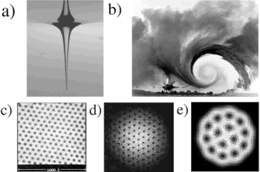
Figure 1: Examples of vortices and vortex lattices. Vortices are ubiquitous in both classical and quantum systems: a) classical whirlpool vortex Andersen et al. (2003), b) wake vortex of a passing airplane wing, revealed by colored smoke (NASA Langley Research Center, Figure ID: EL-1996-00130) c) STM-image of an Abrikosov vortex lattice Abrikosov (1957) in a type-II superconductor Hess et al. (1989), d) vortex lattice in a rotating Bose-Einstein condensate of ⁸⁷Rb atoms (adapted from Coddington et al. (2004)), e) cluster of vortices in the calculated electron density of a 24-electron quantum dot, after Saarikoski et al. (2004). In panels c)-e), the vortices appear as “holes” in the particle density.

Vortices are ubiquitous also in quantum mechanical systems under rotation (see Figs. 1(c)-(e)). It is well known that the magnetic field in type-II superconductors penetrates through vortex lines Tinkham (2004) (see Fig. 1(c)). Superfluid ⁴He is another example where vortices may form in a strongly interacting bosonic quantum fluid Williams and Packard (1974); Yarmchuk et al. (1979); Yarmchuk and Packard (1982). (See also the early work by Onsager (1949), London (1954) and Feynman (1955), and for example the book by Donnelly (1991).) Vortices appear as a very general phenomenon in Bose as well as in Fermi systems with high as well as low particle density. They may emerge for short-range interactions between the particles, as in condensates of neutral atoms (as shown in Fig. 1(d) for a rotating Bose-Einstein condensate of ⁸⁷Rb atoms) or – perhaps more surprisingly – even in electron systems with long-range Coulomb repulsion, see Fig. 1(d) showing the vortices in a quantum dot at a strong magnetic field.

I.2.1 Vortices in Bose-Einstein Condensates

For vortices in rotating Bose-Einstein condensates, early theoretical descriptions have set focus on the Thomas-Fermi regime of strong interactions, see for example Rokhsar (1997); García-Ripoll and Pérez-García (1999); Feder et al. (1999a, b); Svidzinsky and Fetter (2000), as well as weak interactions Mottelson (1999); Butts and Rokhsar (1999); Kavoulakis et al. (2000). Baym and Pethick (1996) treated vortex lines in terms of the Gross-Pitaevskii approach, and later on also discussed the transition to the lowest Landau level when the rotation rate was increased Baym and Pethick (2004).

Intense experimental research efforts were made to observe vortices in rotating clouds of bosonic atoms, see e.g., the early experimental work by Matthews et al. (1999), as well as Madison et al. (2000), Abo-Shaer et al. (2001), Engels et al. (2002, 2003), and Schweikhard et al. (2004). For recent reviews, we refer to the articles by Fetter (2009), as well as  Bloch et al. (2008).

In weakly interacting and dilute systems, an effective reduction of dimensionality can for example be caused by rotation as a simple consequence of the increase in angular momentum. Due to the reduction in dimensionality, phase singularities, i.e., nodes in the wave functions, become important.

With increasing angular momentum, one finds successive transitions between patterns of singly-quantized vortices, arranged in regular arrays. In finite-size systems, so-called “vortex molecules” are formed, in much analogy to finite-size superconductors Milosevic and Peeters (2003).

There exist many analogies of a rotating cloud of bosonic atoms with (fractional) quantum Hall physics Wilkin et al. (1998); Cooper and Wilkin (1999); Viefers et al. (2000); Ho (2001). This in fact may also give important theoretical insights into the regime of extreme rotation which has not yet been achieved experimentally. (For related reviews, see Cooper (2008); Viefers (2008) and Fetter (2009)).

I.2.2 Vortices in quantum Hall droplets

Vortices have been an integral part of the theory of quantum Hall states in the 2D electron gas since the proposal of the Laughlin state Laughlin (1983). They emerge also in quantum dots Saarikoski et al. (2004); Toreblad et al. (2004) at strong magnetic fields, and close connections of these vortices to those that can be found in rotating bosonic systems have been established Toreblad et al. (2004, 2006); Manninen et al. (2005); Borgh et al. (2008). The vortex patterns in quantum dots depend on the strength of the external magnetic field, and on intricate details of particle interactions Saarikoski et al. (2004); Tavernier et al. (2004).

In the regime of slow rotation, vortices (except those originating from the Pauli principle) are not bound to particles and form charge deficiencies in the density distribution, which may localize to structures in the particle and current densities that resemble the aforementioned vortex molecules or regular vortex arrays in rotating Bose-Einstein condensates Saarikoski et al. (2004, 2005b); Manninen et al. (2005). The emergence of vortices that carry the angular momentum of the droplet is manifest in the structure of the many-body states. For fermions they may be described as hole-like quasiparticles Manninen et al. (2005). When the number of vortices increases with the angular momentum, the electrons and vortices may form composites well known from the theory of the fractional quantum Hall effect, see for example Jain (1989) or Viefers (2008).

I.2.3 Quantum Hall regime in bosonic condensates

In quantum dots, the fractional quantum Hall regime with a high vortex density can be readily attained at high magnetic fields. For the case of rotating cold atom condensates, despite extensive experimental studies Coddington et al. (2003); Schweikhard et al. (2004), this regime of extreme rotation is not yet within easy reach. Very recently, however, it was suggested to exploit the equivalence of the Lorentz and the Coriolis force to realize “synthetic” magnetic fields in rotating neutral systems, which could be a very important step forward in the efforts to realize BEC’s at extreme rotation Lin et al. (2009). To date, experiments with rotating BEC’s are only able to access states where the number of vortices is relatively small compared to the number of particles Matthews et al. (1999); Madison et al. (2000); Abo-Shaer et al. (2001); Engels et al. (2002, 2003); Schweikhard et al. (2004); Fetter (2009). A high vortex density creates a highly correlated state. Counterparts of typical quantum Hall states, such as the bosonic Laughlin state and other incompressible states, as well as states having non-Abelian particle excitations, are predicted to emerge Wilkin et al. (1998); Cooper and Wilkin (1999); Viefers (2008); Lin et al. (2009). Compared to the quantum Hall systems in the 2D electron gas, rotating cold-atom condensates offer a high level of tunability since particle interactions and trap geometries can be easily modified. This makes bosonic quantum Hall states an extremely interesting field of research Viefers (2008); Cooper (2008).

I.2.4 Self-bound droplets

A common feature of all the systems discussed above is that the particles are bound by an external confinement, which often can be approximated to be harmonic. Nuclei, helium droplets and atomic clusters provide other interesting finite quantum systems where rotational states have been studied. These systems are self-bound due to attractive interactions between (at least some of) the components.

Rotational states, shape deformations and fission of self-bound droplets are interesting topics in their own right. However, while in a harmonic confinement the fast rotation causes the droplet to flatten into a quasi-two-dimensional circular disk, this is usually not the case in self-bound clusters, where the rotation can be accompanied with a noncircular deformation, often a two-lobed or even more complicated shape Hill and Eaves (2008). Eventually this can lead to a fission of the droplet to smaller fragments, preventing the occurrence of very large angular momenta and vortex formation. In the case of nuclei, the rotational spectrum is usually related to deformation Bohr and Mottelson (1975). Nevertheless, the possibility of vortex-like excitations has also been discussed, see Fowler et al. (1985), and nuclear matter is expected to carry vortices in neutron stars Baym et al. (1969); Link (2003).

The only small self-bound system where vortices are likely to occur, is a helium droplet. Grisenti and Toennies (2003) indicate that anomalies in their cluster beam experiments could be caused by vortex formation. However, no clear experimental evidence of vortex formation in small helium droplets has yet emerged, while theoretical studies suggest that vortices form in ⁴He nanodroplets Mayol et al. (2001); Lehmann and Schmied (2003); Sola et al. (2007). The properties of helium nanodroplets have been recently reviewed by Barranco et al. (2006).

I.3 About this review

The main concern of this review are the structural properties of the many-body states of small two-dimensional quantum droplets, where rotation induces strong correlations and vortex formation. The direct connections between bosonic and fermionic systems, as well as finite-size quantum droplets and infinite quantum Hall systems are recurrent themes. Other reviews complement our work by taking different approaches: We refer to Fetter (2009) for a review of rotating BEC’s especially in the regime which is accessible with present day experimental setups, and to Viefers (2008) for a review which focuses on the quantum Hall physics in rotating BEC’s. Another recent review by  Cooper (2008) describes rotating atomic gases in both the mean-field and the strongly correlated regimes. A review on the many-body phenomena and correlations in dilute ultra-cold gases that also discusses rotation, was recently published by Bloch et al. (2008).

Quantum dot physics is a versatile field. We refer to Reimann and Manninen (2002) and Yannouleas and Landman (2007), as well as van der Wiel et al. (2003) and Hanson et al. (2007) for reviews on the electronic structure and spin-related phenomena. Vortices in superconducting quantum dots have also been much discussed in the literature, but are not treated here. We instead refer the reader for example to the more recent articles by  Baelus et al. (2001), Baelus and Peeters (2002), Baelus et al. (2004) and Grigorieva et al. (2006).

We begin this review in Sec. II by introducing basic concepts to characterize the many-body states of rotating systems. Section III discusses some of the computational many-body methods used. Section IV discusses vortex formation in rotating quantum liquids which are composed of one type of particles (or one spin component), while Section V is concerned with coreless vortices in multi-component systems. We conclude the review and discuss possible future challenges in Sec. VI.

(Unless stated otherwise, equations are presented in SI units whereas most results of calculations are in atomic units.)

II Many-body wave function

In the following, we briefly describe concepts and methods to analyze the internal structure of the many-body states, such as pair-correlation functions and conditional probabilities. We then proceed to show the connections between boson and fermion states, and particle-hole duality that treats vortices as hole-like quasi-particles. We finally give a brief overview of the connections to the quantum Hall physics in the (infinite) two-dimensional electron gas.

II.1 Model Hamiltonian

II.1.1 Rotating quantum droplets of bosons

Clouds of bosonic condensates are usually confined by a harmonic trap that extends in all three spatial dimensions. An axisymmetric rotation with frequency $\Omega$ leads to centrifugal forces which flatten the density by extending the radial size of the system, while the cloud contracts in the axial direction. The ratio between the axial thickness $R_{z}$ and radial thickness $R_{\perp}$ of the rotating cloud, i.e., the aspect ratio, can be calculated within the Thomas-Fermi approximation Fetter (2009)

$${R_{z}\over R_{\perp}}={\sqrt{\omega_{\perp}^{2}-\Omega^{2}}\over\omega_{z}},$$ (1)

where $\omega_{z}$ and $\omega_{\perp}$ are the radial and axial trapping frequencies, respectively. Imaging of the condensate Raman et al. (2001); Schweikhard et al. (2004) confirms that the rotation reduces the aspect ratio effectively.

With the trap rotating at an angular velocity $\Omega$, in the laboratory frame of reference the problem is time-dependent. One thus conveniently introduces a rotating frame at the angular velocity $\Omega$, in which the (now time-independent) Hamiltonian contains an extra inertial term $-\Omega{\bf L}$, where ${\bf L}$ is the total angular momentum operator.

In the case of circular symmetry of the 2D system, for its rotation around the $z$-axis, the angular momentum operator $L=L_{z}$ commutes with the Hamiltonian. We may write

$$H_{\Omega}=H-\Omega L_{z},$$ (2)

where the many-body Hamiltonian in the rotating frame is

$$H=\sum^{N}_{i=1}\left({{\bf p}_{i}^{2}\over 2m}+{V}_{\rm ext}({\bf r}_{i})\right)+\sum_{i<j}V^{(2)}({\bf r}_{i}-{\bf r}_{j})~{}.$$ (3)

Here $V_{\rm ext}$ is the trapping potential that is usually harmonic with oscillator frequency $\omega$,

$$V_{\rm ext}={1\over 2}m\omega^{2}{r}^{2}~{},$$ (4)

and $V^{(2)}$ is the two-body interaction between the trapped atoms.

The ground states of Hamiltonian Eq. (2) are then angular momentum eigenstates of Hamiltonian Eq. (3) which have the lowest energy at some finite frequency of rotation $\Omega$.

The effective interaction between the bosons is often assumed to be a contact interaction of zero range,

$$V^{(2)}({\bf r}_{i}-{\bf r}_{j})={1\over 2}g\sum_{i\neq j}\delta({\bf r}_{i}-{\bf r}_{j})~{},$$ (5)

where $g=4\pi\hbar^{2}a/M$, with atom mass $M$ and $a$ being the scattering length for elastic $s$-wave collisions between the atoms. In the regime of weak interactions, $gn\ll\hbar\omega$, where $n$ is the particle density and $\hbar\omega$ the quantum energy of the confining potential. In a rotating system, the problem becomes effectively two-dimensional when $gn$ is much smaller than the energy difference between the ground and first excited state for motion along the $z$-axis.

The single-particle energies of the two-dimensional harmonic oscillator are $\epsilon=\hbar\omega(2n+|m|+1),$ where $n$ is the radial quantum number, and $m$ the single-particle angular momentum. In a non-interacting rotating many-particle system, consequently, the lowest-energy configuration is characterized by quantum numbers $n=0$, and $0\leq m\leq L$, where $m$ has the same sign as the angular momentum $L$. This single-particle basis is identical to the lowest Landau level (LLL) at strong magnetic fields. In this subspace, a configuration can be denoted by the Fock state $|n_{0}n_{1}n_{2}\cdots n_{m}\cdots n_{L}\rangle$, where $n_{i}$ is the (here bosonic) occupation number for the single-particle state with angular momentum $m$, and $m=L$ is the largest single-particle angular momentum that can be included in the basis. As the angular momentum $L$ is a good quantum number, we have the restriction $\sum_{m}mn_{m}=L$.

For a harmonic trap, there is a large degeneracy in the absence of interactions, which originates from the many different ways to distribute the $N$ bosons on the basis states with $0\leq m\leq L$ Wilkin et al. (1998); Mottelson (1999). Interactions break this degeneracy, and a particular state can be selected at a given $L$ that minimizes the interaction energy. With reference back to the nuclear physics terminology, the highest angular momentum state at a given energy is called the yrast state Grover (1967); Bohr and Mottelson (1975), the name originating from the Swedish word for “the most dizzy”. The line connecting the lowest energy states in the energy-angular momentum diagram is consequently called the yrast line.

For interacting particles, the yrast line is a non-monotonic function of the angular momentum. At angular momenta corresponding to the ground states at a certain trap rotation frequency $\Omega$, it shows pronounced cusps reflecting the vortex structures of the system, as it will become clear later on.

II.1.2 Electron droplet in a magnetic field

We focus here on droplets of electrons trapped in a quasi-two-dimensional quantum dot Reimann and Manninen (2002). The spatial thickness of the confined electron droplet is of the order of nanometers for typical quantum dot samples. Electrons in quantum dots are rotated, not by mechanical stirring, but instead by applying an external magnetic field perpendicular to the dot surface (i.e. along the $z$-axis) quite analogously to the circular motion in a cyclotron.

A droplet of electrons in a quantum dot can be modeled using an effective-mass Hamiltonian in the $x$-$y$–plane,

$$H=\left(\sum^{N}_{i=1}\frac{(-i\hbar\nabla_{i}+e{\bf A})^{2}}{2m^{*}}+V_{{\rm ext}}(r_{i})\right)+\frac{e^{2}}{4\pi\epsilon}\sum_{i<j}\frac{1}{r_{ij}}\ ,$$ (6)

where $N$ is the number of electrons, $m^{*}$ and $\epsilon$ are the effective mass and dielectric constant of the semiconductor material, ${\bf A}$ is the vector potential of the magnetic field, ${\bf B}=\nabla\times{\bf A}$, and the Zeeman term has been omitted. The external confining potential $V_{\rm ext}$ is usually parabolic to a good accuracy Matagne et al. (2002). The single-particle states in the external harmonic potential Eq. (4) are known as Fock-Darwin states Fock (1928); Darwin (1930). At strong magnetic fields the magnetic confinement dominates over the electric confinement, and the Fock-Darwin states bunch to Landau levels, as described above for the case of rotation. The LLL is then the most important subspace for ground state properties of the system.

Using a symmetric gauge ${\bf A}=B(y{\hat{e}}_{x}-x{\hat{e}}_{y})/2$ the first term in the Hamiltonian (6) can be expanded to give two terms that are proportional to the magnetic field. The diamagnetic term is scalar, $e^{2}B^{2}/(8m^{*})(x^{2}+y^{2})$, and the other, the paramagnetic term, is proportional to the $z$-component of the angular momentum $e\hbar/(2m^{*}i)B{\bf r}\times\nabla=e/(2m^{*})BL_{z}$. The scalar term depends on the square radius from the center of the droplet and describes the squeezing effect of the magnetic field. The latter term lowers the energy of the states that circulate in the direction of the cyclotron motion, and favours alignment of the magnetic moment parallel to the external magnetic field. By combining the diamagnetic term in the Hamiltonian Eq. (6) with the external confining potential and writing the paramagnetic term as $e/(2m^{*})BL_{z}=\Omega L_{z}$ we see directly that, except for the Zeeman term and the type of interparticle interactions, the Hamiltonian is exactly the same as that for a rotating bosonic system (3). The rotation corresponds to a magnetic field strength of ${\bf B}=(2m^{*}\Omega/e){\hat{e}}_{z}$ in a weaker confinement $V^{\prime}_{\rm ext}={1\over 2}m^{*}(\omega_{0}^{2}-\Omega^{2}){\bf r}^{2}$. This constitutes a close analogy between systems in mechanical rotation and systems of charged particles in a perpendicular magnetic field.

II.1.3 Role of symmetry breaking

Even though the microscopic Hamiltonian often obeys certain symmetries, such as rotation and translation, macroscopic systems may spontaneously break these symmetries in order to attain lower energy and higher order. In the thermodynamic limit, mean-field theories incorporating order parameters can describe states with broken symmetries. However, the exact wave function of the many-body system must always preserve the underlying symmetry of the Hamiltonian.

Construction of a symmetry-broken state and a subsequent restoration of symmetry has been proposed to construct wave functions in rotating, correlated many-particle systems Yannouleas and Landman (2007). By construction, this approach focuses on the role of particle ordering in the confining trap potential. On the other hand, small perturbations in the symmetric potentials can be used to probe the internal structure of the many-body states. For vortices in small quantum droplets, this may be achieved effectively by using point perturbations, or deforming the external field slightly Saarikoski et al. (2005b); Christensson et al. (2008b); Parke et al. (2008); Dagnino et al. (2009b, a).

II.2 Vortices in the exact many-body wave function

Vortices in a complex-valued wave function are associated with phase singularities. They are manifested through a phase change of a multiple of $2\pi$ in every path encircling the singularity. The phase is not defined at the singularity, which means that the wave function must vanish at this point. The particle deficiency in the vicinity of the singularity gives rise to the vortex core. Different types of phase singularities can be recognized: (i) those which are related to the antisymmetry of the fermion wave function, (ii) those which are largely independent of particle positions and may be called isolated or free vortices (and occur for bosonic as well as fermionic systems in a rather similar way), and (iii) those which are attached to particles to form a bound system, i.e., a “composite” particle.

II.2.1 Pauli vortices

Exchange of two identical, indistinguishable bosons or fermions can change the wave function of the system at most by a factor $C=\pm 1$ so that $\Psi(\dots,{\bf r}_{i},\dots,{\bf r}_{j},\dots)=C\Psi(\dots,{\bf r}_{j},\dots,{\bf r}_{i},\dots)$. In the 2D plane, making two exchanges (with a total phase change of $2\pi$) is equivalent to rotating the particles in-plane with respect to each other. In the LLL this phase change implies that there is a vortex attached to the electron (see Fig. 3b below). This vortex (related to the fermion antisymmetry) is called a “Pauli vortex” (or as in quantum chemistry, also the “exchange hole”). As a trivial consequence, a delta-function type interparticle interaction does not have any effect on fermions with the same spin.

II.2.2 Off-particle vortices

Vortices that are not attached to any particles are called “off-particle” vortices. These elementary excitations may occur in boson as well as in fermion systems.

For the two-dimensional electron gas, off-particle vortices have been extensively studied in connection with the quantum Hall effect, both for the bulk and in finite-size quantum dots. The connection between the wave function phase and the vorticity in such systems can most easily be seen by using the vector potential ${\bf A}({\bf r})$ of the magnetic field, that couples to the momentum operator in the Hamiltonian, Eq. (6). A finite magnetic field leads to an extra phase change of $\Delta\theta=e/\hbar\int_{\rm A}^{\rm B}{\bf A}({\bf r})\cdot{\rm d\bf r}$ when the electron moves from A to B. In a closed path in the 2D plane the phase shift must be $2\pi l$, where $l$ is an integer, which causes the magnetic field to penetrate the 2D plane as vortices carrying magnetic flux quanta $\Phi_{0}=h/e$. The integer $l$ is called the winding number or vortex multiplicity ($l=0$ means no vortex).

II.2.3 Particle-vortex composites

When the total angular momentum (and thus also the number of vortices) increases, the correlations favour the attachment of additional vortices to the particles. This is well established in the 2DEG, where it leads to Laughlin type quantum Hall states at high magnetic fields. These states are discussed in Sec. II.5 below. Analogous Laughlin states are predicted to form also in rotating bosonic systems Wilkin et al. (1998); Cooper and Wilkin (1999); Wilkin and Gunn (2000); Cooper et al. (2001). In general, the wave function antisymmetry requires that fermions must have an odd number of vortices attached to them, while bosons have an even number of vortices.

In multi-component systems particle deficiency associated with off-particle vortices in one component may attract particles of other components. In finite-size quantum droplets this is usually energetically favourable. The structures that form are called “coreless vortices”, since vortex cores are filled by another particle component, but the singularities in the phase structure remain. Coreless vortices will be analyzed further in Sec. V.

II.3 Internal structure of the many-body states

The exact many-particle wave-function is in many cases known only as a numerical approximation, with the complexity growing exponentially with the particle number $N$. Its dimensionality must be reduced to allow visualization of the correlations and phase structures, since symmetries of the underlying Hamiltonian often hide the internal structures in the exact many-body state. Thus, pair-correlation functions and reduced wave functions are often applied. The former has been a standard tool in many-body physics for many years. The latter, on the other hand, is more suitable to visualize the phase structure of the wave function and its singularities.

II.3.1 Conditional probability densities

The pair-correlation function is a conditional probability density describing the probability of finding a particle at a position ${\bf r}$ when another particle is at a position ${\bf r}^{\prime}$. For systems with only one kind of indistinguishable particles, one may write

$$P({\bf r},{\bf r}^{\prime}) = \langle\Psi\mid\hat{n}({\bf r})\hat{n}({\bf r}^{\prime})\mid\Psi\rangle$$

$$= \int|\psi({\bf r},{\bf r}^{\prime},{\bf r}_{3},\cdots,{\bf r}_{N})|^{2}d{\bf r}_{3}\cdots d{\bf r}_{N}$$

where $\mid\Psi\rangle$ is the many-body state, $\hat{n}$ the density operator and $\psi$ the many-body wave function. For particles with spin (or another internal degree of freedom, as for example in the case of different particle components), labeled by an index $\sigma$, the pair-correlation function is correspondingly defined as

$$P_{\sigma,\sigma^{\prime}}({\bf r},{\bf r}^{\prime})=\langle\Psi\mid\hat{n}_{\sigma}({\bf r})\hat{n}_{\sigma^{\prime}}({\bf r}^{\prime})\mid\Psi\rangle,$$ (8)

where $\hat{n}_{\sigma}$ and $\hat{n}_{\sigma\prime}$ are the density operators for the components.

In a homogeneous system $P$ depends only on the distance $|{\bf r}-{\bf r}^{\prime}|$ while in a finite system this is not the case. Instead, one has to choose a reference point ${\bf r}^{\prime}$ around which the pair-correlation function may then be plotted as a function of ${\bf r}$. The details of the pair-correlation in finite systems are very sensitive to the selection of this reference point. The inherent arbitrariness in choosing the off-centered fixed point must be taken care of by sampling over a range of values for ${\bf r}^{\prime}$ to allow any reasonable interpretation. Usually, a position that does not coincide with any symmetry point and where the density of the system is at a maximum, gives the most informative plot. Note, however, that in fermion systems the pair-correlations at short distances are strongly dominated by the exchange-correlation hole of the probe particle, which may complicate the analysis.

II.3.2 One-body density matrix

The one-body reduced density matrix is defined as

$$n^{(1)}({\bf r},{\bf r^{\prime}})=\langle\Psi|\hat{\psi}^{\dagger}({\bf r})\hat{\psi}({\bf r^{\prime}})|\Psi\rangle,$$ (9)

where $\hat{\psi}^{\dagger}$ and $\hat{\psi}$ are field operators (with given statistics), creating and annihilating a particle. The eigenfunctions $\psi_{i}$ and eigenvalues $n_{i}$ of the density matrix are solutions of the equation

$$\int d{\bf r^{\prime}}n^{(1)}({\bf r},{\bf r^{\prime}})\psi_{i}^{*}({\bf r^{\prime}})=n_{i}\psi_{i}^{*}({\bf r}).$$ (10)

For a noninteracting system, the eigenfunctions are simply the single-particle wave functions, while the eigenvalues give the occupation numbers. For interacting bosons, it is suggestive that the exact eigenstate corresponding to the highest eigenvalue ($n_{1}$) of the density matrix plays the role of a “macroscopic wave function” (order parameter) of the Bose condensate. This connection was established already many decades ago in the context of off-diagonal long-range order Ginzburg and Landau (1950); Landau and Lifshitz (1951); Penrose (1951); Penrose and Onsager (1956); Yang (1962); Pitaevskii and Stringari (2003); Pethick and Smith (2002). For a discussion of fragmentation Leggett (2001) in this context, see for example Baym (2001), Mueller et al. (2006) and Jackson et al. (2008).

Since the eigenstates of the density matrix can be complex, their phase can show singularities as they are characteristic for vortices. However, the density matrix bears the same symmetry as the Hamiltonian and, consequently, so do its so-called “natural orbitals” $\psi_{i}^{*}({\bf r})$. In a circular confinement, the eigenfunctions of the density matrix can thus only show an overall phase singularity at the origin, but not at the off-centered vortex positions.

In a study of vortex formation in boson droplets this problem has been circumvented by adding a quadrupole perturbation to the confining potential Dagnino et al. (2007); Dagnino et al. (2009b, a). Indeed, then the positions of all vortices are seen as phase singularities of the complex “order parameter” $\psi_{1}^{*}({\bf r})$. With a related symmetry breaking of the external confinement, the vortices may also be seen as minima in the total particle density Toreblad et al. (2004); Saarikoski et al. (2005a); Dagnino et al. (2007), and as circulating currents as shown for example in Fig. 29 below.

II.3.3 Reduced wave functions

Pair-correlation functions smoothen out the finer details of the many-particle wave function. As real-valued functions, they are not suited to probe the phase structure, and zeros (nodes) at the center of the vortex cores cannot be directly identified either, since integrations over particle coordinates blur their effect. The concept of a reduced (or conditional) wave function has thus been introduced to map out the nodal structure of the wave function as a “snapshot” around the most probable particle configuration. For fermions, reduced wave functions were introduced in the context of two-electron atoms Ezra and Berry (1983) and coupled quantum dots Yannouleas and Landman (2000), and then generalized to many-particle systems Harju et al. (2002); Saarikoski et al. (2004); Tavernier et al. (2004). The basic idea is simple: Instead of calculating average values, the wave function is calculated in a subspace by fixing $N-1$ particles to positions given by their most probable configuration ${\bf r}^{*}_{2},\ldots,{\bf r}^{*}_{N}$. The reduced wave function for the remaining (probing) particle is then calculated at $\mathbf{r}$,

$$\psi_{\mathrm{c}}(\mathbf{r})=\frac{\Psi(\mathbf{r},\mathbf{r}_{2}^{*},\dots,\mathbf{r}_{N}^{*})}{\Psi(\mathbf{r}_{1}^{*},\mathbf{r}_{2}^{*},\dots,\mathbf{r}_{N}^{*})}\,$$ (11)

where ${\bf r}_{1}^{*}$ is the most probable position of the probe particle and the denominator is used to normalize the maximum value of $\psi_{\mathrm{c}}$ to unity. The most probable configuration for fixed particles $(\mathbf{r}_{1}^{*},\mathbf{r}_{2}^{*},\dots,\mathbf{r}_{N}^{*})$ is obtained by maximizing the absolute square of $\psi_{c}$.

It is often convenient to visualize $\psi_{\mathrm{c}}(\mathbf{r})$ by plotting its absolute value using contours, usually in a logarithmic scale, together with its phase as a density plot. The resulting diagram represents a single-particle wave function in a selected “particle’s-eye-view” reference frame. Nodes in the wave function can be identified as zeros in $\psi_{\mathrm{c}}(\mathbf{r})$ associated with a phase change of integer multiple of $2\pi$ for each path that encloses the zero. Fig. 2 demonstrates the reduced wave function in the simple case of a two-electron quantum dot in the spin singlet and triplet state, respectively. One electron position is fixed, as marked by the cross. In the singlet state, the electrons have opposite spins and there is no vortex. In the triplet, a vortex is attached to the fixed electron in accordance with the Pauli principle.

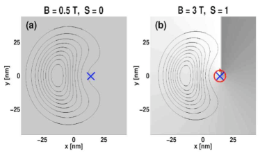
Figure 2: Reduced wave function of a two-electron quantum dot in (a) the singlet and (b) the triplet states. The fixed electron is marked by the cross to the right. The contours give the logarithmic electron density of the probing electron and the gray scale illustrates the phase of the wave function. The phase jumps from $0$ to $2\pi$ on the line where the scale changes from white to darkest gray. In the singlet state, the electrons have opposite spins and there is no vortex. In the triplet state, the electrons have same spin and a vortex (circle with an arrow in the direction of phase gradient) is attached on top of the fixed electron in accordance with the Pauli principle. Due to fermion antisymmetry the phase changes by $2\pi$ if the probe electron is moved around the fixed electron in this case. From Harju (2005).

In the case of larger particle numbers, interpretation of the reduced wave function requires a careful analysis, since nodes for different reference frames of fixed particles may not coincide Graham et al. (2003). However, localized nodes can be readily identified as vortices. These include off-particle vortices, which are associated with holes in the particle density. Also particle-vortex composites can be identified as nodes attached to the immediate vicinity of particles.

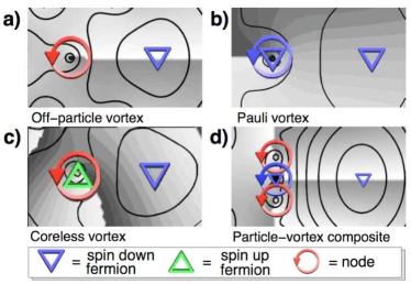
Figure 3: (Color online) Appearance of vortex structures in the reduced wave function. The figures show details of reduced wave functions for spin-$1/2$ fermions. The most probable position of the probing particle is to the right; the contours show the magnitude (on a logarithmic scale), and the gray-scale shows the phase (darkest gray = $0$, lightest gray = $2\pi$). a) An isolated, localized vortex which is not attached to any particle. b) A Pauli vortex (exchange hole) which is mandated by the wave function antisymmetry between interchange of indistinguishable fermions. c) A coreless vortex where the vortex core of spin-down component is filled by a spin-up fermion. d) A composite of a fermion (with a Pauli vortex) and two additional nodes which are bound to the particle, reminiscent of the Laughlin $\nu={1\over 3}$ state. From Saarikoski et al. (2009).

The reduced wave function as defined for single-component systems in Eq. (11) can be readily generalized also for multi-component systems with two or more particle species distinguishable from each other. The wave function is then a direct product of the wave functions of different particle species. As a consequence, the reduced wave function can still be written as in Eq. (11), although different particle species have to be distinguished. The reduced wave function depends on the species of the probe particle, unless the number of particles of each species is equal. The fact that phase singularities of one species coincide with particles of another species (see Fig. 3c) indicates formation of coreless vortices. This is discussed further in Sec. V. As an example, Figure 3 exemplifies the appearance of the reduced wave functions for different nodal structures, as here for fermions with spin-${1\over 2}$. Correlations in the many-body state can be further studied by analysing the reduced wave function in the vicinity of the most probable configuration(s).

II.4 Particle-hole duality in electron systems

In infinite quantum Hall liquids, particle-hole duality can be used to study vortex formation by interpreting holes as vortices Girvin (1996); Shahar et al. (1996); Burgess and Dolan (2001). Similar arguments for the symmetry of particle and hole states can be used in finite-size systems to gain insight into issues like vortex localization and fluctuations. We will here consider polarized electrons or, more generally, fermions of only one kind (i.e., spinless fermions). However, much of the considerations can be generalized to systems with more degrees of freedom, such as for example, spinor gases.

In the occupation number representation, the Hamiltonian for interacting electrons in the lowest Landau level can be written as

$$H_{p}=\sum_{i}\epsilon_{i}c_{i}^{\dagger}c_{i}+\sum_{ijkl}v_{ijkl}c_{i}^{\dagger}c_{j}^{\dagger}c_{l}c_{k}~{},$$ (12)

with annihilation and creation operators $c_{i}$ and $c_{i}^{\dagger}$ acting on determinants of states constructed from a given single-particle basis. Here we use the property that the occupation of each state for fermions can only be zero or one. We notice that the annihilation operator $c_{i}$ can be viewed as an operator creating a hole in the Fermi sea. Formally we can define new operators $d_{i}=c_{i}^{\dagger}$ and $d_{i}^{\dagger}=c_{i}$ as creation and annihilation operators of the holes. Equation (12) can then be written as a Hamiltonian of the holes. For the lowest Landau level, considering only states with good total angular momentum, it reduces to

$$H_{h}=\sum_{i}\tilde{\epsilon}_{i}d_{i}^{\dagger}d_{i}+\sum_{ijkl}v_{ijkl}d_{k}^{\dagger}d_{l}^{\dagger}d_{j}d_{i}+{\rm constant},$$ (13)

where

$$\tilde{\epsilon}_{i}=2\sum_{j}(v_{ijji}-v_{ijij})-\epsilon_{i}.$$ (14)

It is important to note that the interaction between the holes is equal to the interaction between the particles (assuming normal symmetry $v_{ijkl}=v_{klij}$), but the single-particle energies of the holes are affected by the interparticle interactions. We can thus solve the many-particle problem either for the particles, or for the holes. The use of the holes, however, does not reduce the complexity of the problem: The same accuracy of the solution requires diagonalization of a matrix which has the same size for particles or holes. However, considering holes instead of particles provides an alternative way to understand the localization of vortices in fermion systems Jeon et al. (2005); Manninen et al. (2005).

Using the above particle-hole duality picture we can treat the off-particle vortices as hole-like quasi-particles Kinaret et al. (1992); Ashoori (1996); Yang and MacDonald (2002); Saarikoski et al. (2004); Manninen et al. (2005). In electron systems, these vortices carry a charge deficiency of an elementary charge $e$. In the particle-hole duality picture the particles and holes (vortices) can be treated on equal footing. They form a quantum liquid of interacting electrons and vortices, where correlations play an important role.

For a correct description of the internal structure of the many-body system, we need to analyse all correlations between the constituents of the system, i.e., particle-particle, vortex-vortex, and particle-vortex correlations. The relative strength of these correlations determines the physics of the ground state. To give an example, clustering of electrons to a Wigner-crystal-like “molecule” of localized electrons is a signature of particularly strong particle-particle correlations. Analogously, the formation of a cluster or “molecule” of localized vortices shows the correlations between the vortex positions. Since the vortex dynamics is not independent of the electron dynamics, strong correlations between electrons and vortices may emerge, leading to the formation of particle-vortex composites.

II.5 Quantum Hall states

Vorticity increases with angular momentum, leading to the formation of particle-vortex composites at high magnetic fields. In the theory of the quantum Hall effect they were introduced to explain formation of incompressible electron liquids at fractional filling Laughlin (1983); Jain (1989). However, the phenomenon is more general, and similar in both fermion and boson systems where vorticity is sufficiently high Wilkin et al. (1998); Cooper and Wilkin (1999); Viefers (2008).

It should be noted that the analogy between quantum Hall states in finite-size droplets and corresponding states in the infinite 2D electron gas is only approximate, since the particle density inside the trapping potentials is often inhomogeneous, and edge effects play an important role. Nevertheless, in order to (at least approximatively) relate the states in finite size electron droplets to those in the infinite gas, the Landau level filling factor concept has been generalized to finite size systems. There is obviously no unique way to do such a generalization. However, a definition

$$\nu=\hbar{N(N-1)\over 2L},$$ (15)

which is based on the structure of Jastrow states, has been used in the $\nu<1$ regime Laughlin (1983); Girvin and Jach (1983). In large fermion systems, the filling factor becomes equal to the particle-to-vortex ratio, being a useful quantity also to classify rapidly rotating bosonic systems. Its relation to the fermion filling factor defined above is modified by the absence of Pauli vortices in the bosonic wave function.

The quantum Hall liquid is theoretically described by the Laughlin wave function Laughlin (1983) with its extensions, or by the related Jain construction Jain (1989); Jeon et al. (2004). These trial wave functions can be constructed just by using symmetry arguments without any detailed knowledge of the interparticle interactions. It has been shown that similar trial wave functions work for bosons and fermions Regnault and Jolicoeur (2003, 2004). Below we will discuss the vortex structures of these trial wave functions and demonstrate that one can map the boson wave function onto the fermion wave function, allowing a direct comparison of the vortex structures in these different systems.

II.5.1 Maximum density droplet state and its excitations

When an electron droplet is placed in a sufficiently strong magnetic field, it may polarize and the single-particle orbitals in the lowest Landau level become singly-occupied. (We remark that at some angular momenta, the electrons may polarize even if the Zeeman effect is ignored Reimann and Manninen (2002); Koskinen et al. (2007)). The spin-polarized compact droplet of electrons in the LLL, with total angular momentum $L=N(N-1)/2$, is called the maximum density droplet (MDD) state MacDonald et al. (1993). The MDD has the lowest possible angular momentum which is compatible with the Pauli principle. In the MDD, each electron carries a Pauli vortex and the wave function can be written as

$$\Psi_{\rm{MDD}}=\prod_{i<j}^{N}(z_{i}-z_{j})\exp\left[-\sum_{i=1}^{N}r_{i}^{2}/2\right]\ ,$$ (16)

where $z_{j}=x_{j}+iy_{j}$, $r^{2}=x^{2}+y^{2}$ and $x$ and $y$ are coordinates in the 2D plane. The MDD can be written as a single-determinantal wave function; for example, for seven particles it is $|11111110000\cdots\rangle$, where a “1” at position $i$ denotes an occupied state in the LLL with single-particle angular momentum $i-1$. Clearly, the MDD is the finite-size counterpart of the integer quantum Hall state with $\nu=1$.

Removing the Jastrow factor $\prod(z_{i}-z_{j})$ (i.e., the Pauli vortices) from the MDD in Eq. (16) leaves just a product of Gaussians which form the non-rotating bosonic ground state. The MDD state can therefore be interpreted as a fermionic “condensate”-like state of particles that engulf the flux quanta and, in effect, move in a zero magnetic field. In this way, the MDD state with $L_{\rm MDD}=N(N-1)/2$ is closely related to the non-rotating $L=0$ state of a bosonic system. We discuss this relation further in Sec. II.6, where we show conceptually, that by removing the Pauli vortices from each fermion, the wave function of a fermion system at $L$ is often a good approximation for a bosonic state with angular momentum $L^{\prime}=L-L_{\rm MDD}$.

The first excitation of the MDD in the LLL can be approximated as a single determinant where one of the single-particle states is excited to a higher angular momentum. This state can be understood in two different ways. It is definitely a center-of-mass excitation, since

$$|11\cdots 110100\cdots\rangle=\sum_{i=1}^{N}z_{i}|\mathrm{MDD}\rangle~{}.$$ (17)

On the other hand, this state is also a simple single-particle excitation where a hole enters the droplet from the surface. This hole is associated with a phase singularity in the reduced wave function.

To illustrate the nodal structure of a MDD, we show in Fig. 4 (a), with seven particles as an example, the reduced wave function for this state. Figure 4 (b) shows the reduced wave function of the four-particle state $|1010101000\rangle$ with three holes in the MDD, demonstrating that the holes localize on the sites of the “missing” electrons, each of them carrying a vortex that is characterized by zero density at the core, and the corresponding phase change.

Figure 4: (Color online) (a) Reduced wave function of a 7-particle MDD-state, (b) the MDD state with three holes, and (c), (d) MDD state with a center-of-mass excitation. The upper panels show the phase and the lower panels the magnitude of the reduced wave function. The bullets mark the fixed particle positions.

It is important to note that in the reduced wave function, only the positions of the particles are fixed, while the vortices are free to choose their optimal positions. This is illustrated in Fig. 4 (c) and (d) for a center of mass excitation: When one of the atoms (here fixed at the vertices of a hexagon) is moved to the center, the free vortex correspondingly moves from the center to the hexagon.

II.5.2 Laughlin wave function

The angular momentum of a quantum Hall state increases with the formation of additional vortices. When there are three times more vortices than electrons ($\nu=1/3$), fermion antisymmetry is preserved if two additional vortices (on top of Pauli vortices) are attached to each fermion. The corresponding wave function is the celebrated Laughlin state

$$\Psi_{\rm{m}}=\prod_{i<j}^{N}(z_{i}-z_{j})^{m}\exp\left[-\sum_{i=1}^{N}r_{i}^{2}/2\right]\ ,$$ (18)

where the antisymmetry of fermion wave functions requires that the exponent $m$ is an odd integer Laughlin (1983). The analogous wave function for a boson system in a trap is given by even values of $m$. The exponent $m$ is related to the filling factor, $\nu=1/m$, and to the angular momentum $L=mN(N-1)/2$. According to computational studies that apply diagonalization schemes to the many-body Hamiltonian (see Sec. III below), the Laughlin wave function with $\nu=1/3$ gives a good approximation of the ground state at the corresponding filling factors in finite-size quantum Hall droplets. We discuss this regime of strong correlations in the context of rapidly rotating quantum droplets in Sec. IV.6.

II.5.3 Jain construction and composite particles

The composite-fermion (CF) theory Jain (1989, 2007) generalizes the Laughlin wave function to a larger set of possible filling fractions. The basic idea is that when an even number of vortices, or flux quanta, is bound to electrons, these interact less as the vortices keep them apart, i.e., the exchange hole is widened by the cores of bound vortices. In addition, the composites move in an effective magnetic field that is weaker than the original one.

Formally, the composite fermion wave function can be written as Jain (2007)

$$\Psi_{\rm CF}={\cal P}_{\rm LLL}\psi_{\rm S}\prod_{i>j}(z_{i}-z_{j})^{m},$$ (19)

where $\psi_{\rm S}$ is a single Slater determinant of single-particle states, the product $\prod(z_{i}-z_{j})^{m}$ adds $m$ vortices at each electron and the operator ${\cal P}_{\rm LLL}$ projects the wave function to the lowest Landau level. If $\psi_{\rm S}$ is taken to be the MDD, Eq. (16) and Eq. (19) lead to the Laughlin wave function for the fractional Hall effect with filling factor $\nu=1/(m+1)$ and no projection to the LLL is needed. However, $\psi_{\rm S}$ is not restricted to the LLL, which allows constructing the states along the whole yrast line. For example, in order to get the MDD of composite particles, we have to take for $\psi_{\rm S}$ a MDD of states with negative angular momenta, which means replacing $z_{i}$ and $z_{j}$ with their complex conjugates $z_{i}^{*}$ and $z_{j}^{*}$ in Eq. (16). Note that the states with negative angular momenta are at higher Landau levels. Multiplying this by $\prod(z_{i}-z_{j})^{2}$ and projecting to the LLL gives the normal MDD wave function of Eq. (16). Wave functions between $\nu=1$ and $\nu=1/3$ can be obtained by starting from properly chosen Slater determinants for $\psi_{\rm S}$ Jain (2007). The projection to the LLL, however, is the most difficult part of the Jain construction. In practice, it can be done by replacing $z_{i}^{*}$’s by partial derivatives Girvin and Jach (1984).

The composite fermion picture accurately describes states at high angular momentum ($L\gg L_{\rm MDD}$) where two vortices (in addition to the Pauli vortex) are attached to each electron. However, for the states immediately above the MDD ($L\approx L_{\rm MDD}$) the CF theory still requires the attachment of two vortices to each electron. This means that the composite particle (electron and two vortices) has to move in an effective magnetic field which is opposite to the true magnetic field. In this case the projection operator ${\cal P}_{\rm LLL}$ will remove the two vortices (attached by the product $\prod(z_{i}-z_{j})^{2}$) and leads to the physically correct result that only one (Pauli) vortex is attached to each electron. The true number of vortices attached to each electron can thus be determined only after the projection to the lowest Landau level.

Comparison with exact numerical calculations have shown that the CF theory in the mean-field approximation does not predict all ground states correctly Harju et al. (1999); Yannouleas and Landman (2007). It is possible to go beyond mean-field theory, but the price to pay is that the beauty of not having variational parameters in the wave function is lost Jeon et al. (2007).

The CF theory has also been used for bosons Cooper and Wilkin (1999); Viefers et al. (2000); Cooper (2008); Viefers (2008). In this case an odd number of vortices are attached to each particle, i.e., the exponent $m$ in Eq. (19) is odd. Interestingly, the boson wave function is constructed as a product of two antisymmetric fermionic wave functions. The composite fermion picture naturally predicts a close relation between the bosonic and fermionic states along the yrast line, discussed in the next section.

II.6 Mapping between fermions and bosons

In the Laughlin state, the difference in angular momentum between the boson and fermion states equals that of the maximum density droplet, since trivially,

$$\prod_{i<j}^{N}(z_{i}-z_{j})^{m}=\prod_{i<j}^{N}(z_{i}-z_{j})\prod_{i<j}^{N}(z_{i}-z_{j})^{m-1}.$$ (20)

As long as the single-particle basis is restricted to the lowest Landau level, a similar transformation can be used to add a Pauli vortex to each bosonic particle, i.e., by multiplying the boson wave function with the determinant of the MDD,

$$\Psi_{\rm fermion}=\prod_{i<j}^{N}(z_{i}-z_{j})\Psi_{\rm boson}.$$ (21)

This transformation is valid, in addition to the Laughlin states, also for the Jain construction. It is expected that the same mapping is a good approximation for any many-particle state in the lowest Landau level Ruuska and Manninen (2005).

The accuracy of the boson-fermion mapping has been studied in detail by computing the overlaps between the exact fermion wave function, and the wave function obtained by transforming the exact boson state to a fermion state using Eq. (21) Borgh et al. (2008). At high angular momenta where the particles localize, the mapping becomes exact, while at small angular momenta the mapping is justified by the small number of possible configurations in the LLL. It is important to note that the free vortices of the bosonic system stay as free vortices also in the fermionic state. Only the Pauli vortices which localize at the particle positions are added. After transforming the bosons to fermions, particle-hole duality allows a detailed study of the vortex structure of the bosonic many-body wave function.

Figure 5 shows the calculated overlap between the transformed boson state and the exact fermion state as a function of the total angular momentum for eight particles. The transformation described by Eq. (21) does not always result in the ground state of the fermion system at given angular momentum. Instead, it may be one of the low-lying excitations and, consequently, the overlap drops to zero in these cases, as shown in Fig. 5. Moreover, the complexity of the wave function increases, while overlaps of the transformed wave function with the true fermion ground states tend to decrease with the number of particles $N$.

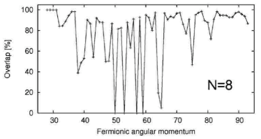
Figure 5: Overlap between the fermion ground state and the transformed boson ground state as a function of the total angular momentum, for eight particles. From Borgh et al. (2008).

Figure 6 illustrates the effect of the mapping for a droplet with $N=20$ particles in a harmonic trap at angular momenta where three free vortices form. The radial density profile of the bosonic state shows a minimum at the expected radial distance. When the bosonic state is transformed to a fermionic one, its radial density expands and becomes nearly identical to the exact density of the corresponding fermion system. The mapping allows to study the internal structure of the vortex lattice in the particle-hole duality picture: Figure 6 also shows the particle-particle and vortex-vortex correlation functions, indicating similar localization of three vortices in both cases.

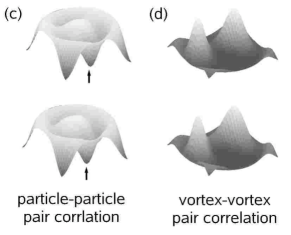
Figure 6: Mapping between boson and fermion states. The upper panels show the particle density of 20 bosons (a) and fermions (b) with Coulomb interactions, in the region of three vortices as a function of the radial distance of the droplet center. For bosons, the density of the mapped fermion system is shown as a dashed line. The lower panels show in coulmn (c) the particle-particle pair-correlations determined from the fermion wave functions. The position of the reference point is marked by the arrow at the bottom of the exchange-correlation hole. In column (d) the corresponding vortex-vortex pair-correlations are shown.

The simple mapping of Eq. (21) is computationally demanding when the particle number increases. This is due to the fact that every configuration of the boson wave function fragments to numerous fermion configurations. A simpler mapping was suggested by Toreblad et al. (2004) with a one-to-one correspondence between each boson and fermion configuration in the few-body limit. This mapping captures the most important configurations, but could not give as good overlaps.

The above transformation, Eq. (21), can be generalized to two-component quantum droplets. The transformation $L_{\rm boson}=L_{\rm fermion}-L_{\rm MDD}$ would attach a Pauli vortex to each boson. It is apparent that fermion states with $L_{\rm fermion}<L_{\rm MDD}$ cannot have bosonic counterparts in the LLL. Nevertheless, suggestive analogies in the (coreless) vortex structures between bosonic and fermionic states have been obtained in the few-particle limit Koskinen et al. (2007); Saarikoski et al. (2009).

III Computational many-body methods

The complexity of the many-body wave function grows exponentially with the particle number $N$, which makes computational studies indispensable. We here give a brief overview of the central methods used in the computational approaches to physics of rotation in both bosonic and fermionic systems, and their applicability to small droplets. As it is often the case for approximate approaches, the methods presented here have their limits of usability – no “universal” method exists which is superior to the others in capturing the essential physics in all parameter regimes.

The exact diagonalization or so-called configuration interaction (CI) method does not introduce any approximations to the solution of the Schrödinger equation apart from a cut-off in the used basis set. Therefore it is ideally suited to analyse correlations in the system. This method is, however, limited to relatively small particle numbers. Mean-field and density-functional methods are often needed to complement data for larger systems. In the density-functional approach, correlation effects are usually incorporated using local functionals of the spin densities. The method is able to reveal some of the underlying correlations in the system, but local approximations may fail to describe properly the complex particle-vortex correlations and formation of particle-vortex composites Saarikoski et al. (2005b). In the following, we draw upon the analogies between (a conventionally fermionic) density-functional theory and the Gross-Pitaevskii approach for bosons. We finally summarize the configuration interaction method for the direct numerical diagonalization of the many-body Hamiltonian.

Rather generally, the ground-state energy of an interacting many-body system trapped by an external potential $V_{\rm ext}({\bf r})$ can be written as a functional of the particle density $n({\bf r})$, summing up the kinetic, potential and interaction energy contributions,

$$E[n({\bf r})] = T_{0}[n({\bf r})]+\int\hbox{d}{\bf r}~{}n({\bf r})V_{\rm ext}({\bf r})+$$

$${1\over 2}\int\hbox{d}{\bf r}\int\hbox{d}{\bf r^{\prime}}~{}n({\bf r})n({\bf r^{\prime}})V^{(2)}({\bf r},{\bf r}^{\prime})+E_{\rm xc}~{},$$

where $T_{0}[n({\bf r})]$ is assumed to be the non-interacting kinetic energy functional, the second term accounts for the trap potential, the third term is the Hartree term for a two-particle potential $V^{(2)}$, and the exchange-correlation energy $E_{\rm xc}$ is defined to include all other many-body effects.

Introducing a set of single-particle orbitals $\psi_{i}({\bf r})$, the density may be expressed as

$$n({\bf r})=\sum_{i=0}^{\infty}f_{i}\mid\psi_{i}({\bf r})\mid^{2}~{},$$ (23)

with occupancies $\sum_{i}f_{i}=N$, following either bosonic or fermionic statistics. One can then write the non-interacting kinetic energy functional for the orbitals $\psi_{i}$ in the form

$$T_{0}[n({\bf r})]=\sum_{i}f_{i}\int\hbox{d}{\bf r}~{}\psi_{i}^{*}({\bf r})\left(-{\hbar^{2}\nabla^{2}\over 2m}\right)\psi_{i}({\bf r})~{}.$$ (24)

The crux of the matter is that Eq. (24) not necessarily holds for the exact kinetic energy functional $T[n({\bf r})]$. In many cases there will be a substantial correlation part in the kinetic energy functional that is not accounted for by the expressions above. In the spirit of density-functional theory Dreizler and Gross (1990), the last term in Eq. (III), $E_{\rm xc}$, thus has the task to collect what was neglected by this assumption, together with the effects of exchange and correlation that originate from the difference between the true interaction energy, and the simple Hartree term. It is important to note that the Hohenberg-Kohn theorem guarantees that this quantity is a functional of only the density, $E_{\rm xc}=E_{\rm xc}[n({\bf r})]$.

III.1 The Gross-Pitaevskii approach for trapped bosons

III.1.1 Gross-Pitaevskii equation for simple condensates

In the case of bosons, for a simple condensate all bosons are in the lowest state $\psi_{0}({\bf r})$ and the particle density is

$$n({\bf r})=|\psi_{0}({\bf r})|^{2}=N\mid\phi_{0}({\bf r})\mid^{2}$$ (25)

where the condensate wave function $\psi_{0}({\bf r})$ is normalized to $N$, and the corresponding “order parameter” $\phi_{0}({\bf r})$ to unity.

By using contact interactions and ignoring the correlations in Eq. (III) one obtains the well-known Gross-Pitaevskii energy functional,

$$E[n({\bf r})] = \int\hbox{d}{\bf r}\left[-{\hbar^{2}\over 2m}\mid\nabla\psi_{0}({\bf r})\mid^{2}\right.$$

$$\left.+V_{\rm ext}({\bf r})\mid\psi_{0}({\bf r})\mid^{2}+{1\over 2}g\mid\psi_{0}({\bf r})\mid^{4}\right]~{}.$$

Finding the ground state usually amounts to a variational procedure, i.e., independent variations of $\psi$ and $\psi^{*}$ under the condition that the total number of particles in the trap is constant. For the variation with respect to $\psi_{0}^{*}$,

$${\delta\over\delta\psi_{0}^{*}({\bf r})}\left[E[\psi_{0},\psi_{0}^{*}]-\mu\int\hbox{d}{\bf r}\mid\psi_{0}({\bf r})\mid^{2}\right]=0~{},$$ (27)

where the chemical potential $\mu$ plays the role of a Lagrange multiplier to fulfill the constraint. We then arrive at the time-independent Gross-Pitaevskii equation,

$$\left[-{\hbar^{2}\over 2m}\nabla^{2}+V_{\rm ext}({\bf r})+g\mid\psi_{0}({\bf r})\mid^{2}\right]\psi_{0}({\bf r})=\mu\psi_{0}({\bf r})~{}$$ (28)

having the typical form of a self-consistent mean-field equation. The corresponding $N$-particle bosonic wave function is

$$\psi({\bf r}_{1},{\bf r}_{2},...,{\bf r}_{N})=\prod_{i=1}^{N}\psi_{0}({\bf r}_{i})~{}.$$ (29)

The Gross-Pitaevskii approach, derived already in the 60’s independently by  Gross (1961) and Pitaevskii (1961), has been applied extensively for the theoretical description of inhomogeneous and dilute Bose gases at low temperatures. It is often convenient to solve the Gross-Pitaevskii equations in the imaginary-time evolution method, using a fourth-order split-step scheme Chin and Krotscheck (2005).

III.1.2 Gross-Pitaevskii approach for multi-component systems

The above Gross-Pitaevskii equation for a simple single-component Bose condensate Eq. (28) can be straightforwardly generalized also to multiple components of distinguishable species of particles. Let us consider as an example a two-component gas of atoms of kinds $A$ and $B$, that are interacting through the usual $s$-wave scattering with equal interaction strengths $g=g_{AA}=g_{BB}=g_{AB}$. The order parameters $\psi_{A}$ and $\psi_{B}$ of the two components then play an analogous role than the spin “up” and “down” orbitals in the spin-dependent Kohn-Sham formalism (see Sec. III.2). The corresponding Gross-Pitaevskii energy functional in the rest frame is simply

$$E=\sum_{\sigma=A,B}\int\mathrm{d}{\bf r}\psi_{\sigma}^{*}\biggl{(}-{\hbar^{2}\nabla^{2}\over 2M}+V_{\rm ext}({\bf r})\biggr{)}\psi_{\sigma}+$$

$${g\over 2}\int\mathrm{d}{\bf r}\bigl{(}\mid\psi_{A}\mid^{4}+\mid\psi_{B}\mid^{4}+2\mid\psi_{A}\mid^{2}\mid\psi_{B}\mid^{2}\bigr{)}~{}~{}$$ (30)

where $\sigma=\{A,B\}$ plays the role of a pseudospin $1/2$. In analogy to the single-component case described above, we minimize the energy functional with respect to $\psi_{A}^{*}$ and $\psi_{B}^{*}$, which results in two coupled Gross-Pitaevskii equations:

$$\biggl{(}\frac{{\bf p}^{2}}{2M}+{1\over 2}M\omega^{2}{\bf r}^{2}+g(|\psi_{A}|^{2}+|\psi_{B}|^{2})\biggr{)}\psi_{A} = \mu_{A}\psi_{A}$$

$$\biggl{(}\frac{{\bf p}^{2}}{2M}+{1\over 2}M\omega^{2}{\bf r}^{2}+g(|\psi_{B}|^{2}+|\psi_{A}|^{2})\biggr{)}\psi_{B} = \mu_{B}\psi_{B}~{}.~{}~{}$$

Naturally, it is required that $N_{A}=\int\mathrm{d}{\bf r}|\psi_{A}|^{2}$ and $N_{B}=\int\mathrm{d}{\bf r}|\psi_{B}|^{2}$, which determines the chemical potentials $\mu_{A}$ and $\mu_{B}$. One may choose to normalize the order parameter of one of the components, say B, to unity. Then, $N_{A}$ is determined by the ratio $N_{A}/N_{B}$. For the total angular momentum, $L=\int\mathrm{d}{\bf r}(\psi_{A}^{*}\hat{L}_{z}\psi_{A}+\psi_{B}^{*}\hat{L}_{z}\psi_{B})=L_{A}+L_{B}$. The above mentioned imaginary-time evolution method is also in the multi-component case the method of choice to numerically solve the Gross-Pitaevskii equations.

III.2 Density-functional approach

The density-functional theory for the solution of many-body problems in physics and chemistry was proposed by Hohenberg, Kohn and Sham in the 1960’s Hohenberg and Kohn (1964); Kohn and Sham (1965). It is a correlated many-body theory where all the ground-state properties can in principle be calculated from the particle density Hohenberg and Kohn (1964); Kohn (1999); Dreizler and Gross (1990); Parr and Yang (1989). The original density-functional theory did not take into account the effects of a non-zero spin polarization and currents induced by an external magnetic field. Since these effects have marked consequences on the ground-state properties of the rotating many-body systems, for a description of quantum dots in strong magnetic fields, extensions such as the spin-density-functional method Gunnarsson and Lundqvist (1976); von Barth (1979) and the current-spin-density-functional method Vignale and Rasolt (1987, 1988); Rasolt and Perrot (1992); Capelle and Gross (1997) were applied. For a very pedagogic review on density-functional theory, we refer to Capelle (2006).

III.2.1 Spin-density-functional theory for electrons

In the spin-density-functional formalism one can derive self-consistent Kohn-Sham equations for the Hamiltonian Eq. (6) that describes $N$ interacting electrons in an external magnetic field:

$$\nabla^{2}V_{\rm H}=-{n/\epsilon}$$ (31)

$$n_{\sigma}({\bf r})=\sum^{N_{\sigma}}_{i}|\psi_{i,\sigma}({\bf r})|^{2}$$ (32)

$$\left\{{1\over 2m^{*}}\left[{\bf p}+{e}{\bf A}({\bf r})\right]^{2}+V_{\rm eff,\sigma}({\bf r})\right\}\psi_{i,\sigma}=\epsilon_{i,\sigma}\psi_{i,\sigma}~{}.$$ (33)

Eq. (31) is the Poisson equation for the solution of the Hartree potential $V_{\rm H}$, i.e. the Coulomb potential for the electronic charge density $n$, where $\epsilon$ is the dielectric constant of the medium. Eq. (32) determines the spin densities, where $\sigma=\{\uparrow,\downarrow\}$ is the spin index, $N_{\sigma}$ is the number of electrons with spin $\sigma$, the $\psi_{i,\sigma}$’s are the one-particle wave functions, and the summation is over the $N_{\sigma}$ lowest states (which here have fermionic occupancy). In Eq. (33), the effective scalar potential for electrons

$$V_{\rm eff,\sigma}({\bf r})=V_{\rm ext}({\bf r})+V_{\rm H}({\bf r})+V_{\rm xc,\sigma}({\bf r})+V_{\rm Z}$$ (34)

consists of the external scalar potential $V_{\rm ext}$, the Hartree potential $V_{\rm H}$, the exchange-correlation potential $V_{\rm xc}$ and the Zeeman term $V_{Z}=g^{*}\mu_{B}Bs_{\sigma}$, where $\mu_{B}$ is the Bohr magneton, $s_{\sigma}=\pm 1/2$, $B$ is the magnetic field and $g^{*}$ is the gyromagnetic ratio. All the interaction effects beyond the Hartee potential $V_{\rm H}$ are incorporated in the exchange-correlation potential $V_{\rm xc}$. A more fundamental generalization of the density-functional method for systems in external magnetic fields is the current-density-functional method Vignale and Rasolt (1987, 1988), where the vector potential A is replaced by an effective vector potential $\hbox{\bf A}_{\hbox{eff}}=\hbox{\bf A}+\hbox{\bf A}_{\hbox{xc}}$ accounting for many-particle effects on the current densities. In the above equations, only the conduction electrons of the semiconductor are explicitly included in the theory, while effects of the lattice are incorporated via material parameters such as effective mass, dielectric constant and effective $g$-factor.

Density-functional approaches are often combined with local approximations for the exchange-correlation potential where $V_{\rm xc}$ in actual calculations is usually taken as the exchange-correlation potential of the uniform electron gas. In 2D electron systems, approximate parametrizations have been calculated Tanatar and Ceperley (1989); Attaccalite et al. (2002) and the approach leads to a set of mean-field-type equations. It should be emphasized that density-functional theory a priori is not a mean-field method but a true many-particle theory. Its strength is that it very often may provide accurate approximations to the ground state properties such as the total energy with the computational effort of a mean-field method. It is important to note that single-particle states (Kohn-Sham orbitals) and their eigenenergies are auxiliary parameters in the Kohn-Sham equations. However, as an approximation, the Kohn-Sham orbitals may still be used to construct a single Slater determinant to account for the nodal structure.

The density-functional approach in the local density approximation, as well as the unrestricted Hartree-Fock method, may show broken symmetries in particle and current densities. This is often interpreted as reflections of the internal structure of the exact many-body wave function. However, a caveat is that implications of symmetry-breaking patterns may in some cases yield wrong implications of the actual many-body structure of the exact wave function. This problem is well-known in quantum chemistry as “spin contamination”, and we refer to Szabo and Ostlund (1996) as well as the more recent articles by Schmidt et al. (2008), as well as Harju et al. (2004) and Borgh et al. (2005) for a thorough discussion. This conceptual problem of spin-density-functional theory often calls for an analysis by more exact computational methods.

III.2.2 Density-functional theory for bosons

The Gross-Pitaevskii mean-field approach discussed above certainly is the most widely used theoretical tool to describe Bose-Einstein condensates, and has been extensively applied to investigate vortex structures in rotating systems. Clearly, it is a density-functional method based on the functional Eq. (III.1.1) where the density is a square of a single one-particle state, Eq. (25). However, there are many situations where correlations determine the many-body states, that cannot be captured by the standard Gross-Pitaevskii approach Bloch et al. (2008).

On the other hand, the exact diagonalization method, which captures all correlation effects, cannot be used for systems which consist of more than just a few particles. A bosonic density-functional theory has been introduced as one possible way to go beyond the mean-field approximation Hunter (2004); Braaten and Nieto (1997); Kim and Zubarev (2003); Griffin (1995); Nunes (1999); Rajagopal (2007); Capelle (2008). For ground states this approach is not very efficient due to a lack of nodal structure in the wave function. This, however, is different in the case of fragmented or depleted condensates Mueller et al. (2006); Capelle (2008).

Following the well-known Hohenberg-Kohn theorem, the energy functional $E[n({\bf r})]$ is minimized by the ground-state density. This in fact is independent of whether the particles are bosons or fermions, and a corresponding density-functional approach to bosonic systems was more recently formulated by Capelle (2008). Taking the $E_{\rm xc}$ contributions into account, the variation of Eq. (III) adds the potential Nunes (1999)

$$V_{\rm xc}={1\over\psi({\bf r})}{\delta E_{\rm xc}\over\delta\psi({\bf r})}~{}.$$ (35)

However, $\psi({\bf r})$ cannot describe correctly the many-body state, if the ground state contains “uncondensed” bosons, or requires a macroscopic occupation of more than one single-particle state. Capelle (2008) showed that since the Hohenberg-Kohn theorem still holds in these cases, the Gross-Pitaevskii equation, Eq. (28), can be more generally expressed as

$$\left[-{\hbar^{2}\over 2m}\nabla^{2}\right. + V_{\rm ext}({\bf r})+\int\hbox{d}{\bf r}~{}n({\bf r})n({\bf r}^{\prime})V^{(2)}({\bf r}-{\bf r}^{\prime})$$ (36)

$$+ \left.{\delta E_{\rm xc}[n]\over\delta n({\bf r})}\right]\psi_{i}({\bf r})=\epsilon_{i}({\bf r})\psi_{i}({\bf r})~{},$$

with the label $i$ now running over all solutions of the equation. The orbitals $\psi_{i}$ do not have a simple relation to the Gross-Pitaevskii order parameter, but they do provide the correct density via Eq. (23) with (bosonic) occupancies $f_{i}$ of the states $\psi_{i}$ . These equations took a form that is indeed very familiar from the usual Kohn-Sham equations for fermions discussed above  Capelle (2008). For an account of viable approximations to $E_{\rm xc}$, we refer to Capelle (2008), as well as  Nunes (1999) and  Kim and Zubarev (2003).

III.3 Exact diagonalization method

The configuration interaction (CI) method, also called “exact diagonalization”, is a systematic scheme to expand the many-particle wave function. It traces back to the early days of quantum mechanics, to the work of Hylleraas (1928) on the Helium atom. It has been extensively used in quantum chemistry, but nowadays found its use also for quantum nanostructures as well as cold atom systems. In the basic formulation of this approach, one takes the eigenstates of the non-interacting many-body problem (called configuration) as a basis and evaluates the interaction matrix elements between these states. The resulting Hamiltonian matrix is then diagonalized.

Rules to calculate the matrix elements were originally derived by Slater (1929, 1931) and Condon (1930), and developed further by Löwdin (1955). We note that the use of the term “exact diagonalization” that has been widely adopted by the community, often replacing the quantum-chemistry terminology of “configuration interaction”, might in some cases be misleading, as truly exact results are obtained only in the limit of an infinite basis.

Consider a Hamiltonian split into two parts $\mathcal{H}=\mathcal{H}_{0}+\mathcal{H}_{I}$, where the Schrödinger equation of the first part is solvable,

$$\mathcal{H}_{0}|\phi_{i}\rangle=\varepsilon_{i}|\phi_{i}\rangle~{},$$ (37)

and the states $|\phi_{i}\rangle$ form an orthonormal basis. The solution for the full Schrödinger equation can be expanded in this basis as $|\psi\rangle=\sum_{i}\alpha_{i}|\phi_{i}\rangle$. Inserting this into the Schrödinger equation

$$\mathcal{H}|\psi\rangle=E|\psi\rangle$$ (38)

results in

$$(\mathcal{H}_{0}+\mathcal{H}_{I})\sum_{i}\alpha_{i}|\phi_{i}\rangle=E\sum_{i}\alpha_{i}|\phi_{i}\rangle\ ,$$ (39)

or a matrix equation

$$(H_{0}+H_{I})\mbox{\boldmath$\alpha$}=E\mbox{\boldmath$\alpha$}\ ,$$ (40)

where $H_{0}$ is a diagonal matrix with $\langle\phi_{i}\mid H_{0}\mid\phi_{i}\rangle=\varepsilon_{i}$ and the elements of $H_{I}$ are $\langle\phi_{j}|\mathcal{H}_{I}|\phi_{i}\rangle$. The vector $\alpha$ contains the values $\alpha_{i}$. In principle, the basis $\{|\phi_{i}\rangle\}$ is infinite, but the actual numerical calculations must be done in a finite basis. The main computational task is to calculate the matrix elements of $H_{I}$ and to diagonalize the corresponding matrix. The convergence as a function of the size of the basis set depends on the problem at hand, and is of course fastest for the cases where $\mathcal{H}_{I}$ is only a small perturbation to $\mathcal{H}_{0}$.

The basic procedure is straightforward text-book knowledge of quantum mechanics. However, one should bear in mind that much of the state-of-the-art computational knowledge must be employed when it comes to numerical implementations, in order to model large and highly-correlated systems.

The usual starting point for the exact diagonalization method is the non-interacting problem. In 2D harmonic potentials, harmonic oscillator states - or Fock-Darwin states of non-interacting particles in a magnetic field - can be used to construct a suitable basis, but it can also be optimized by using states from, e.g., Hartree-Fock or density-functional methods (for a recent example, see the work by Emperador et al. (2005)). For fermions, the solution is a Slater determinant formed from the eigenstates of the single-particle Hamiltonian. The corresponding symmetric $N$-boson state is a permanent. In the non-interacting ground state, all the bosons occupy the same state. On the other hand, fermions occupy the $N$ lowest states due to the Pauli principle. Due to interactions, other configurations than the one of the non-interacting ground state have a finite weight in the expansion of the many-particle wave function. Often, the increasing complexity of the quantum states with large interaction strengths and large system sizes causes severe convergence problems, where the number of basis states needed for an accurate description of the many-body system increases far beyond computational reach.

In rotating weakly-interacting systems confined by harmonic potentials, a natural restriction of the single-particle basis is the LLL. It provides a well-defined truncation of the Hilbert space for the given value of the angular momentum $L$ and particle number $N$. The LLL approximation in the harmonic confinement implies that the diagonal part of the Hamiltonian is independent of the configuration, and solving the Hamiltonian reduces to the diagonalization of the potential energy of the interparticle interactions. This truncation eliminates also the usual issue of regularization that emerges with the use of contact forces in exact diagonalization schemes, see for example,  Huang (1963): The direct diagonalization of the Hamiltonian with contact interactions on a complete space yields unphysical solutions unless the class of allowed basis functions obeys special and often impractical boundary conditions Esry and Greene (1999). The Hamiltonian matrix in the LLL is often sparse, and in the limit of large $N$ and $L$ it is usually diagonalized in a Lanczos scheme Lehoucq et al. (1997).

IV Single-component quantum droplets

In the following, we describe the structure of single-vortex states and the formation of vortex “clusters” or vortex “molecules”, as they are also often called, in single-component systems. In the strongly-correlated regime of rapid rotation, the increased vortex density leads to finite-size counterparts of fractional quantum Hall states, both with bosons and fermions. The existence of giant or multiple-quantized vortices in anharmonic traps is also discussed.

IV.1 Vortex formation at moderate angular momenta

IV.1.1 Vortex formation in trapped bosonic systems

Following the achievement of Bose-Einstein condensation in trapped cold atom gases, experimental setups were devised to study their rotational behavior. The first observation of vortex patterns in these systems was made for a two-component Bose condensate consisting of two internal spin states of ⁸⁷Rb, where the formation of a single vortex was detected Matthews et al. (1999). Soon after this seminal experiment, evidence for the occurrence of vortices was found by literally “stirring” a one-component gaseous condensate of rubidium by a laser beam  Madison et al. (2000). While the vortex cores are too small to be directly observed optically (the core radius is typically from 200 to 400 nm), vortex imaging is possible if the atomic cloud first is allowed to expand by turning off the trap potential Madison et al. (2000). In this way, regular patterns of vortices were observed in the transverse absorption images of the rubidium condensate (see Fig. 7). At moderate rotation, above a certain critical frequency $\Omega_{c}$, first a central “hole” occurred, clearly identified as a pronounced minimum in the cross-section of the density distribution, shown to the right in Fig. 7b).

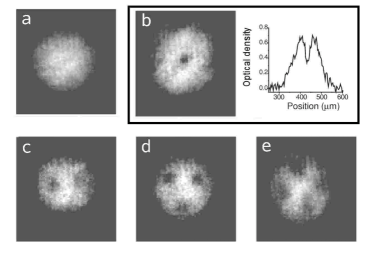
Figure 7: Transverse absorption images of a Bose-Einstein condensate of ⁸⁷Rb, stirred with a laser beam. As the rotation of the trap increases from a) to e), a clear vortex pattern evolves. The inset to the right of panel b) shows the cross section of the optical density which shows a pronounced minimum at the center. After  Madison et al. (2000).

As the rotation of the trap increases, a 2nd, 3rd and 4th vortex penetrates the bosonic cloud. The vortices then arrange in regular geometric patterns. Intriguingly, these patterns coincide with the geometries of Wigner crystals of repulsive particles, as they have been found for example in quantum dots at low electron densities, or strong magnetic fields Reimann and Manninen (2002). Vortices with the same sign of the vorticity effectively repel each other (see for example, Castin and Dum (1999)). This supports the view of Wigner-crystal-like arrangement of vortices, throwing an interesting light on the much debated melting of the vortex lattice at extreme rotation (see also Sec. IV.4 below). The interplay between vortex- and particle localization in a rotating harmonic trap is further discussed in Section IV.2 below.

The theory of vortices in rotating BEC’s has attracted a lot of attention in the recent years, and much work has been published for the Thomas-Fermi regime of strong interactions, see for example, Rokhsar (1997); García-Ripoll and Pérez-García (1999); Feder et al. (1999a, b); Svidzinsky and Fetter (2000). In this limit, which applies to most experiments on rotating BEC’s, the coherence length $\xi=(8\pi na)^{1/2}$, where $n$ is the density and $a$ the scattering length, is much smaller than the extension of the bosonic cloud, and some properties of the system resemble those of a bulk superfluid Baym and Pethick (1996). In the case of weakly interacting bosons in a harmonic trap, however, the coherence length becomes larger than the size of the cloud, and the interaction energy plays the dominant role: the mesoscopic limit is reached, where the system becomes like a quantum-mechanical Knudsen gas Mottelson (2001). In this mesoscopic limit, the analogies between trapped bosons and quantum dots at strong magnetic fields become apparent. This regime of weak interactions is our primary concern in the following.

IV.1.2 Weakly interacting bosons under rotation

Let us now consider a dilute system of $N$ spinless bosons in a harmonic trap, weakly interacting by the usual contact force $g\delta({\bf r}-{\bf r}_{0})$, where $g=4\pi\hbar^{2}a/M$ is the strength of the effective two-body interaction with scattering length $a$ and atom mass $M$. The condition for weak interactions is that the interaction energy is much smaller than the quantum energy of the confining potential, i.e.,

$$ng\ll\hbar\omega\;,$$ (41)

where $n$ is the particle density. As explained in Sec. II.1.1 above, requiring maximum alignment of the total angular momentum, the relevant single-particle states of the oscillator are those of the LLL. This approach, which has earlier proven very successful for the description of the fractional quantum Hall regime for the electron gas, has been introduced for bosonic systems by Wilkin et al. (1998).

As mentioned in  II.1.1, the large degeneracy originating from the many different ways to distribute the $N$ bosons on the single-particle states of the LLL, is lifted by the interactions.

Identifying the elementary modes of excitation, Mottelson (1999) showed that besides the usual condensation into the lowest state of the oscillator, the yrast states (i.e. the states maximizing $L$ at a given energy, see Sec. II.1.1) involve additional kinds of condensations that are associated with the many different possibilities for distributing the angular momentum on the degenerate set of basis states in the LLL. For $1\ll L\ll N$, the yrast states and low-energy excitations as a function of $L$ can be constructed by a collective operator

$$Q_{\lambda}={1\over\sqrt{2N\lambda!}}\sum_{p=1}^{N}z_{p}^{\lambda}~{},$$ (42)

with coordinates of the $p$th particle $z_{p}=x_{p}+iy_{p}$.

In the case of attractive interactions, the lowest-energy state for fixed angular momentum is the one involving excitations of the center-of-mass of the cloud. The yrast state is then described by $\mid\Psi_{L}\rangle\sim(Q_{1})^{L}\mid\Psi_{L=0}\rangle$  Wilkin et al. (1998); Mottelson (1999).

In the case of repulsive interactions, for bosons in the LLL at $L=0$ the only possible state is the pure condensate in the $m=0$ single-particle orbital, thus maximizing the interaction energy. Increasing the angular momentum by one is possible via a center-of-mass excitation of the non-rotating state. For $L>1$ and $L\ll N$, the excitation energies of the modes $Q_{\lambda\neq 1}$ show that the yrast states are predominantly obtained by a condensation into the quadrupole ($\lambda=2$) and octupole ($\lambda=3$) modes, as shown by Mottelson (1999).

Bertsch and Papenbrock (1999) compared these results to a numerical computation of the yrast line. For the harmonic trap in the lowest Landau level, the problem can be solved straightforwardly by numerical diagonalization of the Hamiltonian Eq. (3). (See the discussion in Sec. III.3 above).

The resulting yrast line decreases with increasing $L$ for repulsive interactions, since centrifugal forces tend to keep the particles further apart when rotation increases (see Fig. 8 for the example of $N=25$ and $N=50$ bosons). It shows a linear decrease in energy with $L$, that extends up to $L=N$. This linearity was also found in a study within the Gross-Pitaevskii approach by Kavoulakis et al. (2000) (see below). The inset to Fig. 8 shows the excitation spectra for $N=50$ bosons at angular momenta $L\leq 18$. “Spurious” eigenstates occur that originate from a $SO(2,1)$ symmetry  Pitaevskii and Rosch (1998) only exciting the center-of-mass, i.e., the yrast spectrum at $L+1$ includes the full set of states at angular momentum $L$. (These center-of-mass excitations were excluded in the spectra shown in Fig. 8.) In a harmonic confinement the center-of-mass excitations are exactly separated from the internal excitations and they are known to exist also in Fermi systems Trugman and Kivelson (1985); Reimann and Manninen (2002).

The lower panel in Fig. 8 shows the occupancies of the lowest single-particle states for a $N=50$ bosonic state with angular momentum up to $L=N$. In agreement with the aforementioned results of  Mottelson (1999), at small $L/N$ the yrast states are mainly built from single-particle states with $m=0$, $m=2$ and $m=3$, respectively, where $m$ is the angular momentum of the single-particle state Bertsch and Papenbrock (1999).

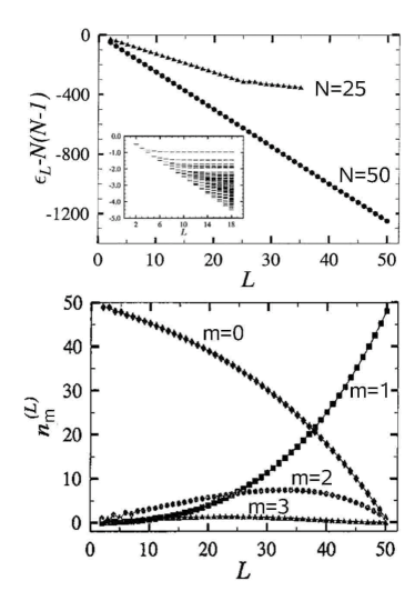
Figure 8: Upper panel: Many-body yrast lines for $N=25$ and $N=50$ spinless bosons in a harmonic confinement for angular momenta $2\leq L\leq 50$. The inset shows the excitation spectrum for $N=50$ and $L\leq 18$, excluding the spurious center-of-mass excitations, see text. From Papenbrock and Bertsch (2001). Lower panel: Occupancies of the lowest single-particle states of the harmonic oscillator in the lowest Landau level, for $m=0$ (diamonds), $m=1$ (squares), $m=2$ (circles) and $m=3$ (triangles). From  Bertsch and Papenbrock (1999). Calculations are within the lowest Landau level.

Approaching $L/N=1$, the yrast state takes a much simpler structure, with a dominant occupancy of the $m=1$ single-particle orbital. At $L/N=1$, a single vortex locates at the center of the cloud.

An analytic expression for the exact energies for $2\leq N\leq N$ was conjectured by Bertsch and Papenbrock (1999) and subsequently derived by Jackson and Kavoulakis (2000); in atomic units it reads

$$\epsilon_{L}={1\over 2}N(2N-L-2)~{}.$$ (43)

Smith and Wilkin (2000) derived analytically the exact eigenstate as an elementary symmetric polynomial of coordinates relative to the center-of-mass. Later, exact yrast energies for a universality class of interactions were derived Hussein and Vorov (2002); Vorov et al. (2003). Generalizing a conjecture by Wilkin et al. (1998) for the structure of the unit vortex at $L=N$,

$$\mid L=N\rangle=\Pi_{p=1}^{N}(z_{p}-z_{c})\mid 0\rangle$$ (44)

where $z_{c}=(z_{1}+z_{2}+\cdots+z_{N})/N$ is the center-of-mass coordinate,  Bertsch and Papenbrock (1999) could demonstrate that the exact wave function in the whole region $2\leq L\leq N$ is given by

$$\mid L\rangle = {\cal N}\sum_{p_{1}<p_{2}<...<p_{L}}(z_{p_{1}}-z_{c})$$ (45)

$$\times(z_{p_{2}}-z_{c})...(z_{p_{L}}-z_{c})\mid 0\rangle,$$

where ${\cal N}$ is a normalization constant, and the indices run over all particle coordinates, up to the total particle number $N$.

Let us now investigate the evolution of the pair-correlated densities, defined in section  II.3.3 above. Fig. 9 shows their contours, for $N=40$ bosons with the reference point located at a distance $r_{A}=3\ell_{0}$ (chosen outside the bosonic cloud for clarity; $\ell_{0}$ is the oscillator length). Starting from a homogeneous Gaussian density distribution at $L=0$, as $L/N$ increases, clearly the first vortex enters the cloud from its outer parts. At $L=N$, the (azimuthally symmetric) particle density has developed a pronounced central hole, that is also apparent from the correlation function shown in the lower right panel of Fig. 9. The nodal pattern of this state, as probed by conditional wave functions, clearly confirms the simple structure of the unit vortex (see e.g. the $L=N=5$ state in Fig. 31).

Figure 9: Equidensity lines of the pair-correlation function $P({\bf r},{\bf r}_{A})$ for $N=40$ spinless bosons at $L=28,32,36$ and $40$. For clarity, the reference point was located outside the cloud at ${\bf r}_{A}=(3,0)$. The vortex, which approaches the center from the right with increasing $L$, gives rise to a pronounced minimum in the pair-correlation plots. From  Kavoulakis et al. (2002).

For a discussion of the low-energy excitations at and around the unit vortex, we refer to Ueda and Nakajima (2006).

Recently, Dagnino et al. (2009b, a) studied the vortex nucleation process by calculating the density matrix obtained from the CI eigenstates for a trap with a small quadrupole deformation. A related early study was presented by Linn et al. (2001), who applied a variational method to investigate the ground state phase diagram in an axially asymmetric BEC. The analysis by  Dagnino et al. (2009b, a) indicated that when the rotation frequency of the axially deformed trap is increased and the system passes through the first vortex transition, two of the “natural orbitals” of the density matrix have equal weight. Nunnenkamp et al. (2009) also studied the noise correlations at criticality for the elliptic trap, while Parke et al. (2008) relate the transition to vortex tunneling in the process of nucleation.

In the light of the above-mentioned findings, however, it is worth noting that the overall picture strongly depends on the symmetry of the chosen trap deformation, and is further complicated by finite-size effects – the latter being an inevitable restriction in the CI method that becomes more severe, when the angular momentum no longer commutes with the Hamiltonian.

Figure 10: Vortex entry for a spherical bosonic cloud at angular momenta $l=L/N$. Shown are the surfaces of constant density obtained by the Gross-Pitaevskii method. The cloud flattens with increasing angular momentum. From  Butts and Rokhsar (1999).

In the Gross-Pitaevskii approach, the vortices are directly visible in the density as well as the phase of the order parameter, which breaks the rotational symmetry. Butts and Rokhsar (1999) and Kavoulakis et al. (2000) were among the first to apply this method to a weakly interacting, dilute condensate of bosonic atoms in a rotating harmonic trap. Fig. 10 shows the equidensity surfaces for the Gross-Pitaevskii order parameter $\Psi({\bf r})$ for the states along the yrast line between $L=0$ and $L=N$ Butts and Rokhsar (1999), demonstrating how the first vortex enters the cloud. In the non-rotating case, the condensate forms a lump with zero angular momentum at the center of the trap. Beyond a certain critical rotation, however, the ground state becomes a vortex state with one single-quantized vortex that manifests itself as a central hole in the density (see $l=1.0$ in Fig. 10). The phase of the order parameter changes by $2\pi$ when encircling this hole (see Fig. 15, upper panel, left). The value of the critical rotation frequency depends on the system parameters, but the angular momentum per particle $l=L/N$ equals unity when the vortex reaches the center. This result is also confirmed by the exact diagonalization calculations in the few-particle regime (see Fig. 12a). The same mechanism of vortex entry was also found in the Gross-Pitaevskii study by Kavoulakis et al. (2000). In the limit of large $N$, Jackson et al. (2001) compared the energies obtained in the Gross-Pitaevskii approach to those obtained by the CI method, and found that the mean-field results provide the correct leading-order approximation to the exact energies within the same subspace. For a more complete discussion of the mean-field theory of single-vortex formation in bosonic condensates, we refer to Fetter (2009).

IV.1.3 Single-vortex states in electron droplets

Two-dimensional electron droplets in quantum dots can be rotated by applying a perpendicular magnetic field. The number of confined electrons, as well as the rotation frequency can be controlled by an external gate voltage and the field strength, respectively.

In symmetric quantum dot devices the confining potential can often be modeled accurately by a 2D harmonic potential Matagne et al. (2002); Bruce and Maksym (2000); Nishi et al. (2006). These systems would therefore be ideal testbeds for analysis of vorticity in rotating fermionic systems with repulsive interactions. However, direct experimental detection of signatures of vortex formation in the electron density is very difficult due to small charge densities inside the electron droplet, that is often buried in a semiconductor heterostructure. Attempts to extract any signatures of vortex formation have usually focused on the analysis of quantum transport measurements Saarikoski and Harju (2005); Güçlü et al. (2005).

In weak magnetic fields, electron droplets in quantum dots are composed of electrons which have their spin either parallel or antiparallel to the magnetic field. As the strength of the magnetic field increases, the system gradually spin-polarizes. For details on this process and electronic structure of quantum dots in this regime we refer to the reviews by Kouwenhoven et al. (2001) and Reimann and Manninen (2002). The first totally spin-polarized state in the LLL is the maximum density droplet (MDD) state MacDonald et al. (1993) discussed in Sec. II.5.1. The existence of this state was firmly established experimentally Oosterkamp et al. (1999) using quantum transport measurements. When the angular momentum is further increased with the magnetic field, the MDD state reconstructs, and a vortex may form inside the electron droplet.

The breakdown mechanism of the MDD and its interpretation has been one of the most discussed subjects in the early theoretical studies of quantum dots. Many of these works were inspired by the theory of excitations of the quantum Hall states. MacDonald et al. (1993) as well as Chamon and Wen (1994) discussed the possibility of edge excitations in large quantum Hall systems. Their studies suggested that the MDD would break up via reconstruction of the MDD edge. This possibility was examined further by Goldmann and Renn (1999) using a set of trial wave functions which described a MDD state surrounded by a ring of localized electrons. In large quantum dots, density-functional studies indicated a charge-density wave (CDW) solution along the edge of the dot Reimann et al. (1999) around a rigid MDD-like dot center. These studies showed that for larger dot sizes, a rotating single-component fermion liquid would not develop vortex states but instead the edge of the system would be excited around a rigid MDD-like center. However, Hartree-Fock calculations for small electron droplets predicted that holes are created inside the droplet that would bunch to minimize the exchange energy Ashoori (1996). Yang and MacDonald (2002) used the exact diagonalization approach and also found the MDD state unstable towards creation of internal holes in high magnetic fields. A skyrmion type of excitation above the MDD state was considered by Oaknin et al. (1996). This study generalized the theory of skyrmion type of excitations in the 2D electron gas (2DEG) Ezawa (2000) to finite-size quantum Hall droplets, which was motivated by localization of skyrmions in a Zeeman field. They proposed a wave function whose form for large particle numbers is that of a mean-field type of skyrmion excitation. Heinonen et al. (1999) found also edge spin textures in an ensemble density-functional approach. A skyrmion-type spin texture can be treated as another manifestation of vorticity, as pointed out in the context of two-component bosonic condensates, see Sec. V. For quantum dots with four and six electrons, a recent study within the CI method showed that meron excitations are dominant for the lowest-lying states in very small quantum dots at strong magnetic fields (in the limit of vanishing Zeeman coupling), see Petkovic and Milovanovic (2007).

Holes in the charge density were identified as vortex cores in the density-functional studies of quantum dots Saarikoski et al. (2004) (see Fig. 11). This work also directly showed with the configuration interaction method that for the $N=6$ case the nodal structure of the many-body wave function revealed an isolated vortex at the center of the dot.

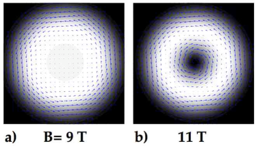
Figure 11: a) Charge density (gray scale) and current density (arrows) in the maximum density droplet state of a 6-electron droplet at magnetic field $B=9\;{\rm T}$ calculated with the density-functional method. The angular momentum is $L=15$, and the density inside the droplet is uniform. The solution shows also an edge current reminiscent of those in quantum Hall states. b) The single-vortex state in the same droplet at slightly increased magnetic field of $B=11~{}T$ with $L=21$. It shows a pronounced vortex hole in the middle with a rotating current around it. Adapted from the results of Saarikoski et al. (2004).

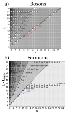
Figure 12: Systematics of boson and fermion ground states. When the external rotation $\Omega$ is gradually increased from zero, a droplet of $N$ particles goes through a series of ground states with increasing angular momentum $L$. Stars mark these $L$ values as a function of $N$ for a) boson droplets and b) fermion droplets. Calculations are done with the exact diagonalization method in the lowest Landau level approximation, and a harmonic confining potential Eq. (4). In the fermion results in b), the angular momentum of the maximum density droplet, $L_{\rm MDD}$, is substracted from $L$. The linear $N$ dependence of the first $(N,L)$-combination in bosonic systems (red arrow) indicates that the first $L$ above the non-rotating state has a central vortex. Fermionic systems with repulsive interactions show a similar behaviour only until $N=12$, where the breakdown mechanism of the MDD clearly changes (blue arrow), and a non-localized node emerges at a finite distance from the center. After Harju (2005) and Suorsa (2006).

These results suggested that the first magnetic flux quantum, which penetrates the electron droplet, is a free vortex and not bound to any particle as in the Laughlin wave function. Configuration interaction calculations for few-electron quantum dots provided further evidence for vortex formation in few-electron systems Toreblad et al. (2004); Tavernier et al. (2004); Manninen et al. (2005). In the few-electron regime, the unit vortex can be localized at the center of the electron droplet, just like in the bosonic case discussed above. In this respect the vortex in few-electron droplets is a localized hole-like quasi-particle Saarikoski et al. (2004); Manninen et al. (2005). However, in the full quantum mechanical picture the vortex position in the electron droplet is always subject to fluctuations as shown by the above diagonalization studies.

For bosonic systems, Bertsch and Papenbrock (1999) suggested an ansatz (see Eq. 45) to describe a single-quantized vortex at the center of the droplet at $L/N=1$. Following Manninen et al. (2001b) a similar approximation for the corresponding single-vortex state in fermionic droplets can be defined with $L=L_{\rm MDD}+N$,

$$\Psi_{1v}=\prod_{i=1}^{N}(z_{i}-z_{c})|\mathrm{MDD}\rangle,$$ (46)

where $z_{c}$ is the center-of-mass coordinate, as defined above. When the number of electrons is large, the center-of-mass is, with a high accuracy, at the center of the trapping potential, and we can approximate $z_{c}=0$ and $\Psi_{1v}=\prod z_{i}|\mathrm{MDD}\rangle=|0111\cdots 111000\cdots\rangle$ (for arbitrary $N$). For a single-vortex state where the hole is not located at the center, the wave function would be composed of single-determinants like $|11011\cdots 11000\ldots\rangle$, where the position of the hole determines the average radius where the vortex is most likely to be found. The particle density has a minimum at the distance where the amplitude of the empty single particle state has a maximum. However, even in the LLL approximation the true many-body state is a mixture of all other determinants in the LLL subspace, and the exact vortex position is then subject to fluctuations. This effect can be captured by different trial wave functions.  Oaknin et al. (1995) constructed a nearly exact wave function for the single-vortex state. Jeon et al. (2005) could describe the vortices in the composite fermion approach formulated for the hole states. This issue is discussed further in Sec. IV.3 which addresses vortex localization and fluctuations.

In a bosonic system, the yrast line has a pronounced cusp at angular momentum $L=N$ (see Fig. 14), corresponding to a state with a single-quantized vortex at the center of the trap. In a fermion system, however, the first cusp of the yrast line is not necessarily a central vortex state. Yang and MacDonald (2002) have shown that a (vortex) hole is created at the center of the dot for low electron numbers. When $N>13$ the hole locates at a finite distance from the center. In circularly symmetric systems, such a delocalized node would not be associated with the usual rotating charge current around a localized vortex core. A qualitatively similar regime of $N<13$ for the central vortex was obtained within a spin-density-functional analysis Saarikoski and Harju (2005). Calculations using the “rotating electron molecule”-model reported a lower limit, $N<7$ Li et al. (2006). In the exact diagonalization studies in the LLL Harju (2005) the ground-state angular momenta for the first cusp state beyond the MDD-state shows a marked change in the $N$-dependence above $N=12$ (Fig. 12b). For $N<12$ the node of the first cusp state is at the center of the electron droplet as indicated by its angular momentum $L=L_{\rm MDD}+N$. These solutions can be readily identified as vortex states. However, for $N\geq 12$ the angular momentum increase is almost independent of $N$, which is an indication that the node can not reach the center but stays delocalized close to the edge, as illustrated in Fig. 13. This solution can also be interpreted as an edge excitation which helps to understand why different models and methods yield seemingly contradictory results for the MDD reconstruction, as discussed above.

Figure 13: Occupations of the single-particle (Fock-Darwin) eigenstates with angular momentum $m$ of fermions in a harmonic trap at ground states with $L=L_{\rm MDD}+13$ for $N=15$ (left) and $N=25$ (right). Since the mean particle distance from the center increases with $m$ the high-$N$ states resemble more edge excitations than central vortex states (cf. Fig. 12). After Suorsa (2006).

The intermediate angular momentum states between the MDD and the $\Delta L=N$ central vortex states show a node in the wave function at a finite distance from the center Oaknin et al. (1995); Saarikoski et al. (2005a) that can be interpreted as a delocalized vortex, i.e., a vortex approaching the center from the droplet surface as in the case of Figs. 9 and 10 for bosons. Note that these delocalized vortex states can be interpreted as center of mass excitations, as explained in connection with Eq. (17).

For larger electron numbers it is energetically more favorable to generate two (or even more) vortices already at $L/N=1$. In other words, the wave function shows then two or more delocalized nodes at a finite distance from the center at $L/N=1$. This is contrary to Bose systems, where the central vortex state is the lowest-energy state at $L/N=1$ for any particle number (see Fig. 12a and b). Apart from this fact, vortices in both fermionic and bosonic systems are manifest in the nodal structure of the wave function in a very similar manner Toreblad et al. (2004); Borgh et al. (2008).

IV.2 Vortex clusters and lattices

When the angular momentum of the quantum droplet increases with rotation, additional vortices successively enter the cloud of particles. Normally, in a harmonic trap these vortices are all singly-quantized and arrange in simple geometries, as it was observed for a rotating Bose-Einstein condensate in the early experiment by Madison et al. (2000), see Fig. 7. With increasing system size and rotation, the vortices order in arrays that resemble a triangular Abrikosov lattice Abo-Shaer et al. (2001); Ho (2001).

IV.2.1 Vortex lattices in bosonic condensates

Let us begin by investigating the vortex structures along the yrast line, i.e., let us study the states with highest angular momentum $L$ at a given energy. Figure 14 shows the yrast line for $N=20$ bosons up to $L=3N$, calculated by exact diagonalization. The vortex is located at the center when $L/N=1$. The inset at $L=20$ shows the pair-correlated density for that state, with a pronounced minimum at the origin. At angular momenta $L>N$, the slope of the yrast line changes abruptly, and the spectrum is no longer linear beyond the first cusp at $L/N=1$. The inset in Fig. 14 shows the angular momenta of the lowest-energy states for a given rotational frequency $\Omega$ of the trap, that are obtained by minimizing the energy in the rotating frame, $E_{\rm rot}=E_{\rm lab}-\Omega L$. The pronounced plateaus correspond to stable states with vortices, that successively enter the bosonic cloud with increasing trap rotation. Below a certain critical angular frequency, the cloud remains in the $L=0$ ground state. Beyond that frequency, the axially-symmetric single vortex at the center becomes the ground state, until more vortices penetrate the trap as the rotation increases.

Figure 14: (Color online) Yrast line of $N=20$ bosons in a harmonic confinement, obtained by the CI method in the lowest Landau level and for contact interactions between the bosonic particles. The inset shows the total angular momentum of the ground state, plotted as a function of $\Omega/\omega$. Pair-correlated densities (renormalized in height) are shown for increasing angular momentum per particle, $l=L/N=0.1,1.0,1.8,$ and $2.85$ (as marked by the blue triangles). The reference point was chosen at high density for radii of order unity. After Christensson et al. (2008b)

In the exact results for small atom numbers, the vortices appear as clear minima in the pair-correlated densities, as here shown for the example of a two-vortex solution at $L/N=1.8$, and a three-vortex state, as here for $L=2.85$, see Fig. 14. Related results of vortex formation in small systems have for example been studied by Barberán et al. (2006), Dagnino et al. (2007) and Romanovsky et al. (2008).

For weakly interacting bosons, many states between angular momenta $L=N$ and $L=N(N+1)$ can be described well with the composite particle picture Cooper and Wilkin (1999); Viefers et al. (2000). Cooper and Wilkin (1999) have shown that for most states with a clear cusp in the yrast line, the overlaps between the exact wave function and that of the Jain construction is in general very close to one for particle numbers $N\leq 10$. Wilkin and Gunn (2000) furthermore showed that at some angular momenta in this region, the so-called Pfaffian state is a good analytic approximation for the exact wave function.

These findings are very similar to the results of the mean-field Gross-Pitaevskii method, where one finds successive transitions between vortex states of different symmetry. With increasing angular momentum, the arrays of singly-quantized vortices are characterized by a phase jump of the order parameter around the density minima at the vortex cores Butts and Rokhsar (1999); Kavoulakis et al. (2000).

Figure 15 shows a schematic picture of the equidensity surfaces for the unit vortex, a two-vortex and three-vortex state in the upmost panel, as well as the contours and the corresponding phase of the order parameter at higher ratios $l=L/N$, as demonstrated by Butts and Rokhsar (1999). At angular momenta beyond the unit vortex, the rotational symmetry of the mean-field solutions is broken. At $L\geq 1.75N$ the optimized Gross-Pitaevskii wave function shows a two-fold symmetry when the second vortex has entered the cloud, in much similarity to the aforementioned experimental results for ⁸⁷Rb  Madison et al. (2000), and in agreement with the pair-correlated densities in Fig. 14 above. Higher rotational frequencies introduce new configurations of vortices. At $l\approx 2.1$ there is a state with three vortices symmetrically arranged around the center of the trap. As $l=L/N$ increases, more and more vortices enter the cloud Butts and Rokhsar (1999); Kavoulakis et al. (2000), and eventually the vortices arrange in a pattern that resembles a triangular lattice Ho (2001); Baym (2003, 2005). This is in agreement with the experiments which were able to reach and image the angular momentum regime where large vortex arrays emerge Abo-Shaer et al. (2001), reminiscent of the Abrikosov lattices in type-II superconductors. Stable multiply-quantized vortices with phase shifts larger than $2\pi$ were not obtained Madison et al. (2000) for a one-component Bose gas in the purely harmonic trap, in agreement with the theoretical results discussed above.

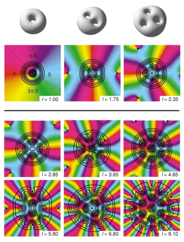
Figure 15: (Color online) Vortices in a rotating cloud of bosons. Schematically shown are the vortex holes that penetrate the boson cloud with increasing angular momentum. The lower panel shows the phase of the order parameter, and its density contours. (The black dots indicate the vortex positions). After  Butts and Rokhsar (1999).

As we discussed in detail in Sec. III.1, the effective mean-field potential in the Gross-Pitaevskii approach may break the rotational symmetry of the Hamiltonian to lower the energy. As a consequence, such a mean-field solution for the order parameter is not an eigenstate of the angular momentum operator and the solution may reflect the internal symmetry of the exact quantum state. Similar behavior has been observed also in density-functional studies of quantum dots Reimann and Manninen (2002), and is further discussed also in the review by  Cooper (2008).

Figure 16 shows the expectation value of the angular momentum of a bosonic cloud as a function of the angular velocity of the trap, as obtained from the Gross-Pitaevskii approach Butts and Rokhsar (1999). The discontinuities in $l=L/N$ correspond to the topological transformations of the rotating cloud that are associated with the occurrence of additional vortices, as discussed above.

In the purely harmonic trap, the oscillator frequency $\omega$ limits the angular rotation frequency $\Omega$, see Eq. (1). When both quantities finally become equal, the condensate is no longer confined, and the atoms fly apart.

Figure 16: Angular momentum per particle, $L/N$, as a function of the rotational frequency $\Omega/\omega$ of the trap. The discontinuities correspond to the transitions between different symmetries. The insets show the surfaces of constant density in a spherical trap for states with two and six vortices. $\gamma=(2/\pi)^{1/2}aN/\sigma_{z}$, $a$ being the scattering length and $\sigma_{z}$ the axial width of the ground state of a single particle in the trap. From  Butts and Rokhsar (1999).

IV.2.2 Vortex molecules and lattices in quantum dots

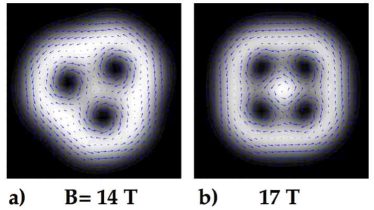
Figure 17: (Color online) Vortex molecules in a 6-electron droplet. Charge density (gray scale) and current density (arrows) show rotating currents around a) three and b) four localized vortex cores in density-functional calculations. After Saarikoski et al. (2004).

The close analogy between the bosonic ground state, $|N00000\cdots\rangle$ at $L=0$, and the fermionic maximum density droplet state, $|111\dots 111000\dots\rangle$ at $L_{\rm MDD}=N(N-1)/2$, (see Sec. II.6) suggests that vortex lattices may emerge also in fermionic systems to carry the angular momentum. Indeed, density-functional studies predicted the emergence of clusters or “vortex-molecule”-like geometric arrangements of vortices inside small droplets of electrons in quantum dots Saarikoski et al. (2004) when the angular momentum increases beyond the MDD. This happens in a very similar way as in bosonic droplets at small rotation frequencies Toreblad et al. (2004). An example of these vortex molecules in few-electron quantum dots is shown in Fig. 17. Figure  18 shows a cluster of 14 vortices in a 24-electron quantum dot calculated with the density-functional method in a local spin-density approximation (see Sec. III.2 above).

Figure 18: (Color online) Electron density (gray scale) and current density (arrows) in a 24-electron quantum dot calculated with the density functional method. The solution shows a cluster of 14 localized vortices arranged in two concentric rings. After Saarikoski et al. (2004).

These vortices correspond to off-electron nodes. The filling factor of the state in Fig. 18 can be approximated as $\nu\approx 0.63$. As in the bosonic systems vortex clusters are composed of single-quantized vortices Saarikoski et al. (2005b). Remarkably, the structure of the vortices that appear localized on two concentric rings with four vortices on the inner, and ten vortices on the outer “shell”, matches that of a classical Wigner molecule with 14 electrons at the verge of crystallization Bedanov and Peeters (1994). This also holds for the three- and four-vortex solutions shown in Fig. 17, where the triangle and square match the three- and four-particle classical Wigner-molecule configurations.

The clustering of vortices has also been analyzed with the CI method using reduced wave functions (see Sec. II.3.3) in the case of few-electron circular Saarikoski et al. (2004); Tavernier et al. (2004, 2006); Stopa et al. (2006) and elliptical Saarikoski et al. (2005b) quantum dots. In these studies the formation of few-vortex molecules has been found to follow a similar pattern in both the CI method and the density functional method.

Using the idea of the Bertsch-Papenbrock ansatz Bertsch and Papenbrock (1999) and assuming $n$ fixed vortex sites, we can anticipate that the single determinant describing a vortex ring would be Toreblad et al. (2004)

$$\Psi_{nv}=\prod_{j=1}^{N}\prod_{k=1}^{n}(z_{j}-ae^{i2\pi k/n})|\mathrm{MDD}\rangle=\prod_{j=1}^{N}(z_{j}^{n}-a^{n})|\mathrm{MDD}\rangle,$$ (47)

where $a$ is the radius of the ring of vortices. This wave function is not an eigenstate of the angular momentum, but it can be projected out by collecting the states with a given power of $a$ and symmetrizing the polynomial multiplying the $|\mathrm{MDD}\rangle$:

$$\Psi_{nv}=a^{n(N-K)}{\cal S}\left(\prod_{j=1}^{K}z_{j}^{n}\right)|\mathrm{MDD}\rangle,$$ (48)

where ${\cal S}$ is the symmetry operator and $K$ determines the average radius of the vortex ring. For example, with $N=7$, $K=5$ and $n=3$, the most important configuration is $|1100011111000\cdots\rangle$, in agreement with the CI calculations (in the LLL approximation) for vortex rings by Toreblad et al. (2004). We discuss localization and fluctuations of vortices further in Sec. IV.3.

Equation (48) also elucidates the origin of different vortex types and the similarity of fermion and boson systems. The zeros of the symmetric polynomial ${\cal S}(\prod z_{j}^{n})$ give the free vortices, while the zeros of $|\hbox{MDD}\rangle$ give the Pauli vortices. In a boson system, $|\hbox{MDD}\rangle$ is replaced with the boson condensate $|0\rangle$ which has no zeros, and only the free vortices appear, as illustrated in Fig. 19.

Figure 19: (Color online) Reduced wave function representation of of the vortex structure of the model wave function Eq. (48) for bosons and fermions ($N=7$, $n=2$, $K=2$). The fixed particles are shown as light dots, the current field with arrows (logarithmic scale) and the particle density as shades of red (light color corresponding to high density).

Studies of electron-vortex correlations in quantum dots indicate that, at least in few-electron systems, the electron-vortex separation $d_{\rm e-v}$ can be approximated by a universal quadratic function of the filling factor, $d_{{\rm e-v}}\sim d_{\rm e-e}\nu^{2}$, where $d_{\rm e-e}$ is the average electron-electron separation Anisimovas et al. (2008). This shows that in the limit of high angular momentum (low $\nu$) electrons tend to attract vortices closer to electron positions, which eventually leads to the formation of electron-vortex composites and the emergence of finite-size counterparts of the quantum Hall states.

The “rotating electron molecule” approach Yannouleas and Landman (2002, 2003) has also been used to analyze correlations between particles and vortices in electron droplets. However, this approach has been found to underestimate electron-vortex correlations Anisimovas et al. (2008) and vortex attachment to particles in the limit of high angular momentum Tavernier et al. (2004).

The vortex-molecule-like characteristics of the states are expected to vanish gradually with increasing vorticity. However, exact diagonalization studies of few-electron systems with Coulomb interactions have suggested that the above-described vortex ordering into Wigner-molecule-like shapes continues down to a filling factor $\nu={1\over 2}$, where the electron number equals the (off-electron) vortex number Emperador (2006). At $\nu={1\over 2}$ the structure of the state is complex Emperador et al. (2005) and possible electron pairing in this regime has been studied Harju et al. (2006); Saarikoski et al. (2008). This filling factor marks also the beginning of a regime $\nu<{1\over 2}$ where the vortex attachment to particles becomes pronounced Emperador (2006). We further discuss the breakdown of vortex molecules and the emergence of fractional quantum-Hall-liquid-like states in Sections IV.3 and IV.6, respectively.)

IV.2.3 Signatures of vortices in electron transport

For quantum dots in the fractional quantum Hall regime, where vortices have been predicted to form, electron transport measurements have revealed a rich variety of transitions associated with charge redistribution within the electron droplet Ashoori (1996); Oosterkamp et al. (1999).

Quantum dots contain a tunable and well-defined number of electrons. The electron transport experiments in the Coulomb blockade regime at low temperatures (around 100 mK) measure the chemical potential

$$\mu(N)=E(N)-E(N-1),$$ (49)

which gives the minimum energy needed to add one more electron to the electron droplet. Transitions in the electron transport data can be seen as cusps or jumps in the chemical potential. Different quantum Hall regimes can be identified from these characteristic features of the chemical potential as a function of both the electron number and the magnetic field, see Fig. 20.

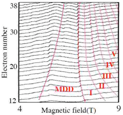
Figure 20: Current peaks in the electron transport experiments and transitions in the spin-density-functional theory (red lines). The dashed lines denote the MDD boundaries and the roman numerals indicate number of vortices in the theory. After Saarikoski and Harju (2005); the experimental data are from Fig. 2b in Ref. Oosterkamp et al. (1999).

In experimental studies of vertical quantum dots, a harmonic external potential has been found to give a good approximation of the confining potential Matagne et al. (2002). The harmonic confinement strength $\hbar\omega_{0}$ is determined by the size of the quantum dot device, and usually depends on the number of electrons $N$ inside the quantum dot. The area of the electron droplet has been found to increase with the gate voltage suggesting that the electron density in the droplet remains constant Austing et al. (1999b). Confining potentials scaling as $\hbar\omega_{0}\sim N^{-1/4}$ in Koskinen et al. (1997) or $\hbar\omega_{0}\sim N^{-1/7}$ in Saarikoski and Harju (2005) have been used in order to compare with experimental data.

The MDD state in quantum dots is the finite-size counterpart of the $\nu=1$ quantum Hall state. Its existence has been firmly established in experiments since it gives rise to a characteristic shape in the chemical potential at $\nu=1$ Oosterkamp et al. (1999). The MDD state assigns one Pauli vortex at each electron position giving a total magnetic flux of $N\Phi_{0}$. As the rotation is further increased, the MDD reconstructs Chamon and Wen (1994); Goldmann and Renn (1999); Reimann et al. (1999); MacDonald et al. (1993); Toreblad et al. (2006), and a vortex enters the electron droplet. This transition occurs approximately when the magnetic flux $\Phi=BA$ through the MDD of area $A$ exceeds $(N+1)\Phi_{0}$. Subsequent transitions involve an increasing number of such off-electron vortices Saarikoski et al. (2004); Toreblad et al. (2004). Assuming a constant electron density in the droplet, the change in $B$ required for the addition of subsequent off-electron vortices in the droplet is approximately $\Delta B=\Phi_{0}n/N$. This result can be compared to density-functional calculations, which indicates a $1/N$-dependence of the spacing between the first major transitions after the MDD state. However, the limited accuracy of the available electron transport data at present does not allow to draw any more firm conclucions.

The different ground states obtained within density-functional theory are compared to electron transport data in Fig. 20. The transition patterns in theory and experiment show a narrowing of the stability domain of the MDD.

Closer examination of the chemical potential for different $N$ values and comparison with the mean-field results reveal different quantum Hall regimes as the magnetic field is increased. Fig. 21 shows the chemical potential for $N=13$ and $N=30$.

Figure 21: Chemical potential of a quantum dot device with $N=30$ (upper panel) and $N=13$ (lower panel) compared to the results from the spin-density-functional theory. The experimental data are from Oosterkamp et al. (1999). Noise in the experimental data has been reduced by using a Gaussian filter. In the calculations the confining potential is assumed to be parabolic with $\hbar\omega_{0}$ being 4.00 meV for $N=13$ and 3.51 meV for $N=30$. Finite-size precursors of different quantum Hall states are identified. The roman numbers between the filled triangles indicate the number of vortices inside the electron droplet predicted by the density-functional calculations. The open triangles mark other possible transitions which are beyond the reach of density-functional theory.

The agreement with the electron transport data is best in the vicinity of the MDD domain. Experimental data show additional features not accounted for by the density-functional theory (open triangles in Fig. 21), which could be attributed to correlation effects, especially a transition to partially polarized states Oaknin et al. (1996); Siljamäki et al. (2002). In a Quantum Monte Carlo study by Güçlü et al. (2005) the frequency of transitions per unit of magnetic field was calculated in the $\nu<1$ regime and it was found to roughly correspond to the frequency in experiments. However, many of the calculated transitions give rise to small changes in angular momentum and energy. A direct comparison with experiments is therefore difficult due to noise in experimental setups and inevitable imperfections in the samples. Nishi and coworkers have done experimental measurements and detailed modeling for few-electron quantum dots Nishi et al. (2006). High-accuracy electron transport data that would go deep into the fractional quantum Hall regime, are still lacking for higher electron numbers.

Magnetization measurements of quantum dots could provide another way to probe for transitions caused by vortex formation inside electron droplets. Observed oscillations in the magnetic susceptibility $\chi=\partial M/\partial H$ have been analyzed, showing the de Haas–van Alphen effect in large arrays of quantum dots Schwarz et al. (2002). However, to resolve transitions in individual states in the regime of high angular momentum is challenging, because the shapes of the quantum dots in the ensemble must be sufficiently uniform, and the number of electrons in the samples has to be small.

IV.3 Localization of particles and vortices

We have seen above that localized vortices and vortex molecules have been observed in rotating bosonic systems, and very similar structures were predicted to occur in rotating fermion droplets. Vortex localization can be seen as analogous to particle localization within the framework of the particle-hole duality picture, discussed in Sec. II.4. We start this section by a brief discussion of particle localization in 2D systems. Insight and concepts derived from these studies are necessary as we proceed to discuss the analogy between particle and vortex localization.

IV.3.1 Particle localization and Wigner molecules

Wigner crystallization Wigner (1934) has been observed for electrons trapped at the surface of superfluid liquid helium Andrei et al. (1991) or in a two-dimensional electron gas in a semiconductor heterostructure Pudalov et al. (1993). Recent addition energy measurements of islands of trapped electrons floating on a superfluid helium film have revealed signatures of a Wigner-crystalline state Rousseau et al. (2009). In the low-density limit, the kinetic energy of the 2D electron gas becomes very small and the interparticle interactions dominate. The crystalline phase is expected to emerge at the density parameter $r_{s}\approx 37a_{B}^{*}$, where $a_{B}^{*}$ is the effective Bohr radius Tanatar and Ceperley (1989) ($r_{s}$ is a radius of a circle containing on average one electron). This estimate is in agreement with more recent computations by Attaccalite et al. (2002, 2003).

A finite system of a few (nearly) localized electrons is commonly referred to as a “Wigner molecule”. In small quantum dots, these Wigner molecules take the shapes of simple polygons, depending on the number of electrons that can be resolved by classical electrostatics Bolton and Rössler (1993); Bedanov and Peeters (1994). In the non-rotating case, the onset of electron localization occurs already at relatively high densities $r_{s}\approx 4a_{B}^{*}$ Jauregui et al. (1993); Egger et al. (1999); Reimann et al. (2000); Yannouleas and Landman (2007). In this context it is interesting to note that in small systems most of the particles localize at the perimeter of the dot. For seven electrons, for example, six particles localize at the vertices of a hexagon, with the seventh particle at the dot center Bolton and Rössler (1993): the electrons along the perimeter essentially form a 1D system where the localization is even easier than in 2D Kolomeisky and Straley (1996); Viefers et al. (2004). Localization in the radial direction takes place first followed by localization in the angular direction Filinov et al. (2001); Ghosal et al. (2006).

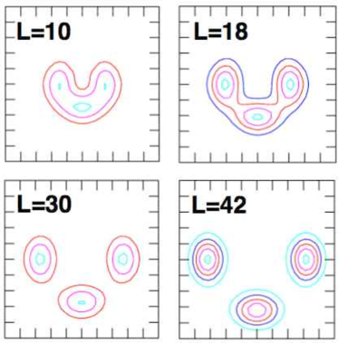
Figure 22: (Color online) Pair-correlation functions of four fermions with repulsive Gaussian interactions at four different angular momenta $L=10$, $L=18$, $L=30$, and $L=42$, respectively, showing that localization increases with rotation. The contour plots are in the same scale to demonstrate the expansion due to the rotation. From Nikkarila and Manninen (2007a).

In small electron systems there are no true phase transitions and the localization of electrons increases gradually with decreasing electron density Reimann et al. (2000). Inelastic light scattering experiments have only been used to probe excitations of molecule-like states in few-electron quantum dots in the high-density regime where, however, localization has not yet occured Kalliakos et al. (2008). Addition-energy spectra obtained from Coulomb blockade experiments Tarucha et al. (1996) have been proposed as a direct probe for signatures of localization Güçlü et al. (2008). In large quantum dots, the crystallization occurs in ring-like patterns, like the shells of an onion Filinov et al. (2001); Ghosal et al. (2006). A gradual rearrangement of addition energy spectra, which indicates a change in shell fillings, is then predicted to occur as the shell sizes of Wigner molecules differ from those of non-localized electrons. However, no experimental data yet exist in this regime.

Quantum dots are often modeled as circularly symmetric and the associated quantum states and ground-state electron densities therefore also have the same symmetry. The localization of particles takes place in the internal frame of reference. In the laboratory frame the localization is seen in the total density distribution only when using approximate many-particle methods which allow symmetry breaking, such as for example the unrestricted Hartree-Fock approach Yannouleas and Landman (1999). Other possibilities are to break the symmetry of the confining potential, as for example by an ellipsoidal deformation Manninen et al. (2001a); Saarikoski et al. (2005b); Dagnino et al. (2007); Dagnino et al. (2009b, a), or to analyze localization of the probing particle in the reduced wave function Harju et al. (2002); Saarikoski et al. (2004). However, there are other straightforward methods to see the localization in exact calculation for circular confinement: Figure 22 shows the pair-correlation function (conditional probability) for four particles at different values of the total angular momentum. Clearly, when the angular momentum increases, the particles are further apart and the localization becomes more pronounced. Another possibility is to study the rotational many-particle energy spectrum, which is more intricate, but also more revealing.

IV.3.2 Rotational spectrum of localized particles

When the particles are localized, we may consider the system as a rotating “molecule” with a given point group symmetry. In the case of two identical atoms in a molecule the rotational spectrum shows a two-fold periodicity in the angular momentum, which may be odd or even depending upon whether the atoms are bosons or fermions Tinkham (1964). Similarly, for $N$ identical particles forming a ring, only every $N$th angular momentum is allowed Koskinen et al. (2001) in a rigid rotation around the symmetry axis. For other angular momenta, the rotational state should be accompanied by an internal excitation. In the case of particles having no internal degrees of freedom (no spin), the only such excitations are vibrational modes of the molecule. Group theory can then be used to resolve the vibrational modes which are allowed to accompany a certain angular momentum eigenvalue Maksym (1996); Koskinen et al. (2001); Viefers et al. (2004).

Plotting the energies of the many-body system as a function of the angular momentum, the lowest energy (yrast line) has oscillations with a period of the symmetry group. The minima correspond to pure rotational states. Between the minima the states have vibrational excitations which increase the energy. Maksym showed that the energy spectrum of few electrons at high angular momenta can be quantitatively explained by a rotating and vibrating Wigner molecule Maksym (1996) which is the basis for the molecular approaches to correlations in quantum dots Maksym et al. (2000) and quantum rings Koskinen et al. (2001). Several other studies have later confirmed this observation, for a review see Viefers et al. (2004). This molecular approach for rotating particles has also been used by Yannouleas and Landman (2002, 2003), who introduced “rotating electron molecule” wave functions to describe rotating molecular states at high angular momenta. These wave functions are available in analytic form, with their internal structure constructed by placing Gaussian functions at classical positions of electrons in high magnetic fields.

Formulating a molecular model of a rotating system, we may approximate the many-particle spectrum (at zero magnetic field) by

$$E=\frac{L^{2}}{2I_{L}}+\sum_{\nu}\hbar\omega_{L\nu}\left(n_{\nu}+\frac{1}{2}\right),$$ (50)

where $I_{L}$ is the moment of inertia of the Wigner molecule and $\omega_{L\nu}$ the vibrational frequencies. $I_{L}$ and $\omega_{L\nu}$ can be determined using classical mechanics in the rotating frame, and thus depend on the angular momentum as indicated with the subscript $L$. The eigenenergies Eq. (50) can be compared to those calculated from the exact diagonalization method.

To give an example for the signatures of localization in the many-body energy spectra, Fig. 23 shows the rotational three-particle spectrum. A broad range of low-lying states may be described quantitatively with the rotation-vibration model of Eq. (50).

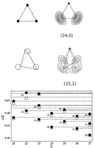
Figure 23: Classical orbits and pair-correlation functions of localized electrons in rotating frame (upper panel). At angular momentum $L=24$ the lowest energy state is purely rotational while at $L=25$ a doubly excited rotational state is shown. In the rotating frame the classical motion shows a pseudo-rotation (middle left) while the pair-correlation shows maxima at the classical turning points (middle right).The spectrum (lower panel) compares the exact energies (dots) with those of the classical model (squares). It shows a periodicity of $\Delta L=3$ in angular momentum, which agrees with the localization in a triangular geometry (see upper panel). The horizontal dashed lines indicate the center-of-mass excitations which occur at all angular momenta. From Nikkarila and Manninen (2007b).

Figure 23 also shows examples of the pair-correlation functions for a purely rotating state and for a state including vibrational modes. Similar observations have been reported for other vibrational modes and particle numbers Maksym et al. (2000); Nikkarila and Manninen (2007a). A more detailed quantum-mechanical analysis of the molecular states has recently also been reported by Yannouleas and Landman (2009).

Finally, we should consider what happens to the rotational energy spectrum when the particles have internal degrees of freedom, say spin. In the classical limit, the internal degrees of freedom separate from the spatial excitations (vibrations), since the Hamiltonian is spin-independent. The different spin-states of the system will eventually become degenerate. However, the existence of the different spin states will give more freedom to satisfy the required symmetry (bosonic or fermionic) of the total wave function. Again, group theory can be used to determine the spin states which are allowed for a given angular momentum and a given vibrational state Maksym (1996). The energies agree well with the classical model of Eq. (50) Koskinen et al. (2007).

The localization of the particles may in fact also be incomplete. This is indicated by the non-vanishing particle density in between the classically localized geometries, as well as small deviations in the symmetry of the Wigner crystal. Especially the excited quantum Hall states (edge states) may show such structures, as discussed already in connection with vortex formation, see Sec. IV.1. The lowest-lying excitations of a large electron droplet above the MDD state have been predicted to show particle localization into rings of electrons around a compact non-localized core of the MDD electrons  MacDonald et al. (1993); Chamon and Wen (1994). The wave functions of these states contain a single node at a finite distance from the center (i.e., a non-localized vortex, see Sec. IV.1.3) which leads to a separated ring of localized electrons at the edge, often referred to as the Chamon-Wen edge, that has been much discussed in the literature Goldmann and Renn (1999); Reimann et al. (1999); Manninen et al. (2001a); Reimann and Manninen (2002); Toreblad et al. (2006). The localized edge state appears when the MDD begins to break up with the entrance of the first vortex, but before further vortex holes penetrate the cloud (see Sec. IV.3.4). It should be noted that the current-spin-density functional theory Vignale and Rasolt (1987, 1988) with the local density approximation Reimann et al. (1999) largely over-emphasizes the localization of electrons in the Chamon-Wen edge Toreblad et al. (2006).

IV.3.3 Localization of bosons

In a non-rotating condensate, all bosons may occupy the same quantum state. In the regime of high angular momenta, however, rotation may induce localization in bosonic systems in the same way as in fermionic systems. In both cases, the rotation pushes the particles further apart, and the classical picture of a rotating and vibrating Wigner molecule Maksym (1996) sets in. The similarity of bosons and fermions in reaching the classical limit was suggested by Manninen et al. (2001b) on the basis of Laughlin’s theory Laughlin (1983) of the fractional quantum Hall effect, and has been subsequently studied more quantitatively: a detailed comparison of few bosonic and fermionic particles in a harmonic trap Reimann et al. (2006a) indicated similar localization effects in both systems. Note that for small particle numbers in the LLL, the mapping between boson and fermion states, discussed in Section II.4, becomes increasingly accurate when the angular momentum increases Borgh et al. (2008), in accordance with the classical interpretation of the spectrum.

IV.3.4 Vortex localization in fermion droplets

There is an apparent analogy between vortex localization and particle localization: we have seen above that localized vortices cause minima in the electron density, with rotational currents around their cores. These “holes” arrange in vortex molecules, with shapes that indeed resemble those of Wigner molecules in the case of particle localization, discussed in Sec. IV.3.1. (Note that the Pauli vortices do not give rise to vortex structures in the electron density, since each electron carries one such vortex).

The vortex localization can be illustrated by the configuration mixing of the exact quantum states. If the configuration has, say, four vortices and $|11110000111111\cdots\rangle$ has the largest weight, other configurations with the same angular momentum, like $|11101001011111\cdots\rangle$, have a finite weight. The CI method shows that the mixing of these states happens mostly around the holes in the filled Fermi sea, as indicated in Fig. 24. This means that the holes are strongly correlated and may localize.

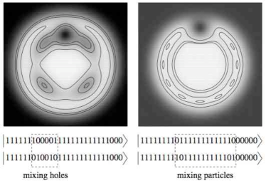
Figure 24: Electron-electron pair-correlation functions showing localization of four vortices (left) and localization of electrons at the edge of the cloud in the case of one vortex (right). White color means high density, and some constant-density contours are shown. The two most important configurations are given in each case, demonstrating that mixing of single-particle states close to holes leads to hole localization, while correspondingly the mixing of particles localizes particles. The results are calculated with the CI method for 20 particles with angular momenta $L=202$ (left) and $L=242$ (right).

This can be directly compared to the localization of particles. As discussed further in Sec. IV.3.1, the lowest-lying excitations of a large electron droplet above the MDD state were predicted to show particle localization into ring-like geometries, with a single vortex hole at a finite distance from the center (see Sec. IV.1.3). In this case, the configuration mixing is shifted to the outer edge of the droplet where it leads to a ring of strongly correlated particles, as for example seen in Fig. 24.

The localization of particles and vortices in a circular system breaks the internal symmetry (unless a single vortex is localized at the center). The density functional method, using a local approximation for the exchange-correlation effects, may show the localization of particles and vortices directly in the particle and current densities (see Fig. 18 and discussion of symmetry breaking in Sec. II.1.3), as discussed above. However, the true many-body wave function of the system must have the symmetry of the Hamiltonian. Figure 24 already demonstrated that the localization of vortices can be seen in the pair-correlation functions by taking the reference point to be at the same radius as the vortices. Moreover, in a one-component fermion system, particle-hole duality (see Sec. II.4) can be used to gain insight into correlations between vortices. Transformation of a bosonic wave function to a fermionic one can be used to illustrate the vortex localization. Any fermion state can be written as a determinant of the MDD times a symmetric polynomial, where vortex structures are included in the latter Manninen et al. (2005). On the other hand, this polynomial is a good approximation to the exact boson wave function, as discussed in Sec. II.6.

Figure 25 shows examples of the particle-particle and hole-hole correlation functions which indeed reveal that vortices in both boson and fermion systems are well localized.

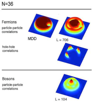
Figure 25: (Color online): Pair-correlation functions for large fermion and boson systems with four vortices. The pair-correlation function of the MDD is displayed for comparison; it only shows the exchange-correlation hole at the reference point.

This can be understood by considering the angular momentum of the system of holes, and the corresponding filling factor of the LLL. For example, in the case of four vortices, the hole filling factor is as low as about 1/9, which corresponds to the value where the particles form a Wigner solid in an infinite system. In other words, when the electron filling factor approaches unity (from below), the hole filling factor approaches zero, forcing the holes to be localized.

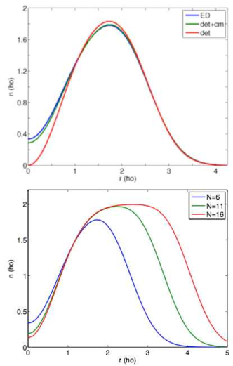
Figure 26: (Color online) Upper panel: Radial electron densities in a harmonic trap ($\omega=1$) in a six-electron droplet with a central vortex at $L=21$ (in harmonic oscillator units). The exact solution in the LLL is shown by the blue line, a single-determinant wave function which describes a central vortex is shown by the red line, and a single-determinant wave function in the center-of-mass (CM) transformed coordinates $z_{i}\to z_{i}-z_{\rm CM}$ is shown by the green line. Lower panel: Radial electron densities for central vortex states $L=L_{\rm MDD}+N$, showing that vortex localization increases with electron number $N$ due to decrease in the center-of-mass motion.

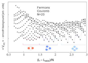
Figure 27: (Color online) Fermion low-energy spectrum for 20 particles. The lowest energy many-particle states as a function of the total angular momentum (yrast states) are connected with lines to guide the eye. A smooth function of angular momentum was substracted from the energies to emphasize the oscillatory behavior of the yrast line. The periodicity of the oscillation reveals the number of localized vortices as schematically illustrated. From Reimann et al. (2006b).

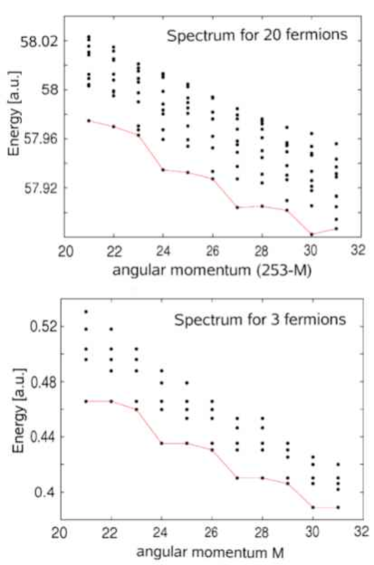
Figure 28: Fermion yrast spectrum for 20 particles and three vortices (upper panel) and 3 particles (lower panel) show both the periodicity of $\Delta L=3$ associated with the three-fold rotational symmetry of the vortex molecule in the former case and electron molecule in the latter case. From Manninen et al. (2006).

Hole-hole correlations in Fig. 25 show clearly the effect of the zero-point fluctuation in the vortex position. To examine this further in the case of fermions, let us as an example investigate the singly-quantized vortex for six electrons in a harmonic confinement. As discussed earlier in Sec. IV.1.3 the MDD state in this case, with angular momentum $L=15$, is characterized by a relatively flat electron density. The electrons occupy the six lowest levels of angular momentum in the lowest Landau level with occupancies $|11111100\ldots\rangle$. When the angular momentum increases, at stronger magnetic fields the MDD state is reconstructed and a vortex hole is created in the center. This state has angular momentum $L=21$. The single-particle determinant $|011111100\ldots\rangle$ with a weight 0.91 yields the largest contribution to the wave function in the lowest Landau level. Due to fluctuations, the exact many-body wave function includes other single-particle determinants corresponding to $L=21$, such as $|1011110100\ldots\rangle$ and $|11011100100\ldots\rangle$. However, since their weights are relatively small, the state can be characterized by a rather flat maximum density droplet configuration with a vortex hole in the center. The electron density of this state, indeed, shows a deep hole in the center and a rotating current around it (upper panel of Fig. 26). Fluctuations in the vortex position cause the particle density to remain finite in the center of the confining potential. A single-determinant wave function $|01111100\ldots\rangle$ transformed into the center-of-mass coordinates $z_{i}\to z_{i}-z_{\rm CM}$ shows a density profile that is very close to the exact results (upper panel of Fig. 26). The quantum mechanical zero-point motion of the vortex hole leads to a finite density at the vortex core. The center-of-mass fluctuations decrease with electron number, which is reflected by localization increasing with particle number (lower panel of Fig. 26).

IV.3.5 Vortex molecules

A section of the many-particle energy spectrum for $N=20$ electrons for different angular momenta $L$ is shown in Fig. 27 Reimann et al. (2006b). The yrast line shows periodic oscillations, with the oscillation length (in units of $L$) equal to number of localized vortices in the system. The reason behind these periodic oscillations in the energy spectrum is deeply connected with the above-mentioned particle-hole duality and vortex localization: they are signatures of two, three, and four vortices, respectively, being localized at the vertices of simple polygons with $C_{2v}$ symmetry. For polarized fermions as in Fig. 27, the rigid rotation of the vortex “molecule” with $n$-fold symmetry is allowed only at every $n^{th}$ angular momentum, corresponding to a minimum (cusp) in the yrast line. At intermediate angular momenta, the rigid rotation is accompanied by other excitations, such as vibrational modes, that result in higher energies Nikkarila and Manninen (2007a). Figure 28 compares a small part of the spectrum to that for three electrons. The marked similarity of these spectra demonstrates not only that the vortices are localized in a triangle, like the three electrons, but also that elementary excitations of the many-particle energy spectrum are vibrational modes of the vortex-molecule.

Under certain circumstances the particle and current densities of the (exact) many-body state may show directly the formation of vortex molecules. This may for example be the case for a broken rotational symmetry of the system, as for example predicted for elliptically confined quantum dots Manninen et al. (2001a); Saarikoski et al. (2005b). Fig. 29 shows the electron density of an elliptical 6-electron quantum dot calculated by exact diagonalization.

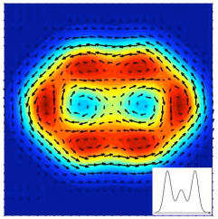
Figure 29: (Color online) Electron density (color, with red for maximum density) and current density (arrows) of an elliptically confined 6-electron droplet with two localized vortices, calculated by the exact diagonalization method. The confinement strength is $\hbar\omega_{0}=5.93\;{\rm meV}$, the eccentricity of the elliptic confining potential $\delta=1.2$ and the magnetic field is $B=17$ T. Inset: profile of the electron density at the longest major axis shows fluctuations in the vortex positions, which causes electron density to remain finite at the density minima. Adapted from Fig. 6 in Saarikoski et al. (2005b).

Two localized vortices can be identified as minima in the charge density, around which the current shows the typical loop structure. In highly excentric confining potentials, vortex structures containing three and more localized vortices were also predicted to form Saarikoski et al. (2005b). The effect of fluctuations in the vortex positions is clearly seen also in this case. To some extent, electron localization is observed as well. In this case, the wave function can be characterized by two hole-like quasi-particles at the center of a ring of six electrons. It should be noted that Fig. 29 shows the exact particle density, and not the mean-field particle density. Since elliptically deformed quantum dots have been realized experimentally Austing et al. (1999a) this may be the most direct way to image vortex structures in quantum dots. Localized vortex structures have been predicted to emerge also in other quantum dot geometries Saarikoski et al. (2005b); Marlo-Helle et al. (2005).

A perturbative approach to visualize vortices in the particle density is to include a point-perturbation in the external potential Christensson et al. (2008b), which can pin the vortices. The resulting particle density clearly shows the vortex localization. An example is shown in Fig. 30 for a system of 8 electrons. With this small perturbation, the expectation value of the angular momentum still has a nearly similar dependence on the rotational frequency than the unperturbed system. It is thus expected that each angular momentum jump in the nonperturbed system corresponds to addition of one vortex as seen in the perturbed system.

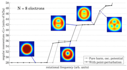
Figure 30: (Color online) Angular momentum as a function of the rotational frequency of the parabolic trap with $N=8$ electrons in the lowest Landau level. The unperturbed result (thin line) is comparable to the expectation value of angular momentum in the presence of an added point perturbation which breaks the rotational symmetry (thick solid line). The insets show the densities in the perturbed system. The vortices appear as pronounced minima in the density distribution, their number increasing with the trap rotation. Results are calculated with the exact diagonalization method Christensson et al. (2008b).

IV.4 Melting of the vortex lattice

After single vortex lines in rotating condensates were experimentally realized by phase imprinting techniques Matthews et al. (1999), many experimental studies concerned the formation of lattices of vortices in bosonic cold-atom gases in the regime of high particle-to-vortex ratio (filling factor) $\nu_{pv}=N/N_{v}$  Chevy et al. (2000); Madison et al. (2000, 2001). The modes of the vortex lattice Baym (2003, 2004) as well as the structure of the vortex cores were analyzed Coddington et al. (2003); Schweikhard et al. (2004); Coddington et al. (2004). When the vortex density increases with the angular momentum, it is expected that for rapid rotation, the vortex density may finally become comparable to the particle density Ho (2001); Fetter (2001); Cooper et al. (2001). An interesting issue is then how the system changes with the increasing particle-to-vortex ratio Baym (2005). At rapid rotation, strongly correlated states analogous to fractional quantum Hall states may emerge Wilkin et al. (1998); Viefers (2008); Cooper (2008). These states are quantum liquid-like states of particles and vortices where correlations may give rise to the formation of particle-vortex composites. It is believed that a phase transition occurs with a vortex density somewhere between the rigid vortex lattice and the quantum liquid of vortices. This transition is often refered to as “melting”. However, the process is not fully understood and calculations yield different estimates for the critical vortex density. Moreover, in present day experiments the particle-to-vortex density is usually very high, $\nu_{pv}\gtrsim 500$ Schweikhard et al. (2004).

IV.4.1 Lindemann melting criterion

The vortex density at the transition from localized vortex lattice states to liquid-like states can be approximated by assuming that the melting process is analogous to the melting of solids when atomic vibrations increase above a threshold amplitude. In the Lindemann model the melting point of solids is determined from the condition that when thermal vibrations reach a critical amplitude, melting of the material occurs Lindemann (1910). This amplitude in solids is often approximated to be around 10% to 20% of the lattice spacing. Using an analogous idea, the melting point of the vortex lattice can be approximated from the condition that thermal and quantum zero-point vibrations reach a critical threshold amplitude Blatter and Ivlev (1993).

Rozhkov and Stroud (1996) studied the vortex lattice melting in superconductors at zero temperature to obtain an estimate for the vortex density where zero-point fluctuations become large enough to melt the vortex lattice. Their study was motivated by the presence of large quantum fluctuations in high-$T_{c}$ materials but their results give also an estimate of the vortex lattice melting in ultra-cold rotating Bose-Einstein condensates. Using the Lindemann criterion they approximated that melting takes place at particle-to-vortex filling factor $\nu_{pv}\sim 14$ at a presumed threshold zero-point vibration amplitude of 14% of the nearest-neighbour inter-vortex distance.

Other calculations using the Lindemann criterion have given comparable estimates of the filling factor at the vortex lattice melting (see also the discussion in the reviews by Cooper (2008) and Fetter (2009)). Sinova et al. (2002) reported that the critical density in their model system of rapidly rotating bosons corresponds to $\nu_{pv}\sim 8$. Baym (2003, 2004, 2005) analyzed normal modes of vortex lattice vibrations in the mean-field limit and found that the vortex lattice melts at $\nu_{pv}\sim 10$.

IV.4.2 Transition to vortex liquid state

The predictive power of the Lindemann model is poor because melting in solids is known to be a co-operative phenomenon, and the process therefore cannot be accurately described in terms of the mean vibration amplitude of a single particle. However, Rozhkov and Stroud (1996) obtained another estimate $\nu_{pv}\sim 11$ for the melting point of the vortex lattice by comparing the energy of a Wigner crystal model wave function to the energy of a Laughlin-type wave function. These wave functions were assumed to correspond to the ordered vortex-lattice state and the vortex-liquid state, respectively. Exact diagonalization calculations with contact interactions in a periodic toroidal geometry showed that the excitation gap collapsed at $\nu_{pv}\sim 6$, which was interpreted as a lower bound for a vortex lattice melting Cooper et al. (2001). The associated vortex-liquid states at integer and half-integer $\nu_{pv}$ were in this work shown to be, in general, well described with so-called parafermion states studied by Read and Rezayi (1999).

In contrast to bosonic systems, the vortex lattice melting has not been studied theoretically in fermion systems. However, we can obtain an estimate for a corresponding transition using the particle-hole duality (Sec. II.4). There is a transition from the fractional quantum Hall liquid to localized electrons (i.e. the formation of a Wigner crystal) when the filling fraction of the LLL decreases below $\nu\approx 1/7$ Lam and Girvin (1983); Pan et al. (2002). There are about 6 to 8 vortices per particle, not counting the Pauli vortices, at the transition point. Using the particle-hole duality we can now reverse the role of particles and vortices. In the dual picture a lattice of localized vortices then melts to a quantum Hall liquid when the particle-to-vortex ratio decreases to a value between 6 and (about) 8. This corresponds to a filling factor between $\nu\approx 0.8$ and $0.9$, where a vortex lattice is expected to melt in a 2DEG. The close relation between boson and fermion states in the LLL, Eq. (21), would suggest that also in boson systems the vortex lattice should melt when the particle-to-vortex ratio decreases to about $8$, which is not too different from the values mentioned above.

In conclusion, even though the results of different calculations show a considerable variation for the melting point, they all indicate vortex lattice melting well before the number of vortices in the system becomes comparable to the particle number. However, much of the details are not understood, and experiments do not yet reach the transition regime. The transition may happen gradually and go through several intermediate states with increasing vortex delocalization, or, as the name explicitly suggests, it may occur through an abrupt loss of vortex ordering.

IV.4.3 Breakdown of small vortex molecules

As discussed earlier, rotation in the intermediate angular momentum regime in small quantum droplets may give rise to formation of vortex molecules which are analogues of vortex lattice states of infinite systems. However, in finite-size systems, edge effects may play an important role. This was noted also in the context of Wigner crystallization in quantum dots, where the onset of localization occurs at electron densities which are much higher than the corresponding values for the infinite 2D electron gas. The importance of edge effects has been pointed out also for bosonic systems Cazalilla et al. (2005).

Partly, localization effects account for the fact that in small systems also the $\nu=1/3$ state appears localized, as for example visible in the pair-correlation functions. The same applies to vortices, and in very small systems it is difficult to make a difference between a vortex molecule and a vortex liquid, since both show similar short-distance correlations.

The analysis of few-electron quantum dots using the exact diagonalization method has shown that the final break-up of vortex molecules and the transition into the fractional quantum Hall regime of electrons is associated with the formation of composites of particles and vortices Saarikoski et al. (2004). Electrons “capture” free vortices, breaking up the vortex molecules. Similar processes have been reported also for bosons in the LLL by analysing the vortex attachment with reduced wave functions (see Fig. 31).

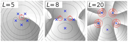
Figure 31: (Color online) Reduced wave functions of a bosonic 5-particle system in a harmonic trap, showing the formation of one and two free vortices in the region of high particle density (marked as circles) at low angular momenta $L=5$ and $L=8$, respectively (left and middle). When the angular momentum increases, two vortices are finally captured by each particle to form a state which is approximated by the bosonic Laughlin state $m=2$ (two concentric circles) at $L=20$ (right). Particle interactions are Coulombic here and the probe particle is at the bottom. After Suorsa (2006).

These calculations suggest, however, that vortices continue to show ordering at surprisingly low particle-to-vortex filling factors, well below the obtained stability limits of vortex lattices in bosonic condensates. This is also evident for fermions, as shown in Fig. 24, where hole correlations show vortex molecules at very high angular momentum and large zero-point fluctuations. In the case of fermions, vortex localization may continue to filling factors down to $\nu={1\over 2}$ where a transition from prominent vortex localization into particle localization occurs Emperador (2006). These calculations showed signs of vortex-hole bunching and the formation of concentric rings of localized vortices, until the number of (free) vortices was equal to the number of particles. Below $\nu={1\over 2}$, no such signatures are seen. Instead, this regime is characterized by particle localization. The conditional probability densities begin to show prominent localized structures Koskinen et al. (2001); Yannouleas and Landman (2007). The corresponding bosonic case has not been studied, but due to close analogies of bosonic and fermionic states, similar results are expected to hold also for small bosonic droplets where vortex localization should disappear at $\nu_{pv}=1$.

These results suggest that signatures of vortex localization in small systems disappear at a particle-to-vortex ratio which is an order of magnitude lower than the value where vortex lattice melting occurs in large bosonic condensates. However, as mentioned before, in small systems the separation of liquid and solid is difficult, and the observed transition is also related to the formation of composite particles (see Sec. IV.6).

IV.5 Giant vortices

In multiply-quantized vortices, the phase changes several integer multiples of $2\pi$ when encircling the singularity. However, they are not stable in a purely harmonic confinement potential. The existence of many singly-quantized vortices is energetically prefered, and the effective repulsive interaction between the vortex cores leads to a lattice of singly-quantized vortices Butts and Rokhsar (1999); Castin and Dum (1999); Lundh (2002). The instability of multiply-quantized vortices in harmonic potentials, and the break-up into singly-quantized vortices was further discussed by Möttönen et al. (2003) and Pu et al. (1999). Disintegration of a multiple quantized vortex has also been observed experimentally Shin et al. (2004).

Rotating condensates in anharmonic potentials that rise more rapidly than $r^{2}$, however, show a behavior that is very different from purely harmonic traps. Most commonly, a quartic perturbation is added to the oscillator confinement. Due to the anharmonicity it is possible to rotate the system sufficiently fast such that the centrifugal force may create a large density hole at the trap center. So-called “giant” vortices with a large core at the center may exist that originate from multiple quantization. Singly-quantized vortices may also form a close-packed ensemble inside a large density core. In addition, for certain parameter ranges, the usually-quantized lattice exists. Kavoulakis and Baym (2003) found a very rich phase diagram, for which a schematic picture is given in Fig. 32, showing the different possible phases as a function of the interaction strength and the trap rotation.

Figure 32: Schematic phase diagram of the ground states of a bosonic cloud in an anharmonic confinement. From Kavoulakis and Baym (2003).

In the following, we discuss the formation and structure of such “giant” vortex states in both bosonic as well as in fermionic quantum droplets.

IV.5.1 Bose-Einstein condensates in anharmonic potentials

Lundh (2002) proposed that in the presence of anharmonicity of the confining trap potential, multiply-quantized vortices with a giant vortex core could exist in a rotating condensate, and calculated the ground-state vortex structures within the Gross-Pitaevskii formalism. In fact, vortices in these states are not truly multiple-quantized vortices but rather dense-packed ensembles of single-quantized vortices Fischer and Baym (2003); Kasamatsu et al. (2002). Phase singularities do not completely merge into the same point because the residual interaction between phase singularities is logarithmic as a function of intervortex separation in the region of low particle density surrounding the cores. Despite this fact, the composite core has a large and uniform spatial extent. Therefore, the name “giant vortex” was coined for these structures. Depending on the strength of the anharmonicity, the condensate can exist in a phase where only single-quantized vortices occur, in a state where all vortices form a giant vortex, and in a mixed phase where both giant vortices and single-quantized vortices exist Kasamatsu et al. (2002); Kavoulakis and Baym (2003); Jackson et al. (2004); Jackson and Kavoulakis (2004). An example of the latter is shown in Fig. 33.

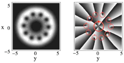
Figure 33: (Color online) A rotating Bose-Einstein condensate in a mixed state with a giant vortex in the center, surrounded by ten single-quantized vortices. The giant vortex is composed of four phase singularities. The left panel shows the particle density (white is high density and black is zero density) and the right panel shows the phase profile. Locations of phase singularities are marked with red circles. The large circle marks the ensemble of four phase singularities in the core of the giant vortex. After Kasamatsu et al. (2002), who applied the Gross-Pitaevskii method.

We further note that anharmonicity, which is required for giant vortex formation, may be induced also via the presence of another, distinguishable particle component. The interaction between the particles would then create an effectively anharmonic potential for the particle components which may induce giant vortex formation Bargi et al. (2007); Christensson et al. (2008a); Yang et al. (2008). This is discussed in Sec. V in the context of multi-component quantum droplets.

IV.5.2 Giant vortices in quantum dots

Giant vortex structures are predicted to form also in fermionic droplets with repulsive interactions, as it was shown by exact diagonalization calculations for few-electron quantum dots Räsänen et al. (2006). Similarly to the bosonic case, giant vortices emerge in anharmonic confining potentials and their structure shows a large core with multiple phase singularities. It was found that even a slight anharmonicity in the confining potential is sufficient for these giant vortex states to become energetically favorable. In addition to the particle interactions, fluctuations tend to keep phase singularities separated, broadening the charge deficiency in the core to a larger area (see Fig. 34). The electron density of a central giant-vortex state shows a ring-like distribution.

Figure 34: (Color online) A giant vortex in a six-electron quantum dot calculated with the exact diagonalization method. The left panel shows the particle density (black is low density) and current density (arrows), and the right panel shows the reduced wave function, where phase singularities are marked with red circles and electron positions with crosses. The giant core in this case comprises three phase singularities. Interactions and fluctuations keep the phase singularities separated. The probe electron is on the bottom-right. From Räsänen et al. (2006).

Unlike bosonic systems, giant vortices with repulsive fermions were only found in the limit of small numbers of particles. This could be seen as another manifestation of the tendency of vortices to drift towards the edge of the droplet in the limit of large particle numbers (see Sec. IV.1.3), breaking apart the giant vortex pattern at the center. In electron droplets interacting via Coulomb forces, density-functional calculations predicted that giant vortex formation is generally limited to systems with less than 20 fermions Räsänen et al. (2006).

IV.6 Formation of composite particles at rapid rotation

In the regime of high vorticity, electron-vortex correlations are particularly strong and cause vortices to be bound to electrons. This regime is ultimately linked with the fractional quantum Hall effect in the 2D electron gas. Actually, the early works aiming to explain this effect used a disk geometry Laughlin (1983); Girvin and Jach (1983) and are in fact more relevant for quantum dots than for the bulk properties of quantum Hall systems.

Figure 35 shows the nodal structure of the reduced wave function for the Laughlin state state for $N=5$ electrons as well as the corresponding $L=30$ state obtained with the CI method. In the Laughlin $\nu={1\over 3}$ state, there are three vortices on each electron position, one Pauli vortex and two extra vortices, as shown in Fig. 35(a). In the exact wave function, there are clusters of three vortices near each electron (except near the probe electron). There is one vortex on top of each electron position, as required by the Pauli principle, but, in addition, there are two vortices very close-by, separated by their mutual repulsion to opposite sides. Calculations show that small changes in the position of one of the fixed electrons in the reduced wave function causes the vortex to be dragged along with the electron, which indicates vortex attachment to the electron. The overlap between the exact state and the Laughlin approximation is 0.98. The state can be interpreted as a finite-size precursor of the $\nu={1\over 3}$ fractional quantum Hall state, for which the Laughlin wave function yields an accurate description. However, in contrast to the Laughlin state, the attachment of nodes to particles in the exact wave function shows a small spatial separation.

Figure 35: (Color online) The reduced wave functions for (a) the approximate Laughlin state $\nu={1\over 3}$ and (b) the exact $L=30$ ground state for five electrons in a parabolic external potential. The Laughlin state fixes a triple-vortex (concentric rings) on each electron position (crosses). In the exact solution there are clusters of three vortices near each electron.

The attachment of vortices to particles explains also the absence of vortices for the probe electron in the exact many-body state, see Fig. 35. In the fractional quantum Hall regime, the density-functional method failed to reveal the correct nature of the ground state. The solutions of the spin- as well as current-spin-density-functional theory show only a cluster of vortices inside the electron droplet, but these methods are unable to associate two extra vortices to each electron Saarikoski et al. (2005a) (see Fig. 36).

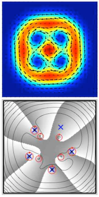
Figure 36: (Color online) A $\nu={1\over 3}$ state of five electrons in a harmonic trap. Left: electron density (color) from the density-functional method and current density (arrows). The confinement strength is $\hbar\omega_{0}=5\;{\rm meV}$ and the magnetic field is $B=18T$. Right: reduced wave function for the same state constructed from the Kohn-Sham single-particle states. The probe electron is at the top-right.

The density-functional approach fails to properly include these correlations. A single-determinantal wave function constructed from the self-consistent Kohn-Sham orbitals yields an approximate description for few-vortex states near $\nu=1$, but the overlaps with the exact wave functions diminish as the angular momentum of the system increases. Fig. 37 shows that for a five-electron system at $\nu=1/3$ the overlap is only of the order of 0.5 . Compared to this, the overlap with the Laughlin $\nu=1/3$ wave function that amounts to 0.98 is very high.

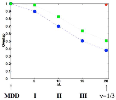
Figure 37: (Color online) Overlap of a single-determinant wave function with the exact one as a function of the angular momentum increase with respect to the MDD state $\Delta L=L-L_{\rm MDD}$ for 5-electrons in parabolic confinement. The higher points (squares) are obtained with a coordinate transformation to the center-of-mass, $z_{i}\to z_{i}-z_{\rm CM}$ and the lower ones (circles) without it. The star at $\Delta L=20$ shows the overlap with the Laughlin $\nu=1/3$ state. The roman numbers count the vortices inside the electron droplet. From Harju (2005).

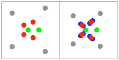
Figure 38: (Color online) Schematic view of the sites of vortices, determined from the reduced wave function of an exact diagonalization for five electrons with angular momentum $L=16$ (6 above the MDD, left) and $L=36$ (6 above the state with filling factor 1/3, right). Fixed electron positions with Pauli vortices are denoted by red bullets, vortices attached to electrons making composite particles by blue, and free vortices inside the electron droplet by green bullets. Free vortices outside the droplet are shown by gray bullets.

When the angular momentum of the droplet increases further, additional vortices appear in the Laughlin-like state and the filling factor decreases below $\nu=1/3$. These vortices are not bound to composite particles, rather they correspond to the Laughlin excitations with fractional charge. The pattern of vortex formation is expected to be similar to that after the MDD: first a single vortex enters from the surface and moves towards the center until it is energetically favorable to have two vortices, and so on. This is illustrated in Fig. 38, which shows the vortex sites for a five-electron system determined from the reduced wave function. Again, a similar behavior is expected in the case of bosonic particles. However, despite the recent progress in realizing BEC’s at extreme rotation Lin et al. (2009), an analysis of these states appears still to be beyond the current experimental capabilities.

There are two basic mechanisms to unbound the vortices from the particles, namely the softening of the interaction potential by e.g. the finite thickness of the system, and secondly by impurities. When the system has a finite thickness, the incompressible $\nu=1/3$ Laughlin state breaks down as the vortices are gradually less bound to the electron coordinates. This effect is in contrast to the screening of the Coulomb interaction energy whereby, in the strong-screening limit, the zeros are exactly localized to the electron positions Tölö and Harju (2009). We should also mention that repulsive impurities attract vortices at the impurity position Baardsen et al. (2009).

V Multi-component quantum droplets

Multi-component quantum droplets are composed of different particle species, that may for example be different atoms, different isotopes of the same atom, different spin states of an atom or electron, or even different hyperfine states of an atom. In such systems inter-component interactions can modify the many-body wave function significantly.

The properties of multi-component BEC’s have been much discussed, both experimentally and theoretically, over the past few years. For recent reviews on multi-component BEC’s, see Kasamatsu et al. (2005a) and parts of the article by Fetter (2009). We do not attempt to cover the vast literature on binary or spinor BEC’s, but instead set our focus mainly on structural properties and vorticity of few-particle droplets and the analogies between bosonic and fermionic two-component systems. Only a brief outlook on spinor condensates with more components is given at the end of this chapter.

Theoretical studies of multi-component quantum liquids were performed already in the 1950s for superfluid helium mixtures, see for example the early works by Guttman and Arnold (1953), Khalatnikov (1957), and Leggett (1975). Examples for vortex patterns include the Mermin-Ho vortex Mermin and Ho (1976) and the Anderson-Toulouse vortex Anderson and Toulouse (1977). These vortices are non-singular and the order-parameter is continuously rotated by superposing a texture on it (see below). More recently, doubly-quantized vortices in the $A$-phase of ³He were found by Blaauwgeers et al. (2000). With ultra-cold atoms, condensate mixtures may be achieved by using different atomic species, such as ⁸⁷Rb and ⁴¹K Modugno et al. (2002), or for example the different isotopes of ⁸⁷Rb Burke et al. (1998); Bloch et al. (2001), in the same trap.

Another possibility to create multi-component condensates is given by the different hyperfine states of the same atom, as for example ⁸⁷Rb with the hyperfine states $\mid F=1,m_{f}=-1\rangle$ and $\mid F=2,m_{f}=1\rangle$  Myatt et al. (1997); Matthews et al. (1998, 1999); Hall et al. (1998a, b). The atoms in the two states have nearly equal inter- and intra-component scattering lengths, and the spin flip rate is very small due to weak hyperfine coupling, which yields a stable two-component system with a long lifetime Julienne et al. (1997); Kasamatsu et al. (2005a). In fact, the first experiment by Matthews et al. (1999) creating vortices in a BEC made use of these internal spin states, following a suggestion by Williams and Holland (1999): they proposed a phase-imprinting technique, where an external coupling field was used to control independently the two components of the quantum gas. In this way, angular momentum could be induced in one component, that formed a quantized vortex around the non-rotating core of the other component, when the coupling was turned off. Since the magnetic moments for the ⁸⁷Rb atoms in the two hyperfine states are nearly equal, they could be confined by the same magnetic trap.

Optical traps have the advantage that one is not restricted by certain hyperfine spin states. Already in 1998, experimentalists at MIT could create a BEC of ²³Na Stamper-Kurn et al. (1998); Stenger et al. (1998) where different “spinor” degrees of freedom of the atomic quantum gas can be trapped simultaneously. Other examples are ³⁹K, and ⁸⁷Rb  Barrett et al. (2001). In these alkali systems one can trap the three projections of the hyperfine multiplet with $F=1$, adding three (internal) degrees of freedom to the system. However, population exchange (without trap loss) among the hyperfine states may occur due to spin relaxation collisions Stenger et al. (1998). The dynamical loss of polarization of a BEC due to spin flips was examined by Law et al. (1998). Larger atom spins can also be realized, as for example with ⁸⁵Rb and ¹³³Cs. Such condensates show a wealth of quantum phenomena that do not occur in simple scalar condensates Ho (1998); Ohmi and Machida (1998). The interactions between the different components of the trapped cold-atom gas may lead to topologically interesting, new quantum states.

Rotating two-component fermion droplets may be realized with electrons in quasi-two-dimensional quantum dots Reimann and Manninen (2002) with a spin degree of freedom. Usually, the magnetic field causes polarization of the droplet due to the Zeeman coupling. However, in 2D electron systems, the Zeeman splitting can be tuned by applying external pressure Leadley et al. (1997) or by changing, e.g., the Al-content in a ${\rm GaAs}/{\rm Al}_{x}{\rm Ga}_{1-x}{\rm As}$-sample  Salis et al. (2001); Weisbuch and Hermann (1977). In systems with low Zeeman coupling the regime of vortex formation beyond the maximum density droplet is associated with various spin polarization states Siljamäki et al. (2002). These states occur in much analogy to those in two-component bosonic systems Saarikoski et al. (2009). In the regime of rapid rotation, some of the many-electron states can also be identified as finite-size counterparts of non-polarized quantum Hall states, such as the much studied $\nu={2\over 3}$ and $\nu={2\over 5}$ states Chakraborty and Zhang (1984); Guo and Zhang (1989).

V.1 Pseudospin description of multi-component condensates

For a bosonic condensate with $n$ components, the order parameter $\Psi$ becomes of vector type $(\psi_{1},\psi_{2},\ldots,\psi_{n})$. One may interpret this as a “pseudospin” degree of freedom Kasamatsu et al. (2005b, a). As an example, for $n=2$ distinguishable particles of kind $A$ or $B$ the order parameter is then a spinor-type function, $\psi=(\psi_{A},\psi_{B})$, and the pseudospin ${\bf T}$ points “up” ($T=1/2$) or “down” ($T=-1/2$) for either of the two components in the absence of the other. This concept straightforwardly extends to higher half-integer, as well as integer pseudospins.

When rotation is induced in the multi-component or “spinor” system, vortex formation becomes much more complex due to the increased freedom of the system to carry angular momentum. Spatial variations in the directions of the atomic spins may lead to very different patterns, such as the aforementioned spin textures. For atomic quantum gases, these structures were extensively investigated theoretically. Many theoretical studies applied the spin-dependent Gross-Pitaevskii formalism. The Thomas-Fermi approach has been used to determine the density profiles of ground state and vortex structures for two-component mixtures of bosonic condensates Ho and Shenoy (1996). This approach was later simplified to describe segregation of components in the presence of vorticity Jezek et al. (2001); Jezek and Capuzzi (2005).

In their most general form, the two-body interactions are often parameterized by $V_{ij}=[c_{0}+c_{2}({\bf T}_{i}\cdot{\bf T}_{j})]\delta({\bf r}_{i}-{\bf r}_{j})$ with the usual contact interactions of strengths $c_{0}$. For $c_{2}>0$, i.e., repulsive spin-dependent interactions, as for example for ²³Na, the system minimizes the total spin. Consequently, this parameter regime is called the “antiferromagnetic” one, while for $c_{2}<0$, as for example for ⁸⁷Rb, the spin-interactions are called “ferromagnetic” Ho (1998); Stamper-Kurn et al. (1998); Stenger et al. (1998); Miesner et al. (1999). Typically, the ratio of the spin-dependent and spin-independent parts of the contact interaction is of the order of a few percent. In the following we set $c_{2}=0$ and restrict the discussion to the special case of SU(2) symmetry, unless otherwise stated.

V.2 Two-component bosonic condensates

Let us now consider a bosonic gas of atoms that is a mixture of two distinguishable species $A$ and $B$ with fixed numbers of atoms $N_{A}$ and $N_{B}$. The majority of experimentally studied two-component gases has very similar interactions between the like and unlike species. Similar $s$-wave scattering lengths yield a very small inelastic spin exchange rate Julienne et al. (1997), providing a stable two-component system with a long lifetime Kasamatsu et al. (2005a). Therefore, the case $g_{AA}\approx g_{BB}\approx g_{AB}$ (with interaction strengths as defined in Sec. III.1 above) appears as the most relevant one. Thus, we first assume equal and (pseudo)spin-independent coupling strengths $g$ between all particles, and also choose the harmonic trapping potentials for the two components to be identical. As mentioned above, the two-component Bose gas is then described by a pseudospin $1/2$ and the order parameter is a vector, $(\psi_{A},\psi_{B})$.

We have seen in Section IV above that for repulsive interactions, a condensate with only one kind of atoms that is brought to rotation, develops first a single vortex at the trap center at $L/N=1$. With increasing angular momentum, the single-component, so-called “scalar” condensate nucleates an increasing number of vortices inside the condensate, until the triangular Abrikosov vortex lattice is formed Madison et al. (2000); Abo-Shaer et al. (2001), in agreement with the results of Gross-Pitaevskii mean-field theory Butts and Rokhsar (1999); Kavoulakis et al. (2000). The case of a two-component gas is more complex since the system may divide its angular momentum between its components. One possibility is that one component is at rest, while another carries all the angular momentum. The component at rest may then fill the core of the first vortex in the other component, creating a so-called coreless vortex state. When the rotation increases, the Abrikosov lattice of the scalar condensate now may become a lattice of such coreless vortices. The vortex lattice geometry depends crucially on the interactions between the components, as well as the sizes and numbers of components.

V.2.1 Asymmetric component sizes

Figure 39 shows the mean-field (Gross-Pitaevskii) densities and phases of the order parameters $\psi_{A}$ and $\psi_{B}$ for a two-component condensate with unequal particle populations $N_{B}>N_{A}$ Bargi et al. (2007, 2008).

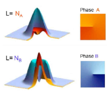
Figure 39: (Color online) Densities (left) and phases (right) in a two-component rotating Bose-Einstein condensate, as obtained from the Gross-Pitaevskii equations, for a ratio of atom numbers in the two components of $N_{A}/N_{B}=0.36$ and equal coupling strengths $g_{AA}=g_{AB}=g_{BB}=50$ a.u. (The densities are cut in one quadrant in order to visualize them for both components in one diagram). The rotational frequency is $\Omega=0.45$. The upper panel shows a coreless vortex at angular momentum $L=N_{A}$, where the smaller component $A$ shows a unit vortex at the center, as it is clearly seen from the phase of $\Psi_{A}$ plotted to the right (from dark to light shading), changing by $2\pi$ when the center is encircled once. The phase singularity is absent in $B$ component. The lower panel shows the case $L=N_{B}$, where now the larger component encircles the smaller one, filling the unit vortex at the center. The phase singularity consequently now occurs in the order parameter of $B$ component, as shown to the right (from dark to light blue). After data from Bargi et al. (2008).

At $L/N_{A}=1$, the system forms a single vortex in the smaller component $A$, which is clearly seen in the phase plot of the order parameter in Fig. 39. The phase jump is $2\pi$ along any closed path encircling the origin. The larger component rests at the origin $L_{B}=0$ with no vorticity (and, correspondingly, a flat phase profile in the order parameter). When the angular momentum reaches $L=N_{B}$, a singly-quantized coreless vortex is formed in the larger component $B$, while the component $A$ now is stationary at the origin.

Referring back to the work of Skyrme in the context of nuclear and high-energy physics Skyrme (1961, 1962) such coreless vortices were also called “skyrmions”, see the review by Kasamatsu et al. (2005a)..

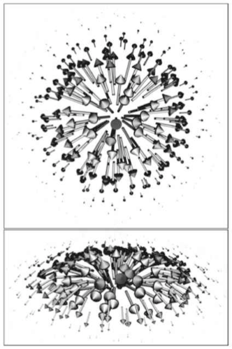
Figure 40: Schematic view of a skyrmion (top and perspective). The spin tilts from “up” for one component at the center, where one component shows a maximum density filling the vortex in the other component, to “down” towards the edge. From Mueller (2004).

A very graphic illustration of the pseudospin behavior in a single coreless vortex state is given in Fig. 40 Mueller (2004), showing the top and perspective view of such a skyrmion in a two-component system.

As $L$ increases, beyond $L=N_{B}$, a second vortex enters the larger component $B$, merging with the other vortex at $L=2N_{B}$. The smaller component $A$ remains localized at the center, and the system as a whole has a two-fold phase singularity at the center. An example is shown in Fig. 41. The central minimum in the density of the larger component $B$ expands with increasing angular momentum. It encircles the smaller one, that is non-rotating and localized at the trap center. A phase change of $4\pi$ in a closed path around the center indicates a vortex that is two-fold quantized. At $L=3N_{B}$ a triple phase singularity emerges at the center, but eventually the scenario breaks down with increasing rotation frequency.

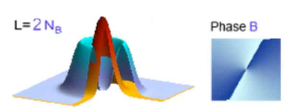
Figure 41: (Color online) Densities (left) and phases (right) of the Gross-Pitaevskii order parameters in a two-component rotating Bose-Einstein condensate with a coreless vortex with a double phase singularity. For notation see Fig. 39 above. After data from Bargi et al. (2008).

In single-component quantum liquids, multiply-quantized vortices are not favored in parabolic potentials. However, any external potential that grows more rapidly than quadratically may give rise to these giant vortex structures Lundh (2002); Kavoulakis and Baym (2003) discussed in Sec. IV.5 before. In two-component systems, it was found that the smaller, non-rotating component at the trap center may effectively act as an additional potential to the (harmonic) trap confinement, rendering the potential effectively anharmonic close to the trap center for the rotating component Bargi et al. (2007). With increasing rotation, both components carry a finite fraction of the total angular momentum, and multiply quantized or “giant” vortex states are no longer energetically favorable.

In exact diagonalization studies of multi-component systems, the additional degree of freedom through the pseudospin increases the dimension of the Hamiltonian matrix significantly, which leads to severe restrictions in the particle numbers or angular momenta that can be studied. Nevertheless, the results obtained for few-particle systems confirm the existence of Anderson-Toulouse and Mermin-Ho types of coreless vortices, as they were obtained within the Gross-Pitaevskii approach. For a two-component system with $N_{A}+N_{B}=8$ bosons with contact interactions in a harmonic trap, Fig. 42 shows the total angular momentum $L$ as a function of the rotational frequency $\Omega/\omega$. As in the case of scalar Bose gases (see Fig. 14 in Sect. IV.2 above), plateaus with increasing $\Omega$ can be associated with vortices that successively enter the bosonic cloud with increasing trap rotation Butts and Rokhsar (1999); Kavoulakis et al. (2000). These plateaus correspond to cusp states along the yrast line in the two-component system Bargi et al. (2010).

Figure 42: (Color online) Angular momentum as a function of the trap rotation frequency (in arbitrary units) for $N=8$ bosons with equal masses and interactions, in a harmonic trap, for equal population ($N_{A}=N_{B}=4$) (red line) and unequal population ($N_{A}=2$ and $N_{B}=6$) (green line). From Bargi et al. (2010).

The exact quantum states retain the symmetry of the Hamiltonian, and thus one must turn to conditional probability densities (pair-correlation functions) and reduced wave functions to map out the internal structure of the wave function, as discussed in Sec. II. For unequal populations of the two species, here $N_{A}=2$ and $N_{B}=6$, at those angular momenta where the pronounced plateaus occur in the $L$-versus-$\Omega$-plot in Fig. 42, the pair-correlations are shown in Fig. 43.

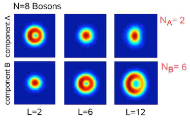
Figure 43: (Color online) Density plots of conditional probabilities for a two-component few-boson system in a harmonic trap, with two bosons in component $A$ and six bosons in component $B$. The reference point was chosen in component $B$ at an off-center position close to the maximum of the probability density. Axes are from $(-4,4)$ in atomic units. The color scale in the density plots is from blue (zero) to red (maximum). (To increase the visibility, the plot range of the conditional probablities in the two components was re-scaled to the same constant in all panels.) The charge deficiency of the vortex cores causes deep minima to appear in the pair-correlation functions. After Bargi et al. (2010).

At $L=2$ a vortex is seen as a hole at the center in the smaller component, encircling the larger component that forms a Gaussian at the trap center. At angular momentum $L=6$ a single vortex is created in the larger component, as seen in the middle panel. Twice this angular momentum creates a two-fold quantized vortex structure in the larger component. The existence of coreless vortices, as predicted by the Gross-Pitaevskii equation in the mean-field limit (Sec. V.2), is accurately reproduced by the exact solutions in the few-body regime.

V.2.2 Condensates with symmetric components

When the cloud has equal populations of the two components, i.e., $N_{A}=N_{B}$, a different scenario emerges: a vortex enters each of the components from “opposite” sides, reaching a minimum distance of one oscillator length from the center of the trap when $L=N_{A}=N_{B}$ Christensson et al. (2008a). An example is given by the Gross-Pitaevskii solution shown in the upper panel of Fig. 44.

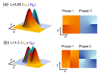
Figure 44: (Color online) Mean-field order parameters (left) and phases (right) of a symmetric condensate with $N_{A}=N_{B}$, at $L=1.2(N_{A}+N_{B})$, for equal coupling strengths $g_{AA}=g_{AB}=g_{BB}=50$, showing a) one and b) two interlaced coreless vortices in the two components. Component $B$ is only shown in a half-plane to make the vortex in the component $A$ visible. After data from Bargi et al. (2008).

Similarly to the one-component case, increasing rotation adds more vortices to the cloud. For two equal components, the vortices become interlaced, with density maxima in one component located at the vortices in the other, minimizing the interaction energy between the different components (lower panel of Fig. 44). In the limit of large $N$ and $L$ a lattice of coreless vortices is formed Kasamatsu et al. (2005a).

These Gross-Pitaevskii results are in good correspondence with exact diagonalization results of few-particle systems. The left panel of Figure 45 shows conditional probability densities of a symmetric configuration $N_{A}=N_{B}=4$. When $L$ equals $N_{A}=N_{B}=4$, the clouds separate, with a vortex hole emerging at the maximum density location in the other component. These solutions correspond to a Mermin-Ho vortex (or a meron pair, where each meron accounts for half of the spin texture of the coreless vortex) as obtained in Gross-Pitaevskii theory Kasamatsu et al. (2005a).

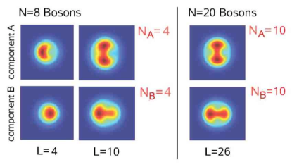
Figure 45: (Color online) As in Fig. 43, but for equal components, $N_{A}=N_{B}=4$ (left panel). The density minima in one component coincide with the density maxima in the other component. This suggests that these states are finite-size precursors of interlaced vortex lattices that occur in the limit of large $N$. The picture becomes much more clear for larger particle numbers, as shown in the right panel for $N=20$ and $L=26$. After Bargi et al. (2010).

For higher angular momenta, as here for $L=10$, the correlation functions indicate interlaced vortices as in Fig. 44 above, with density maxima in one component localizing at the minima (vortex cores) in the other component. The interlaced pattern of density minima and maxima becomes more apparent with higher particle number as shown in the right panel of Fig. 45 for $N=20$ bosons, where $N_{A}=N_{B}=10$, at angular momentum $L=26$.

The conditional probability densities average out the effect of phase singularities as signatures of vortices. However, the nodal structure of the many-body state may straightforwardly be probed by reduced wave functions Saarikoski et al. (2009) (see Sec. II.3.3), as shown in Fig. 46 for a system with $N_{A}=N_{B}=3$ bosons.

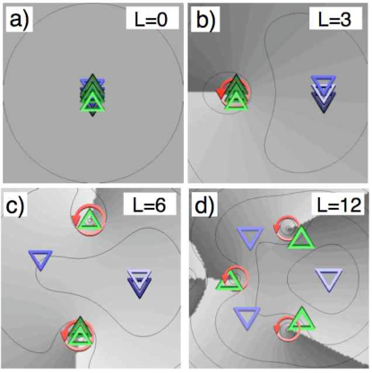
Figure 46: (Color online) Reduced wave functions in a symmetric system of $N_{A}=N_{B}=3$ bosons, showing the correlations between phase singularities (marked with circles) with the most probable positions of the particles of opposite species (marked with triangles). This is an indication for the formation of coreless vortices one-by-one in the system as the angular momentum increases. The figure shows a) the non-rotating state, b) a state with one coreless vortex per particle species, c) two coreless vortices, and d) three coreless vortices. Note that for identical components $A$ and $B$, the reduced wave functions for the two species are necessarily symmetric, and only one component is shown here. After Saarikoski et al. (2009).

Coreless vortices form one-by-one as the angular momentum increases: in the example shown here for $L=6$ and $L=12$, the phase singularities in one component occur at the most probable positions of the particles of the other component, indicating formation of two and three coreless vortices, respectively, in each particle component (Fig. 46).

V.2.3 Vortex lattices and vortex sheets

Vortex lattices in two-component bosonic condensates may show a variety of different structures, depending on the strength and sign of the interspecies interaction Mueller and Ho (2002). In the antiferromagnetic case ($c_{2}>0$), for weak interactions square lattices form, whereas for strong interactions the vortices are arranged into triangular Abrikosov lattices. In the former case the square lattice is energetically favoured because the antiferromagnetic interaction between adjacent vortex holes makes a triangular lattice frustrated Kasamatsu et al. (2003). At $c_{2}=0$ the system has metastable states such as a stripe phase. In the regime of ferromagnetic interspecies coupling ($c_{2}<0$), spin domains spontaneously form. These vortex sheets form “serpentine-like” structures that are nested into each other Kasamatsu et al. (2003); Kasamatsu and Tsubota (2009). A number of metastable lattice structures that were energetically almost degenerate have also been found in an antiferromagnetic spin-1 BEC Kita et al. (2002).

V.3 Two-component fermion droplets

Recent electronic structure studies of quantum dots with spin degrees of freedom predicted the formation of coreless vortices in fermion droplets analogously to the bosonic case Petkovic and Milovanovic (2007); Dai et al. (2007); Koskinen et al. (2007); Saarikoski et al. (2009). This comes as no suprise since analogies in the structure between fermion and boson states (Sec. II.6) are not limited to single-component systems, but an approximate mapping between two-component fermion and boson states can be constructed as well. In the following we discuss coreless vortices in fermion droplets and some of the consequences of the fermion-boson analogy with few-electron droplets as a particular example.

V.3.1 Coreless vortices with electrons

The angular momentum for a system with eight fermions with both balanced ($N_{A}=N_{B}=4$) and unbalanced ($N_{A}=2$, $N_{B}=6$) component sizes, is shown as a function of the trap rotation frequency in Figure 47. The staircase shape is strikingly similar to the bosonic counterpart (Fig. 42) with $L_{\rm boson}=L_{\rm fermion}-L_{\rm MDD}=L_{\rm fermion}-28$. In the fermion case with asymmetric components $N_{A}=2$ and $N_{B}=6$, the first pronounced plateaus appear at $L=L_{\rm MDD}+N_{A}=28+2$ and $L=L_{\rm MDD}+N_{B}=28+6$, which correspond to a coreless vortex in the $A$ and $B$ component, respectively. In the case of symmetric component occupations $N_{A}=N_{B}=4$ the first major plateau moves to $L=L_{\rm MDD}+4$ and the coreless vortex configuration is analogous to a meron pair Petkovic and Milovanovic (2007) in bosonic systems. The lengths of these plateaus indicate that coreless vortex states are very stable also in fermion systems.

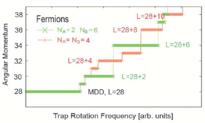
Figure 47: Angular momentum as a function of the trap rotation frequency (in arbitrary units) for $N=8$ fermions with symmetric (red) and asymmetric (green) component occupations, in Fig. 42 above. From Bargi et al. (2010).

The fermionic “quantum-dot” analog to the unbalanced few-boson system (with $N_{A}=2$ and $N_{B}=6$) discussed above would be a system with $N=8$ electrons and fixed $S_{z}=2$, which demands two spins antiparallel to the external magnetic field (component A) and six spins parallel to the field (component B). Both components form compact maximum density droplets independently at $L_{\rm MDD}=28$, that corresponds to the $L=0$ non-rotating condensate in the bosonic case. When the angular momentum exceeds that of the MDD by two units of $\hbar$, a hole forms at the center of the smaller component which is associated with a vortex state, while the larger one remains a MDD. This can be clearly seen from the pair-correlated density shown in Fig. 48. Note that in the case of fermions, there is a clearly visible exchange-correlation hole around the reference point in the pair-correlation. This is due to the Pauli principle which is naturally absent in the bosonic case. Due to the strong repulsion between the fermions, this hole is mirrored in the other component. For larger angular momentum, multiply quantized vortices are found in the larger component, in direct analogy to the bosonic case discussed above. This happens in our example for $L_{\rm fermion}=L_{\rm MDD}+6$ and $L_{\rm fermion}=L_{\rm MDD}+12$ (shown in Fig. 48).

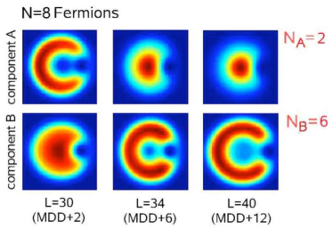
Figure 48: (Color online) Pair-correlated densities for fermions, as in Fig. 43, but here for fermions with Coulomb interactions ($N_{A}=2$ and $N_{B}=6$). Shown are angular momenta corresponding to the pronounced plateaus in Fig. 47. Compared to the bosonic case the densities show analogous structures except for an additional exchange hole at the reference point in component B which is reflected also in the component A due to Coulomb repulsion. From Bargi et al. (2010).

The case of equal components corresponds to fixed $S_{z}=0$. For $L=N_{A}=N_{B}$, just as in the bosonic case, a vortex appears at some distance from the trap center, with a density maximum on the other side, and vice-versa. These textures are again similar to the “meron” pairs in the bosonic two-component system discussed above. For higher angular momenta, the interlaced vortex lattice is seen for fermions at $L=L_{\rm MDD}+8$ and $L=L_{\rm MDD}+10$ (see Fig. 49). (Note again the occurrence of the exchange hole, that should not be confused with the holes of off-electron vortices.)

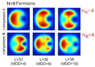
Figure 49: (Color online) Pair-correlated densities for fermions, as above, but for $S_{z}=0$, i.e., equal components ($N_{A}=4$ and $N_{B}=4$). From Bargi et al. (2010).

Figure 50 shows the reduced wave functions, see Eq. (11), for a two-component fermion droplet with Coulomb interactions and $N=6$ particles, with symmetric component occupations $N_{A}=N_{B}=3$. The sequence of states in this figure shows the formation of coreless vortices one-by-one inside the fermion droplet, in analogy to the bosonic case in Fig. 46 above, with the angular momenta for boson and fermion systems shifted by $L_{\rm fermion}=L_{\rm boson}+L_{\rm MDD}$. In comparison to the bosonic case, for fermions the Pauli vortices keep the particles further apart.

Figure 50: (Color online) Reduced wave functions in a two-component system. In a two-component fermion droplet with symmetric occupations $N_{A}=N_{B}=3$ the reduced wave function in the lowest Landau level reveals coreless vortices as correlations between phase singularities (circles) with the most probable positions of the particles of opposite spin (triangles). The figure shows a) the MDD state with total spin $S=3$ and $S_{z}=0$ b) a state with one coreless vortex per particle species c) two coreless vortices, and d) three coreless vortices. This sequence of states is analogous to that of a bosonic system in Fig. 46. Note that vortices of the MDD state are not shown in order to ease the comparison to the bosonic case. From Saarikoski et al. (2009).

V.3.2 Quantum dots with weak Zeeman coupling

The formation of coreless vortices, as discussed above, can be observed also in quantum dots where Zeeman coupling is weak. Then, the first reconstruction of the MDD may not be directly into the completely polarized states with one additional vortex, but into an excitation which is reminiscent of the vortex state, with one spin flipped anti-parallel to the magnetic field. This transition would be followed by a second one, involving a spin flip into the completely polarized state Oaknin et al. (1996). Siljamäki et al. (2002) studied the effect of Landau level mixing in the MDD reconstruction, using the variational quantum Monte Carlo method. They found significant changes in the ground states for systems consisting of up to 7 electrons. Figure 51 shows the different states of a 6-electron quantum dot in the vicinity of the MDD.

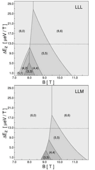
Figure 51: Partially polarized states beyond the maximum density droplet reconstruction, obtained from a variational Monte Carlo study by Siljamäki et al. (2002). The diagrams show the different states of a 6-electron quantum dot as a function of the magnetic field and the strength of the Zeeman coupling per spin in the lowest Landau level approximation (upper panel, LLL) and including Landau level mixing (lower panel, LLM). The states are labeled as ($N_{\uparrow},\Delta L$) where $N_{\uparrow}$ is the number of electrons with spins parallel to the magnetic field and $\Delta L=L-L_{\rm MDD}$ is the additional angular momentum with respect to the MDD. The Zeeman coupling strength for GaAs is marked by dashed lines. The confinement strength is $\hbar\omega=5$ meV and the material parameters are for GaAs, $m^{*}/m_{e}=0.067$ and $\epsilon_{r}=12.4$.

The partially polarized state after the MDD has a leading determinant of the form $|01111100\ldots\rangle$ for the majority spin component and $|100\ldots\rangle$ for the minority spin component: the vortex hole at the center of the dot in the majority spin component is filled by a particle with opposite spin polarization. Consequently, the state shows formation of a coreless vortex and is completely analogous to the case of asymmetric particle populations in a two-component bosonic systems, as discussed in Sec. V.2.1 above. The minority spin component has a MDD-like structure, which corresponds to the non-rotating component in the bosonic case, and the majority spin component shows a single vortex core localized at the center.

V.3.3 Non-polarized quantum Hall states

In the regime of rapid rotation vortices are expected to attach to particles also in two-component quantum droplets. One of the studied model wave functions for two-component states was introduced to explain the quantum Hall plateau at $\nu=2/3$ Halperin (1983)

$$\psi=\Pi_{i<j}^{N/2}(z_{i}-z_{j})^{q}\Pi_{k<l}^{N/2}(\tilde{z}_{k}-\tilde{z}_{l})^{q}\Pi_{m,n}^{N/2}(z_{m}-\tilde{z}_{n})^{p},$$ (51)

where $q$ is an odd integer (due to fermion antisymmetry), $p$ is a positive integer and the Gaussians have been omitted. The last product in Eq. (51) attaches $p$ vortices to each electron with opposite spin and these can be interpreted as coreless vortices. The corresponding nodal structure can also be found in spin-compensated few-electron systems near the $\nu=2/3$ filling. Figure 52 shows the reduced wave function of the $N_{A}=N_{B}=3,L=24$ electron state where one (Pauli) vortex is attached to each particle of the same spin and two (coreless) vortices are attached to particles of the opposite spin, in good agreement with the Halperin model with $q=1$ and $p=2$ Saarikoski et al. (2009). However, despite the correspondence in the nodal structures the overlap of this state with the Halperin wave function has been found to be small for large particle numbers, due to a mixing of spin states in the Halperin model Koskinen et al. (2007).

Figure 52: (Color online) Reduced wave function of the $L=24$ fermion state with symmetric occupations $N_{A}=N_{B}=3$. The nodal structure closely corresponds to that of the $q=2,p=1$ Halperin-wave function with one phase singularity in the component of the probing particle and two phase singularities in the opposite component. The approximate Landau level filling for the above finite size system is $\nu\approx 2/3$, just as for the Halperin state proposed to describe the $\nu=2/3$ quantum Hall plateau. The symbols in the figure were explained in Fig. 3 above. From Saarikoski et al. (2009).

V.4 Bose gases with higher spins

Experimentally, the investigations with two-component quantum gases have been extended to higher pseudospins ($T=1$) Leanhardt et al. (2003). For a rotating trap in the LLL approximation, the phase diagram of pseudospin $T=1$ bosons was studied by Reijnders et al. (2004), both using mean-field approaches and numerical diagonalization. The stability of the Mermin-Ho and Anderson-Toulouse vortices has been demonstrated for rotating ferromagnetic condensates with pseudospin $T=1$ Mizushima et al. (2002c, b). At small rotation the ground state is a coreless vortex. As an example, Fig. 53 shows the ground state structure of a ferromagnetic $T=1$ spinor condensate for the three different components of the order parameter Martikainen et al. (2002). The 3D trap was chosen with strong confinement in the $z$-direction of a harmonic trap, such that the system was effectively two-dimensional. The density distributions (where light color corresponds to the maximum density) in the $x-y$-plane are shown for $m=1,0,$ and $-1$. The $m=\pm 1$ components show two coreless vortices in much similarity to the two-component case discussed above. The third component, $m=0$, shows a regular array of four vortices that occur at the same positions of the coreless vortices.

Figure 53: Density plots of the Gross-Pitaevskii order parameters of the three components ($m=-1,0,1$) for a $T=1$ ferromagnetic condensate (see text). The calculation was performed for $1.7\times 10^{4}$ bosonic atoms of ⁸⁷Rb. Length units in the figure are in oscillator lengths. The total angular momentum per particle for the state shown was $L/N=1.85$, and the rotation frequency in units of the trap frequency was $\Omega=0.17$. White color indicates maximum density. After Martikainen et al. (2002).

VI Summary and Outlook

In finite systems with only a small number of particles, vortex formation can be studied by a numerical diagonalization of the many-body Hamiltonian. Often, a reasonable approximation is to assume the confinement to be a two-dimensional harmonic oscillator and to restrict the single-particle basis to the lowest Landau level. This is in particular the case in the limit of weak interactions. The close relationship of the many-body problem to the quantum Hall liquid then helps to explain the vortex localization and the similarity of vortex formation in boson and fermion systems. The many-body energy spectrum, although experimentally yet inaccessible, provides a wealth of information on the localization of vortices and their mutual interactions. The energy spectrum should also allow an approximation of the partition function and thus evaluation of temperature effects in future studies Dean and Papenbrock (2002).

The exact diagonalization is limited to systems with only a few particles. Mean-field and density-functional methods are necessary for capturing basic features of vortices in larger systems. In general, the density-functional methods describe the vortex structures in excellent qualitative agreement with the exact diagonalization results. In most density-functional approaches, the particles move in an effective field which allows internal symmetry breaking, making the observation of vortices more transparent than in the exact diagonalization method. However, the present state-of-the-art density-functional approaches fail to describe properly the highly-correlated regime at small filling fractions where vortices start to attach to particles, forming composites.

Experimentally, clear signatures of vortices in small electron droplets are still waiting to be observed. Imaging methods of electron densities in quantum dots may provide direct evidence of vortex formation in the future Fallahi et al. (2005); Dial et al. (2007); Pioda et al. (2004). The predicted localization of vortices in asymmetric confinements and in the presence of pinning impurities open a possible way to direct detection of vortices by means of measurements of the charge density of the electron droplet. Scanning probe imaging techniques have been developed to visualize the subsurface charge accumulation Tessmer et al. (1998), localized electron states Zhitenev et al. (2000) and charge flow Topinka et al. (2003) of a quantum Hall liquid. Similar methods could also turn out to be useful in probing electron density of two-dimensional electron droplets in quantum dots.

In rotating traps the present observation techniques are based on releasing the atoms from the trap and are limited to large atom numbers. Naturally, the experimental goal has been the study of large condensates. Optical lattices, with a small number of atoms in each lattice site, could in the future provide information of vortex formation in the few-body limit.

Despite experimental and theoretical advances in studies of rotating finite-size systems this review can provide only glimpses of this rich field of physics where vorticity plays a central role. Many important theoretical results presented here remain unverified in experiments. Theoretical challenges remain as well, especially in the regime of rapid rotation Baym (2005) where strong correlations may lead to emergence of exotic states. Vortex localization and ordering in the transition regime to a quantum Hall liquid, as well as the breakdown of this liquid state into a crystalline one, are still lively discussed themes in the field.

References

- Abo-Shaer et al. (2001) Abo-Shaer, J. R., C. Raman, J. M. Vogels, and W. Ketterle, 2001, Science 292, 476.
- Abrikosov (1957) Abrikosov, A. A., 1957, Zh. Eksperim. i Teor. Fiz. 32, 1442, [English translation in Soviet Phys. JETP 5, 1174 (1957)].
- Aifer et al. (1996) Aifer, E., B. Goldberg, and D. Broido, 1996, Phys. Rev. Lett. 76, 680.
- Andersen et al. (2003) Andersen, A., T. Bohr, B. Stenum, J. J. Rasmussen, and B. Lautrup, 2003, Phys. Rev. Lett. 91, 104502.
- Anderson et al. (1995) Anderson, M., J. Ensher, M. Matthews, C. Wieman, and S. Cornell, 1995, Science 269, 198.
- Anderson and Toulouse (1977) Anderson, P., and G. Toulouse, 1977, Phys. Rev. Lett. 38, 508.
- Andrei et al. (1991) Andrei, E., S. Yücel, and L. Menna, 1991, Phys. Rev. Lett. 26, 3704.
- Anisimovas et al. (2008) Anisimovas, E., M. B. Tavernier, and F. M. Peeters, 2008, Phys. Rev. B 77, 045327.
- Ashoori (1996) Ashoori, R., 1996, Nature 379, 413.
- Attaccalite et al. (2002) Attaccalite, C., S. Moroni, P. Gori-Giorgi, and G. Bachelet, 2002, Phys. Rev. Lett. 88, 256601.
- Attaccalite et al. (2003) Attaccalite, C., S. Moroni, P. Gori-Giorgi, and G. Bachelet, 2003, Phys. Rev. Lett. 91, 109902.
- Austing et al. (1999a) Austing, D. G., S. Sasaki, S. Tarucha, S. M. Reimann, M. Koskinen, and M. Manninen, 1999a, Phys. Rev. B 60, 11514.
- Austing et al. (1999b) Austing, G., Y. Tokura, T. Honda, S. Tarucha, M. Danoesastro, J. Janssen, T. Oosterkamp, and L. Kouwenhoven, 1999b, Jpn. J. Appl. Phys. 38, 372.
- Baardsen et al. (2009) Baardsen, G., E. Tölö, and A. Harju, 2009, Phys. Rev. B 80, 205308.
- Baelus et al. (2004) Baelus, B. J., L. R. E. Cabral, and F. M. Peeters, 2004, Phys. Rev. B 69, 064506.
- Baelus and Peeters (2002) Baelus, B. J., and F. M. Peeters, 2002, Phys. Rev. B 65, 104515.
- Baelus et al. (2001) Baelus, B. J., F. M. Peeters, and V. A. Schweigert, 2001, Phys. Rev. B 63, 144517.
- Barberán et al. (2006) Barberán, N., M. Lewenstein, K. Osterloh, and D. Dagnino, 2006, Phys. Rev. A 73, 063623.
- Bargi et al. (2007) Bargi, S., J. Christensson, G. M. Kavoulakis, and S. M. Reimann, 2007, Phys. Rev. Lett. 98, 130403.
- Bargi et al. (2010) Bargi, S., J. Christensson, H. Saarikoski, A. Harju, G. Kavoulakis, M. Manninen, and S. M. Reimann, 2010, Physica E 42, 411.
- Bargi et al. (2008) Bargi, S., K. Karkkainen, J. Christensson, G. Kavoulakis, M. Manninen, and S. Reimann, 2008, AIP Conf. Proceedings 995, 25.
- Barranco et al. (2006) Barranco, M., R. Guardiola, S. Hernández, R. Mayol, J. Navarro, and M. Pi, 2006, J. Low Temp. Phys. 142, 1.
- Barrett et al. (2001) Barrett, M., J. Sauer, and M. Chapman, 2001, Phys. Rev. Lett. 87, 010404.
- Barrett et al. (1995) Barrett, S., G. Dabbagh, L. Pfeiffer, K. West, and R. Tycko, 1995, Phys. Rev. Lett. 74, 5112.
- von Barth (1979) von Barth, U., 1979, Phys. Rev. A 20, 1693.
- Baym (2001) Baym, G., 2001, J. Phys. B: At. Mol. Opt. Phys. 34, 4541.
- Baym (2003) Baym, G., 2003, Phys. Rev. Lett. 91, 110402.
- Baym (2004) Baym, G., 2004, Phys. Rev. A 69, 043618.
- Baym (2005) Baym, G., 2005, J. Low Temp. Phys. 138.
- Baym and Pethick (1996) Baym, G., and C. Pethick, 1996, Phys. Rev. Lett. 76, 6.
- Baym and Pethick (2004) Baym, G., and C. Pethick, 2004, Phys. Rev. A 69, 043619.
- Baym et al. (1969) Baym, G., C. Pethick, and D. Pines, 1969, Nature 224, 673.
- Bedanov and Peeters (1994) Bedanov, V. M., and F. M. Peeters, 1994, Phys. Rev. B 49(4), 2667.