June 2010

Direct and Indirect Detection of Neutralino Dark
Matter and Collider Signatures in an $SO(10)$ Model
with Two Intermediate Scales

Manuel Drees${}^{a\,}$, Ju Min Kim${}^{a\,}$, and Eun-Kyung Park${}^{a,b\,}$

^aPhysikalisches Institut and Bethe Center for Theoretical Physics, Universität Bonn, Nussallee 12, 53115 Bonn, Germany
^bLAPTH, Université de Savoie, CNRS,
B.P. 110, F-74941 Annecy-le-Vieux Cedex, France

1 Introduction

Grand Unified Theories (GUTs) based on the gauge group $SO(10)$ have been considered good candidates for the unification of electroweak and strong interactions [1]. All matter fields of one generation are incorporated in a single irreducible representation, the spinor 16. Moreover, the “seesaw” mechanism [2], which can explain small neutrino masses as indicated by neutrino oscillations, is naturally embedded.

In [3], two of us in particular chose a model by Aulakh et al. [4], a supersymmetric $SO(10)$ model with two intermediate scales: $SO(10)$ is first broken to $SU(4)_{C}\times SU(2)_{L}\times SU(2)_{R}$ by a 54 dimensional Higgs at the GUT scale $M_{X}$; then to $SU(3)_{C}\times U(1)_{B-L}\times SU(2)_{L}\times SU(2)_{R}$ by 45 at scale $M_{C}$; finally to the Standard Model gauge group by ${\bf 126}+{\bf\overline{126}}$ at scale $M_{R}$. Imposing the unification condition for the gauge couplings fixes the intermediate scales $M_{C}$ and $M_{R}$ for given $M_{X}$; i.e. $M_{X}$ is a free parameter. However, its lower bound is set by the lower bound on the lifetime of the proton [5]. We took $M_{X}=3\cdot 10^{15}$GeV as default value. In addition, a second pair of Higgs doublets was introduced, in order to modify the minimal $SO(10)$ predictions for the masses of quarks and leptons, which are not consistent with experiments. In order to compare the low energy phenomenology of the model with that of mSUGRA [6], we assumed universal soft breaking parameters ($m_{0},M_{1/2},A_{0}$) as boundary condition at the GUT scale.

The 126–dimensional Higgs whose vacuum expectation value breaks $SU(2)_{R}\times U(1)_{B-L}$ to $U(1)_{Y}$ also gives Majorana masses to the right–handed neutrinos. The resulting masses for the light neutrinos are schematically written as

$$m_{\nu}=\frac{m_{D}^{2}}{M_{N}}=\frac{(Y_{\nu}\langle H_{u}^{0}\rangle)^{2}}{Y_{N}\langle{\bf\overline{126}}\rangle}.$$ (1)

The Yukawa coupling $Y_{N}$, and to a lesser extent $Y_{\nu}$, gives new contributions to the Renormalization Group Equations (RGEs) of the MSSM Yukawa couplings and soft breaking parameters. Therefore the weak–scale masses, and thus the radiative electroweak symmetry breaking and the relic density of Dark Matter, depend on $Y_{N}$, and hence on the light neutrino masses for fixed $M_{R}$. This remains qualitatively true for other $SO(10)$ GUTs with a “type–I” seesaw mechanism at an intermediate scale. Note that $Y_{\nu}$ unifies with the up–type quark Yukawa couplings, and is hence fixed. For given $M_{R}$, and hence given $\langle{\bf\overline{126}}\rangle$, the absolute scale of the light neutrino masses is thus determined by $Y_{N}$, with larger $Y_{N}$ yielding lighter neutrinos. For our minimal choice $M_{X}=3\cdot 10^{15}$ GeV, the requirement that $Y_{N}$ remains perturbative at least up to scale $M_{X}$ therefore leads to the lower bound $m_{\nu}\raisebox{-3.69899pt}{~{}\shortstack{$>$ \\ [-0.07cm] $\sim$}}~{}0.15$ eV on the mass of the heaviest light neutrino.

For our current study the most important modification of the weak–scale spectrum is the reduction of the higgsino mass parameter $|\mu|$, which comes about as follows. The weak–scale stop masses are reduced compared to the mSUGRA prediction, due to the Yukawa coupling given by [3]

$$W_{\rm Yuk,422}\ni\frac{1}{2}Y_{N}\left(F^{c}\overline{\Sigma}_{R}F^{c}+F\overline{\Sigma}_{L}F\right)\,.$$ (2)

Here $W_{\rm Yuk,422}$ is the superpotential valid between the scales $M_{C}$ and $M_{X}$, $\overline{\Sigma}_{R}$ and $\overline{\Sigma}_{L}$ are in the (${\bf 10},{\bf 1,3}$) and ($\overline{\bf 10},{\bf 3,1}$) representation, respectively, of the gauge group $SU(4)_{C}\times SU(2)_{L}\times SU(2)_{R}$, and $F$ and $F^{c}$ denote quark and lepton superfields in the (4,2,1) and ($\overline{\bf 4},{\bf 1,2}$) representation. This reduces the term $\propto Y_{t}^{2}$ in the RGE for $m_{H_{u}}^{2}$, leading to an increase of $m_{H_{u}}^{2}$ at the weak scale. As a result, electroweak symmetry breaking requires smaller values $|\mu|$ than in mSUGRA.

Another distinctive feature of the model is the rapid increase of the gauge couplings at high energies. This is due to the introduction of large additional Higgs representations, needed in order to break the gauge symmetry. As a result, relations between weak–scale and the GUT–scale soft breaking parameters are modified [3]. In particular, for a given universal gaugino mass $M_{1/2}$ at the GUT scale, the $SO(10)$ model predicts much smaller gaugino masses at the weak scale than mSUGRA does.

In ref.[3] it was shown that thermal neutralino Dark Matter remains viable, although the allowed region of parameter space is even more highly constrained than in mSUGRA. In the next Section, we will focus on the detectability of this Dark Matter candidate by direct and indirect searches. In Sec. 3, we compare signatures at the LHC between mSUGRA and this $SO(10)$ model for two benchmark points. Finally, we conclude in Sec. 4.

2 Direct and indirect detection of Dark Matter

All results presented in this Section are obtained using a modified version [3] of SOFTSUSY 2.0 [7] to evaluate the mass spectra at the weak scale. These are then fed into micrOMEGAs 2.2 [8] to calculate the LSP relic density. If this is found acceptable, we feed the same low–energy spectrum into DarkSUSY 5.0.2 [9] for the calculation of various Dark Matter detection rates [10].

Specifically, we compute: elastic LSP–proton scattering cross sections due to spin–independent as well as spin–dependent interactions; the muon flux resulting from LSP annihilation in the Sun; and the antiproton flux from LSP annihilation in the halo of our galaxy. In all cases we compare with the sensitivities of the best current and/or near–future experiments. In most cases, we only consider parameter sets leading to a relic density within two standard deviations of the value found by combining WMAP data with other cosmological observations [11]:

$$\Omega_{CDM}h^{2}=0.1131\pm 0.0068\ \ (2\sigma\ {\rm range}).$$ (3)

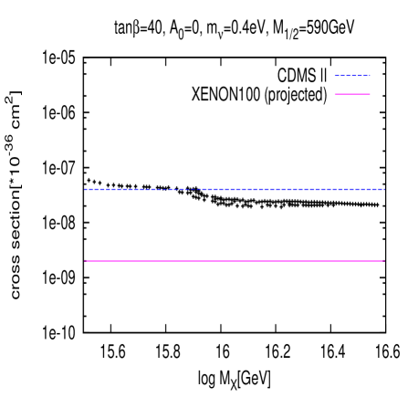
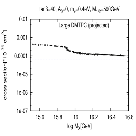
Figure 1: The $M_{X}$ dependence of the SI (left frame) and SD (right frame) neutralino–proton scattering cross section. $m_{0}$ is varied such that the relic density satisfies the constraint (3). The neutralino mass $m_{\chi}=124$ GeV, for $M_{X}=10^{15.5}$ GeV, increases to $235$ GeV for $M_{X}=10^{16.6}$ GeV. The experimental constraints are taken for $m_{\tilde{\chi}_{1}^{0}}=120$ GeV.

We begin our discussion by analyzing the impact of reducing $M_{X}$, i.e. “switching on” the intermediate scales, on the elastic LSP–proton scattering cross section. Figure 1 shows the spin–independent (SI; left frame) and spin–dependent (SD; right frame) contributions to this cross sections as we vary $M_{X}$ while most soft breaking parameters as well as the light neutrino masses are kept fixed. The scalar mass $m_{0}$ is varied along with $M_{X}$ such that the relic density lies in the range of Eq.(3). Note that $m_{0}^{2}\gg M^{2}_{1/2}$ in this plot, i.e. we are in the region of significant higgsino–neutralino mixing, which is most favorable for direct neutralino Dark Matter searches. As a result, the spin–independent cross section is always well above the projected sensitivity of the XENON100 experiment [12], while the spin–dependent cross section lies above the projected sensitivity of the DMTPC experiment [12].

While these gross features remain unchanged, we see that, as $M_{X}$ decreases, i.e. as the deviation from mSUGRA becomes larger, the cross section is enhanced, so that for the lowest $M_{X}$, the spin–independent cross section slightly exceeds the limit set by the CDMS II experiment [13]. This is mostly due to the reduction of the LSP mass for fixed $M_{1/2}$ in the model with intermediate scales, which we mentioned near the end of Sec. 1. In particular, for $M_{X}\leq 8\cdot 10^{15}$ GeV, $m_{\tilde{\chi}_{1}^{0}}<m_{t}$, so that $\tilde{\chi}_{1}^{0}\tilde{\chi}_{1}^{0}\rightarrow t\bar{t}$ annihilation is forbidden. The loss of this important annihilation channel has to be compensated by increasing bino–higgsino mixing, i.e. by decreasing $\mu$, which in turn is accomplished by increasing $m_{0}$. This leads to increased couplings of the lightest neutralino to neutral Higgs bosons as well as to the $Z^{0}$ boson. Note that in scenarios with gaugino mass unification, first generation squarks are always much heavier than the lightest neutralino, suppressing their contributions to LSP–nucleon scattering. Choosing $m_{0}^{2}\gg M_{1/2}^{2}$, as done here, further strengthens this hierarchy, so that Higgs and $Z^{0}$ exchange contributions largely determine the SI and SD cross sections, respectively.

The curves in Figs. 1 show a noticeable negative slope even away from this threshold. In case of the SI cross section, this is due to the reduction of the mass of the heavier neutral CP–even Higgs boson with decreasing $M_{X}$, which goes along with the reduction of the weak–scale gaugino masses (although for fixed $m_{0}$ the ratio $m_{A}/m_{\tilde{\chi}_{1}^{0}}$ slightly increases with decreasing $M_{X}$ [3]). Note also that decreasing $m_{\tilde{\chi}_{1}^{0}}$ requires a simultaneous, if slower, decrease of $\mu$, since otherwise the higgsino–component of $\tilde{\chi}_{1}^{0}$ would become too small, yielding too small an annihilation cross section. This decrease of both weak–scale gaugino masses and of $\mu$ with decreasing $M_{X}$ implies that the higgsino components of the LSP become more different in magnitude; note that they become identical in size for $|\mu|\gg M_{Z}$. This in turn enhances the $\tilde{\chi}_{1}^{0}\tilde{\chi}_{1}^{0}Z^{0}$ coupling, which is proportional to the difference of the squares of these components [6].

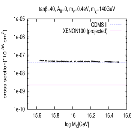
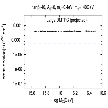
Figure 2: As Fig. 1, except that $M_{1/2}$ has also been varied along with $M_{X}$, such that the mass of the lightest neutralino is kept fixed at 140 GeV.

Figs. 2 show results analogous to those in Fig. 1, except that now the gaugino mass parameter $M_{1/2}$ has been varied along with $M_{X}$ such that the LSP mass is kept fixed. This required taking larger values of $M_{1/2}$ for smaller $M_{X}$. As expected from our previous discussion, the effect of reducing $M_{X}$ is now quite small. The spin–independent cross section (left frame) increases by $\sim 20$% as $M_{X}$ is reduced to its minimal value. This can be explained as follows. Since now $m_{\tilde{\chi}_{1}^{0}}$ is kept fixed, we also have to keep $\mu$ essentially fixed in order to maintain the correct relic density. This requires reducing $m_{0}$ when $M_{X}$ is reduced. This in turn leads to a reduction of $m_{A}$, which over–compensates the increase of $m_{A}$ that would result if $M_{X}$ were reduced for fixed $m_{0}$ and fixed LSP mass. This implies a similar reduction for the mass of the heavier CP–even neutral Higgs boson whose exchange plays a prominent role in this cross section. However, it is not clear whether this variation is significant given astrophysical and likely experimental uncertainties. The variation of the spin–dependent cross section is even smaller.

Figs. 3 shows the same cross sections for smaller (heaviest) neutrino mass, $m_{\nu}=0.2$ eV, as well as larger gaugino mass, $M_{1/2}=1$ TeV. Recall that the smaller $m_{\nu}$ requires a larger Yukawa coupling $Y_{N}$, which, among other things, reduces the weak–scale $\tilde{\tau}$ masses. This allows to satisfy the relic density constraint (3) for two distinct choices of $m_{0}$. We continue to call the choice with $m_{0}^{2}\gg M_{1/2}^{2}$, and resulting sizable higgsino component of the LSP, the “focus point” [14], even though the $SO(10)$ model does not show “focusing” behavior of any Higgs soft breaking mass [3]. In the “co-annihilation” region the relic density is largely determined by $\tilde{\chi}_{1}^{0}-\tilde{\tau}_{1}$ co–annihilation [15] in both mSUGRA and the $SO(10)$ model.

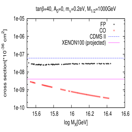
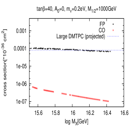
Figure 3: Dependence of the SI (left frame) and SD (right frame) neutralino–proton scattering cross section on $M_{X}$, for $m_{\nu}=0.2$ eV. We chose two points that represent the “focus point” (“FP”) region (black) and the “co–annihilation” (“CO”) region (red or grey). The neutralino mass varies between 220 GeV and 390 GeV at the smallest and largest $M_{X}$, respectively. The experimental constrains are taken for $m_{\tilde{\chi}_{1}^{0}}=220$ GeV, and scale essentially like $m_{\tilde{\chi}_{1}^{0}}$.

For the focus point, we find the SI cross section to be almost independent of $M_{X}$. Note that $m_{\tilde{\chi}_{1}^{0}}$ is now well above $m_{t}$ in the entire range of $M_{X}$ shown. Moreover, $m_{A}$ increases with decreasing $m_{\nu}$ [3]; the decrease of $m_{A}$ with decreasing $M_{X}$ is therefore less pronounced than in Fig. 1. Finally, reducing the LSP mass increases the annihilation cross section, which scales like $m_{\tilde{\chi}_{1}^{0}}^{-2}$ away from thresholds. In compensation, gaugino–higgsino mixing has to be reduced. This reduces the LSP couplings to neutral Higgs bosons, offsetting the effect of the reduction of $m_{A}$ as far as the SI cross section is concerned. In the SD case, we again observe a slight increase of the cross section with decreasing $M_{X}$, as in Fig. 1, away from the $t\bar{t}$ threshold. Note also that, in spite of the increased LSP mass, the “focus point” scenario remains easily testable by near–future direct search experiments, at least via the SI cross section.

On the other hand, for the co–annihilation point, both the SI and SD cross sections increase by one order of magnitude when $M_{X}$ is reduced to its smallest allowed value. Here the Dark Matter relic density is mainly determined by the mass difference between the LSP and the lightest stau, which does not strongly depend on $\mu$. Instead, the correct relic density is obtained through the direct effect of $m_{0}$ on $m_{\tilde{\tau}_{1}}$. Due to the strong (exponential) dependence of the relic density on the $\tilde{\chi}_{1}^{0}-\tilde{\tau}_{1}$ mass splitting, only relatively minor adjustments of $m_{0}$ are required, which do not lead to significant changes of $\mu$. In contrast, the additional Yukawa couplings in the $SO(10)$ model reduce $|\mu|$ all over the parameter space. Therefore, in the co–annihilation region the larger higgsino component of $\tilde{\chi}_{1}^{0}$ gives rise to larger scattering amplitudes, in particular via the Higgs– and $Z^{0}-$exchange diagrams that dominate the SI and SD cross sections, respectively. The SI cross section is enhanced in addition by the decreasing $m_{A}$. As a result, at the smallest value of $M_{X}$ this cross section even approaches the XENON100 sensitivity.

In order to understand the strong dependence of these cross sections on $M_{X}$, one has to keep in mind that reducing $M_{X}$ increases the effect of the new Yukawa coupling $Y_{N}$ in two ways. First, reducing $M_{X}$ reduces the intermediate scales $M_{R}$ and $M_{C}$ even more, i.e. $\ln(M_{X}/M_{C})$ and $\ln(M_{X}/M_{R})$ increase when $M_{X}$ is decreased. This increases the energy range where this coupling is effective in the RGE. Secondly, the reduction in $M_{R}$ has to be compensated by the increase of $Y_{N}$ in order to keep the very large Majorana neutrino mass in the see–saw expression (1) constant.

The most robust indirect neutralino Dark Matter detection signal [10] is due to the capture of DM particles by the Sun, which greatly enhances the neutralino density near the center of the Sun. Eventually capture and annihilation of neutralinos in the Sun reach equilibrium. The only annihilation products that can escape the Sun are neutrinos. In particular, muon neutrinos produce muons via charged current interactions; these muons can be searched for by “neutrino telescopes”.

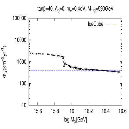
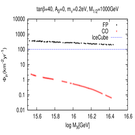
Figure 4: Neutrino–induced muon flux from neutralino annihilation in the Sun as a function of $M_{X}$ for $m_{\nu}=0.4$ eV (left); $m_{\nu}=0.2$ eV (right). The IceCUBE sensitivity limits are for the smallest LSP mass in the respective frames; in the relevant range of masses, the sensitivity limit scales roughly $\propto 1/m_{\tilde{\chi}_{1}^{0}}$.

In Figs. 4 we plot the resulting muon flux as function of $M_{X}$, and compare it to the “best case” sensitivity of IceCUBE [16], using the input parameters of Fig. 1 (left frame) and Fig. 3 (right). Note that the overall neutrino flux is essentially fixed by the capture rate. The neutralinos interact with nuclei in the Sun mostly via Higgs and $Z^{0}$ exchange. The capture rate is thus again sensitive to the higgsino components of the mostly bino–like neutralinos. It also depends on the mass of the neutralinos: the heavier the LSP, the less likely it is to lose enough energy in the interaction to become gravitationally bound to the Sun. The predicted muon flux therefore increases faster with decreasing $M_{X}$ than the cross sections shown in Figs. 1 and 3 do.

The muon flux also depends on the (mean) neutrino energy, since the neutrino charged current cross section increases with energy. Annihilation into pairs of $W^{\pm}$ or $Z^{0}$ bosons leads to the hardest neutrino spectra, and hence to the largest signals. Annihilation into $t\bar{t}$ gives a somewhat softer spectrum, since some of the energy is taken away by the $b-$quarks. This enhances the effect of the $t\bar{t}$ threshold visible in the left frame: To the left of this threshold, neutralinos predominantly annihilate directly into massive gauge bosons, while to the right of the threshold, annihilation into $t\bar{t}$ dominates.

Of course, the neutrino energy also scales with the mass of the annihilating neutralinos. Indeed, the sensitivity limit on the muon flux decreases with increasing LSP mass for $m_{\tilde{\chi}_{1}^{0}}\raisebox{-3.69899pt}{~{}\shortstack{$<$ \\ [-0.07cm] $\sim$}}~{}500$ GeV [16]. However, in the muon flux itself this effect is compensated by the reduction of the neutralino flux impinging on the Sun, which scales like $1/m_{\tilde{\chi}_{1}^{0}}$. Nevertheless, this effect keeps the expected flux in the “focus point” region well above the sensitivity limit even for the larger value of $M_{1/2}$ chosen in the right frame. However, the flux in the co–annihilation region remains well below the IceCUBE sensitivity even for the smallest possible value of $M_{X}$.

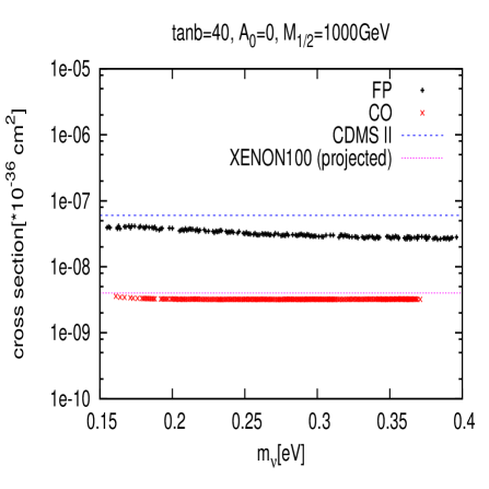
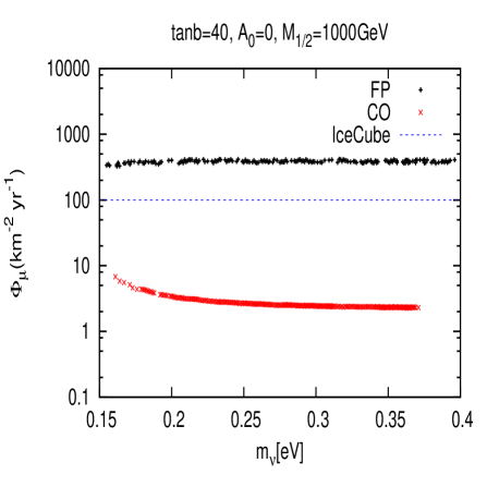
Figure 5: SI neutralino–proton scattering cross section (left) and neutrino–induced muon flux from neutralino annihilation in the Sun (right), as function of $m_{\nu}$.

In Fig. 5, we show the SI proton–neutralino cross section as well as the neutrino–induced muon flux as function of $m_{\nu}$, for $M_{X}=3\cdot 10^{15}$ GeV. We see that in the FP region, the cross section slightly increases with decreasing $m_{\nu}$. Recall that decreasing $m_{\nu}$, i.e. increasing the coupling $Y_{N}$, reduces $\mu$. In order to keep the relic density fixed one has to increase $\mu$ again by decreasing $m_{0}$, which in turn leads to the decrease of the Higgs boson masses; this overcompensates the increase of $m_{A}$ with decreasing $m_{\nu}$ if all soft breaking parameters are kept fixed. The reduced Higgs boson masses increase the scattering cross section. However, it also increases the importance of the $A-$exchange contribution to the $\tilde{\chi}_{1}^{0}$ annihilation cross section at rest. For $\tan\beta\gg 1$, $A-$exchange mostly leads to $b\bar{b}$ final states, which produce very soft neutrinos. This effect over–compensates the (small) increase in the neutralino capture cross section, leading to the (very slight) decrease of the muon flux with decreasing $m_{\nu}$ in the FP region.

In the co–annihilation region, increasing the Yukawa coupling $Y_{N}$ reduces $m_{\tilde{\tau}_{R}}$ as well as $\mu$. The two effects tend to cancel, but a net reduction of $m_{\tilde{\tau}_{1}}$ results. This has to be compensated by increasing $m_{0}$ in order to keep the relic density in the desired range. This, as well as the effect of $Y_{N}$ in the RGE, increases $m_{A}$. The increase of $m_{A}$ and the decrease of $\mu$ essentially cancel in the SI cross section. However, increasing $m_{A}$ also reduces the importance of neutralino annihilation to $b\bar{b}$. This increases the average neutrino energy, which explains the slight increase of the muon flux with decreasing $m_{\nu}$.

We have also computed the near–Earth flux of antiprotons due to the annihilation of relic neutralinos in the halo of our galaxy. As well known, the flux depends sensitively on several poorly known astrophysical quantities. One of these is the density of Dark Matter, which is reasonably well known “locally”, but not near the center of the galaxy, where it is largest. Note that, unlike positrons, antiprotons can diffuse from the galactic center to Earth. We illustrate this uncertainty by comparing three different halo models. The “N03” profile has been derived [17] starting from a profile extrapolated from $N-$body simulations [18], assuming that baryon infall compresses the Dark Matter distribution near the galactic center adiabatically. In the opposite extreme, one can assume that baryon infall heats the dark halo, leading [17] to a profile similar to the (phenomenologically apparently quite successful) “Burkert” profile [19]. Finally, the “NFW” profile [20] lies between these extremes.

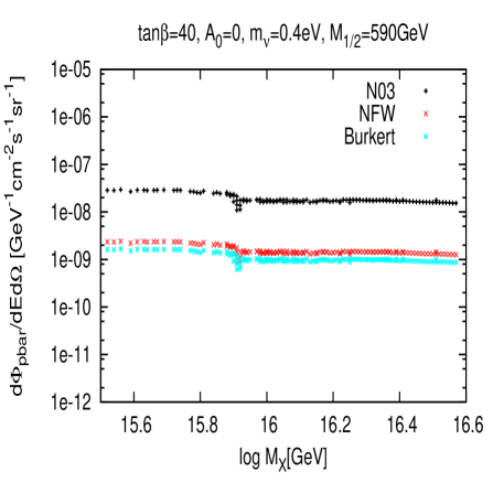
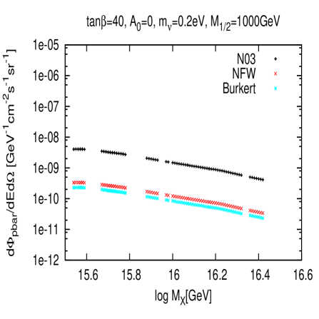
Figure 6: Antiproton differential flux for different halo models for $m_{\nu}=0.4$ eV (“focus-point”, left) and $m_{\nu}=0.2$ eV (“co-annihilation”, right).

Figs. 6 show the dependence of the antiproton flux on $M_{X}$. Antiprotons are produced in the Galactic halo due to the hadronization of antiquarks produced in neutralino Dark Matter annihilation. As a result, the typical $\bar{p}$ energy is well below $m_{\tilde{\chi}_{1}^{0}}$. We show their differential flux at a kinetic energy 20 GeV, where the signal–to–background ratio is expected to be optimal [21]. We illustrate the dependence on the halo model using the three profiles discussed above.

The left frame of Fig. 6 is for the “focus point” region, with small $Y_{N}$ and relatively small $M_{1/2}$. In this case the relic density is determined by $\tilde{\chi}_{1}^{0}$ annihilation with itself, and is dominated by annihilation from the $S-$wave, which is the only contribution relevant for the $\bar{p}$ flux. As a result, the $\tilde{\chi}_{1}^{0}$ annihilation cross section remains essentially constant in the left frame. However, we saw in Fig. 1, where the same parameters were used, that $m_{\tilde{\chi}_{1}^{0}}$ decreases by nearly a factor of two as $M_{X}$ is decreased. This increases the $\tilde{\chi}_{1}^{0}$ annihilation rate, computed as the product of flux and cross section, by almost a factor of four. However, decreasing $m_{\tilde{\chi}_{1}^{0}}$ also makes it increasingly more difficult to produce antiprotons at 20 GeV. As a result, the $\bar{p}$ flux near Earth only increases very slightly as $M_{X}$ is decreased.

The right frame shows results for a point in the co–annihilation region, with larger $M_{1/2}$ and smaller $m_{\nu}$. Here the relic density is essentially determined by $\tilde{\tau}_{1}-\tilde{\chi}_{1}^{0}$ co–annihilation. The annihilation cross section increases significantly with decreasing $M_{X}$, due to the decrease of (almost) all weak–scale sparticle and Higgs boson masses. Moreover, $m_{\tilde{\chi}_{1}^{0}}$ now remains so high that getting 20 GeV antiprotons is not difficult. As a result, the rate increases by about an order of magnitude as $M_{X}$ is reduced to its lower bound.

This seems impressive, but is still smaller than the difference in the predictions based on the N03 and Burkert profiles. Additional systematic uncertainties come from the propagation of the antiprotons; here we have used DarkSUSY default parameters. Note finally that the $\bar{p}$ flux that can be inferred from the $\bar{p}/p$ ratio measured by the PAMELA satellite [22] and the well–known [5] proton flux is about $2\cdot 10^{-7}$ GeV^-1cm^-2s^-1sr^-1, well above even the most optimistic prediction in Fig. 6. Given that the prediction for the background also has sizable uncertainties, we conclude that the observation of cosmic antiprotons is not a very promising test of the models discussed here.

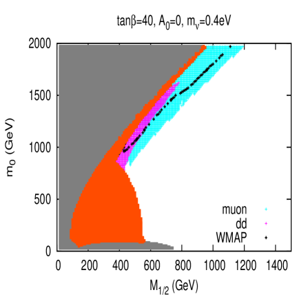
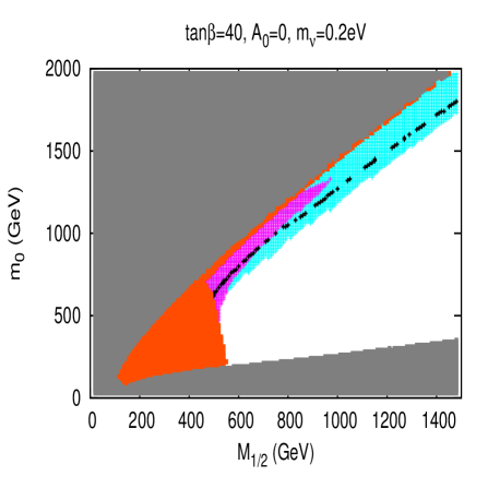
Figure 7: Regions in the $(M_{1/2},m_{0})$ plane for $m_{\nu}=0.4$ eV (left); $m_{\nu}=0.2$ eV (right). The grey area is excluded by the EWSB condition or by too light sfermions, and the scarlet area is excluded by the LEP limits on Higgs and chargino masses. The black points give us the correct Dark Matter relic density. The light blue region can be tested by searching for muon neutrinos originating from $\tilde{\chi}_{1}^{0}$ annihilation in the Sun, while in the magenta region, the $\tilde{\chi}_{1}^{0}p$ scattering cross section exceeds the CDMS–II bound. The dependence of the detectability on the WIMP mass is taken into account, but we assume a fixed local WIMP density.

Prospects for direct and indirect DM search in the $SO(10)$ model with the smallest allowed $M_{X}$ are summarized in Figs. 7, for two different values of $m_{\nu}$. The regions of parameter space that give the neutrino–induced muon flux from $\tilde{\chi}_{1}^{0}$ annihilation in the Sun above the IceCUBE sensitivity limit are depicted as light blue. The regions where the spin–independent neutralino–proton cross section exceeds the CDMS–II bound are shown in magenta. Note that we always assume fixed local neutralino density when deriving these bounds, independent of the value of $\Omega_{\tilde{\chi}_{1}^{0}}h^{2}$ predicted in standard cosmology. We also show the region excluded by the electroweak symmetry breaking (EWSB) condition or by too light sfermions (grey) as well as that excluded by the LEP limits [5] on the masses of Higgs bosons and charginos (scarlet). The black points are where the Dark Matter relic density satisfies Eq.(3).

We find that, as in mSUGRA [23], the region of high $m_{0}$, where $\tilde{\chi}_{1}^{0}$ has a sizable higgsino component, will soon be covered by direct searches and also by the neutrino indirect search. Recall from Figs. 5 that the region of parameter space to be probed by XENON100 is much larger than that probed by IceCUBE. Compared to mSUGRA, for given $M_{1/2},\ A_{0}$ and $\tan\beta$ this region occurs at significantly lower values of $m_{0}$; this is true in particular for small $m_{\nu}$, i.e. sizable Yukawa coupling $Y_{N}$ (right frame). Moreover, in this region neutralino Dark Matter remains detectable out to much larger values of $M_{1/2}$ than in mSUGRA, since the ratio $m_{\tilde{\chi}_{1}^{0}}/M_{1/2}$ is nearly two times smaller in our scenario than in mSUGRA.

The co–annihilation region is difficult to see in Figs. 7, since it is very narrow. It extends to $M_{1/2}\simeq 750\ (1400)$ GeV for $m_{\nu}=0.4\ (0.2)$ eV. Unfortunately this region will not be tested by near–future Dark Matter search experiments. However, we saw in Fig. 3 that the $\tilde{\chi}_{1}^{0}p$ scattering cross section exceeds that in mSUGRA by about an order of magnitude. Much of this region will therefore be testable by ton–scale direct Dark Matter detection experiments.

3 Collider searches

In this section, we consider signatures at the LHC for our model. It remains sufficiently similar to mSUGRA that the overall search prospects, i.e. the reach in sparticle masses, is essentially the same in both models; i.e., discovery should be possible out to $m_{\tilde{g}}\sim 3\ (2)$ TeV for $m_{\tilde{q}}\simeq\ (\gg)m_{\tilde{g}}$ [24], once the LHC reaches its full energy and luminosity. Of course, at the smallest allowed value of $M_{X}$ the reach in $M_{1/2}$ is nearly two times larger in our model, but $M_{1/2}$ is not measurable by TeV–scale experiments. We will therefore focus on ways to distinguish the model from mSUGRA using measurements at colliders, with emphasis on the LHC.

3.1 Benchmark points

We performed detailed analyses of collider signals for two distinct benchmark points. The input parameters as well as superparticle and Higgs spectra are listed in Table 1. We chose points that satisfy all constraints, including the Dark Matter relic density constraint (but ignoring the indication of a deviation of the magnetic dipole moment of the muon from the Standard Model prediction [25]). We chose $M_{X}$ at its lower bound of $3\cdot 10^{15}$ GeV, and small $m_{\nu}=0.2$ eV, in order to maximize the differences between our model and mSUGRA. On the other hand, we chose the parameters of the mSUGRA points such that the sparticle spectra are as similar as possible to those of the corresponding $SO(10)$ benchmark points. In particular, we adjust the values of $M_{1/2}$ such that the gluino masses are essentially the same in both models. Moreover, we chose the same $m_{0}$ in both models, since this gives similar first and second generation squark masses. In this way we hope to isolate the non–trivial effects of the additional couplings via the RGE.

parameter	$SO(10)$ 1	mSUGRA 1	$SO(10)$ 2	mSUGRA 2a	mSUGRA 2b
$M_{1/2}$	1100	600	1000	550	550
$m_{0}$	1400	1400	280	280	280
$A_{0}$	0	300	0	-120	0
$\tan\beta$	40	52	40	40	41.5
$\mu$	307	587	607	682	663
$\tilde{\chi}^{0}_{1}$	243	253	229	227	227
$\tilde{\chi}^{0}_{2}$	313	468	430	431	430
$\tilde{\chi}^{0}_{3}$	317	597	615	690	671
$\tilde{\chi}^{0}_{4}$	519	618	628	698	680
$\tilde{\chi}^{\pm}_{1}$	298	470	434	434	433
$\tilde{\chi}^{\pm}_{2}$	517	615	625	694	676
$\tilde{g}$	1423	1427	1246	1258	1258
$\tilde{u}_{L},\tilde{c}_{L}$	1865	1862	1168	1178	1177
$\tilde{u}_{R},\tilde{c}_{R}$	1842	1836	1140	1140	1140
$\tilde{d}_{L},\tilde{s}_{L}$	1870	1868	1175	1185	1184
$\tilde{d}_{R},\tilde{s}_{R}$	1843	1831	1138	1135	1134
$\tilde{t}_{1}$	1205	1311	874	886	897
$\tilde{t}_{2}$	1409	1495	1062	1086	1088
$\tilde{b}_{1}$	1418	1463	998	1016	1017
$\tilde{b}_{2}$	1529	1532	1056	1074	1076
$\tilde{e}_{L},\tilde{\mu}_{L}$	1490	1461	544	473	473
$\tilde{e}_{R},\tilde{\mu}_{R}$	1466	1421	472	354	354
$\tilde{\tau}_{1}$	900	960	238	237	238
$\tilde{\tau}_{2}$	1230	1259	488	464	465
$h^{0}$	116	116	115	115	115
$H^{0},A^{0}$	1018	588	580	615	593
$H^{\pm}$	1021	594	586	621	598
$\Omega_{\tilde{\chi}_{1}^{0}}h^{2}$	0.09	0.09	0.11	0.11	0.12
$P_{\tau}$	0.72	0.96	0.92	0.89	0.89

Table 1: Benchmark points used in our analysis of collider signals. Mass spectra are calculated using a modified version of SOFTSUSY 2.0. Rows 2 through 5 give the input parameters. Row 6 is the weak–scale value of $\mu$. Rows 7 through 28 give the on–shell mass of the indicated sparticle or Higgs boson, while row 29 gives the prediction for the scaled LSP relic density. Finally, the last row is the longitudinal polarization of the $\tau$ lepton in $\tilde{\tau}_{1}^{-}\rightarrow\tau^{-}\tilde{\chi}_{1}^{0}$ decays. All dimensionful quantities are in GeV.

Point 1 is chosen such that, at least in the $SO(10)$ model, the lightest neutralino has a significant higgsino component. This requires $m_{0}>M_{1/2}$ even in this model. However, for the same gluino mass, one would need much larger $m_{0}$ to achieve a similarly small $\mu$ in mSUGRA. This would put squarks out of the reach of the LHC, making the scenario easily distinguishable from our $SO(10)$ point. We instead chose to increase $\tan\beta$ from 40 to 52, and also took a nonvanishing (but fairly small) $A_{0}$. This leads to greatly reduced mass of the CP–odd Higgs boson, i.e. we are now close to the “$A-$pole” region [26] where $\tilde{\chi}_{1}^{0}$ annihilation is enhanced since $A-$exchange in the $s-$channel becomes (nearly) resonant. These changes do not affect $\mu$ very much, i.e. in our mSUGRA point 1 the LSP remains a nearly pure bino.

Benchmark point 2 lies in the co–annihilation region. Recall that the new coupling $Y_{N}$ reduces $m_{\tilde{\tau}_{R}}$ below its mSUGRA prediction. Choosing $M_{1/2}$ such that one gets the same $\tilde{g}$ (or $\tilde{\chi}_{1}^{0}$) mass, while keeping all other input parameters the same, would thus lead to an mSUGRA point with too high a relic density. We consider two different methods to correct for this. In mSUGRA point 2a we take non–vanishing $A_{0}$, such that $m_{\tilde{\tau}_{R}}$ is reduced and $\mu$ is increased; the latter also decreases $m_{\tilde{\tau}_{1}}$, helping to get a sufficiently large $\tilde{\chi}_{1}^{0}-\tilde{\tau}_{1}$ co–annihilation cross section. In mSUGRA point 2b, this is instead achieved by increasing $\tan\beta$, which again reduces $m_{\tilde{\tau}_{R}}$ and increases $\tilde{\tau}_{L}-\tilde{\tau}_{R}$ mixing. Notice that in either case the change of these input parameters is not very dramatic.

At the $SO(10)$ point 1, all of the squarks as well as the gluino are significantly heavier than all of the neutralinos and charginos. Furthermore, due to the low value of $|\mu|$, the heaviest neutralino $\tilde{\chi}_{4}^{0}$ has the largest $SU(2)$ gaugino component. Due to the small higgsino mass, the dominant SUSY production channel is $q\bar{q}\rightarrow\tilde{\chi}_{2}^{0}\tilde{\chi}_{1}^{\pm}$. Mostly due to this process, the total inclusive SUSY production cross section at $\sqrt{s}=14$ TeV is nearly three times larger than that of the mSUGRA point 1. However, $\tilde{\chi}_{2,3}^{0}$ and $\tilde{\chi}_{1}^{+}$ decay predominantly into $\tilde{\chi}^{0}_{1}$ and a quark–antiquark pair, which carries relatively little energy due to the small mass splitting. Direct $\tilde{\chi}_{2,3}^{0}\tilde{\chi}_{1}^{\pm}$ production therefore predominantly gives rise to events with four relatively soft jets, and correspondingly only a small amount of missing $E_{T}$. This signal will be completely swamped by backgrounds, e.g. from $W,Z$ plus multi–jet production. The inclusive cross section for squark and gluino production, which should be detectable in this scenario (see below), is quite similar in the $SO(10)$ and mSUGRA versions of point 1.

Another distinctive feature of $SO(10)$ point 1 is the much smaller polarization $P_{\tau}$ of $\tau$ leptons produced in $\tilde{\tau}_{1}^{-}\rightarrow\tau^{-}\tilde{\chi}_{1}^{0}$ decays. $P_{\tau}$ depends [27] both on $\tilde{\tau}_{L}-\tilde{\tau}_{R}$ mixing and on gaugino–higgsino mixing. In the case at hand, $\tilde{\tau}_{1}$ is dominated by the $\tilde{\tau}_{R}$ component in both the $SO(10)$ model and in mSUGRA; the $\tilde{\tau}_{L}$ component is slightly smaller in the $SO(10)$ case due to the reduced value of $\mu\tan\beta$. However, the $SO(10)$ model features much stronger bino–higgsino mixing in this case. Note that the bino couples $\tilde{\tau}_{R}$ to $\tau_{R}$, while the (down–type) higgsino couples $\tilde{\tau}_{R}$ to $\tau_{L}$. As a result, $P_{\tau}$ is significantly smaller in the $SO(10)$ case.

$P_{\tau}$ can be measured via the energies of hadronic $\tau$ decay products [28]. Of course, this requires a copious source of $\tilde{\tau}_{1}$ particles. At an $e^{+}e^{-}$ collider this measurement can therefore only be performed if the beam energy is well above $m_{\tilde{\tau}_{1}}$, i.e. $\sqrt{s}\raisebox{-3.69899pt}{~{}\shortstack{$>$ \\ [-0.07cm] $\sim$}}~{}2$ TeV in our case. Monte Carlo simulations indicate [29] that $P_{\tau}$ could then be determined with sufficient accuracy to distinguish these scenarios. At the LHC this measurement is probably only possible if $\tilde{\tau}_{1}$ particles are produced copiously in the decays of gluinos and/or squarks [30]; this is not the case in our benchmark point 1.

For the $SO(10)$ point 2, since the gluino and squarks are relatively lighter, the dominant sparticle production process is $qg\rightarrow\tilde{g}\tilde{q}_{L,R}$. Our choices of $M_{1/2}$ and $m_{0}$ ensure that the corresponding cross section is very similar in the $SO(10)$ and both mSUGRA scenarios.

Recall that we adjusted the mSUGRA parameters such that we get very similar $m_{\tilde{\tau}_{1}}$, and hence similar LSP relic density, as that in the $SO(10)$ scenario. These adjustments also imply that the masses of third generation squarks are only slightly smaller in the $SO(10)$ scenario than in both mSUGRA scenarios, i.e. the effect of the new Yukawa couplings on sfermion masses has been partly compensated by adjusting soft breaking parameters. However, the effect of the new couplings is still visible in $|\mu|$, which is significantly smaller in the $SO(10)$ benchmark point than in both mSUGRA variants.

Moreover, having adjusted parameters such that we obtain similar gaugino and first generation squark masses, we get significantly heavier first generation sleptons in $SO(10)$ than in mSUGRA [3]. This can be tested trivially at $e^{+}e^{-}$ colliders operating at $\sqrt{s}>2m_{\tilde{e}_{R}}$. However, even in the mSUGRA versions of our point 2, sleptons are too heavy for direct slepton pair production to yield a viable signal at the LHC [31].

In the next Subsection, we will therefore focus on events containing charged lepton pairs originating from the decays of squarks and gluinos. We will show that this allows to distinguish the $SO(10)$ points from their mSUGRA analogues, using the fact that $|\mu|$ is smaller in the $SO(10)$ scenarios.

3.2 Measurements using di–lepton events at the LHC

In order to analyze the gaugino–higgsino sector of the theory, we have to rely on neutralinos and charginos produced in the decays of squarks and gluinos. Direct production of charginos and neutralinos is only detectable in purely leptonic final states [32]. In the case at hand the relevant neutralino and chargino states are quite massive, and have small leptonic branching ratios, leading to very small signal rates.

We therefore look for events with several energetic jets in addition to two or more leptons. To that end, we simulate proton–proton collisions at the LHC ($\sqrt{s}=14$ TeV) using PYTHIA 6.4 [33] and the toy detector PYCELL. The detector is assumed to cover pseudorapidity $|\eta|<5$ with a uniform segmentation $\Delta\eta=\Delta\phi=0.1$. We ignore energy smearing, which should not be important for our analyses. We use a cone jet algorithm, requiring the total transverse energy $E_{T}$ summed over cells within $R=0.4$ to exceed 10 GeV; here $R=\sqrt{(\delta\eta)^{2}+(\delta\phi)^{2}}$, where $\delta\eta$ and $\delta\phi$ measure the deviation in pseudorapidity and azimuthal angle from the jet axis. $t\bar{t}$ and diboson production are assumed to be the main Standard Model backgrounds in the di–lepton channels we are interested in.

We require electrons and muons to have $p_{T}>10$ GeV and to be isolated, i.e. to have less than 10 GeV of additional $E_{T}$ in a cone with $R=0.2$ around them. Also, leptons within $R<0.4$ of a jet are not counted. These requirements essentially remove leptons from the decay of $c$ and $b$ quarks. Finally, we require the invariant mass of opposite–sign, like–flavor lepton pairs to exceed 20 GeV, in order to suppress contributions involving virtual photons.

3.2.1 Point 1

In this case the difference in $\mu$ between the $SO(10)$ and mSUGRA scenarios is quite drastic: in the $SO(10)$ case, $\mu$ is only slightly above $M_{1}$ and well below $M_{2}$, leading to $m_{\tilde{\chi}_{2}^{0}}\simeq m_{\tilde{\chi}_{3}^{0}}\simeq m_{\tilde{\chi}_{1}^{\pm}}$, only about 70 GeV above the LSP mass, and well below the masses of the wino–like $\tilde{\chi}_{2}^{\pm}$ and $\tilde{\chi}_{4}^{0}$ states. In contrast, in the mSUGRA scenario we have $\mu$ slightly above $M_{2}$, leading to wino–like $\tilde{\chi}_{2}^{0}$ and $\tilde{\chi}_{1}^{\pm}$ well above the LSP.

In order to understand what this means for multi–jet plus di–lepton signatures, we have to analyze the most important sparticle production and decay channels. In the case at hand, the most important production channels (after cuts) are squark pair and associated squark plus gluino production, where the squarks are in the first generation. Most squarks will decay into a gluino and a quark here, so that most events start out as gluino pairs with one or two additional jets.

In the $SO(10)$ version of point 1, nearly all gluinos decay into $\tilde{t}_{1}$ plus top, since this is the only allowed two–body decay of the gluino. In turn, $\tilde{t}_{1}$ decays mostly into $\tilde{\chi}_{1}^{+}b$ and $\tilde{\chi}_{1,2,3}^{0}t$. These decays are preferred by phase space, and because here the lighter neutralinos and lighter chargino are dominantly higgsino–like, and hence couple more strongly to (s)top (since the top Yukawa coupling is larger than the electroweak gauge couplings). Leptons can then originate from semi–leptonic decays of top quarks, from leptonic decays of $\tilde{\chi}_{1}^{\pm}$ states, and from leptonic decays of $\tilde{\chi}_{2,3}^{0}$. Note that the latter decays, which have branching ratios near 3%, can only produce di–lepton pairs with invariant mass below 70 GeV.

In contrast, in the mSUGRA version of point 1, gluinos can only undergo three–body decays. Nevertheless decays involving third generation quarks are strongly preferred, since the $\tilde{b}_{1}$ and $\tilde{t}_{1}$ exchanged in $\tilde{g}$ decay can be nearly on–shell. The dominant decay modes again involve higgsino–like states, i.e. $\tilde{g}\rightarrow\tilde{\chi}_{2}^{+}b\bar{t}$ or $\tilde{\chi}_{3,4}^{0}t\bar{t}$; due to the larger phase space, the branching ratio for $\tilde{g}\rightarrow\tilde{\chi}_{1}^{+}b\bar{t}$ is also significant. The higgsino–like states decay into lighter gaugino–like states plus a real gauge or Higgs boson. Leptons can then originate from semi–leptonic top decays, and from the decays of the $W^{\pm}$ and $Z^{0}$ decays produced in the decays of the heavier neutralinos and both charginos. Note that we do not expect any structure in the di–lepton invariant mass below $M_{Z}$ in this case.

We apply the following cuts to suppress the Standard Model background [34]:

• At least four jets with $E_{T}>150$ GeV each, at least one of which satisfies $E_{T}>300$ GeV.

• Missing $E_{T}>200$ GeV.

• Transverse sphericity $S_{T}>0.2$.

• Two charged leptons with opposite sign and same flavor (OSSF).

No SM diboson event passed these cuts, and one $t\bar{t}$ event passed, for a simulated integrated luminosity of $1\ {\rm fb}^{-1}$. Note that our cuts are quite generic, not optimized for our scenario. In our case, the background can be further suppressed by requiring at least three tagged $b$ quarks in the event (all the final states we discussed above have at least four $b$ quarks); by requiring the presence of additional jets (most events will have at least one hard jet in addition to the gluino pair, which by itself already produces at least four jets); and/or by optimizing the numerical values of the cuts employed. This should allow to extract an almost pure SUSY sample, without significant loss of signal.

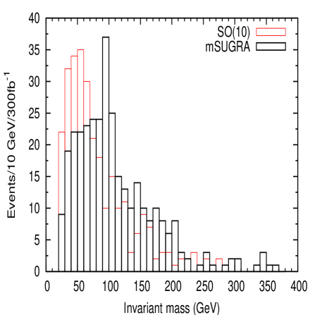
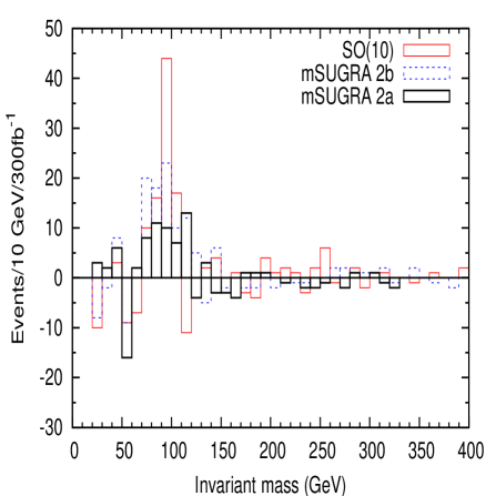
Figure 8: Left frame: The dilepton invariant mass distribution of opposite sign, same flavor dilepton events after cuts for point 1, corresponding to an integrated luminosity of 300 fb^-1; the black and red (grey) histograms are for the mSUGRA and $SO(10)$ versions of this point, respectively. Right Frame: The subtracted (OSSF$-$OSOF) dilepton invariant mass distribution after cuts for point 2; the solid black and dashed blue histograms are for the mSUGRA points 2a and 2b, while the solid red (grey) histogram is for the $SO(10)$ version.

The results of our simulations for point 1 are shown in the left frame of Figs. 8. We see that the di–lepton invariant mass distribution peaks near 50 GeV in the $SO(10)$ scenario, whereas it peaks at $M_{Z}$ in the mSUGRA scenario. mSUGRA also predicts a somewhat larger number of events at large di–lepton invariant mass; we saw above that only in this scenario we expect significant numbers of on–shell $W^{\pm}$ bosons from chargino and neutralino decay. The two distributions should be easily distinguishable, with high statistical significance, once several hundred fb^-1 of data will have been collected.

3.2.2 Point 2

We now turn to benchmark point 2. We saw in Table 1 that now $\tilde{\chi}_{2}^{0}\rightarrow\tilde{e}_{R}^{\pm}e^{\mp}$ are allowed in the mSUGRA scenarios, but not in $SO(10)$. Unfortunately, the branching ratios for these decays remain at the permille level even in the mSUGRA scenarios. This is partly due to the small phase space available for these decays, but mostly due to the fact that $\tilde{\chi}_{2}^{0}$ is dominantly a neutral wino in the co–annihilation region, and thus has only small couplings to $SU(2)$ singlet sleptons; recall that $\tilde{\tau}_{1}$ also has a significant $SU(2)$ doublet, $\tilde{\tau}_{L}$ component. As a result, we do not see any evidence for $\tilde{\chi}_{2}^{0}\rightarrow\tilde{\ell}_{R}^{\pm}\ell^{\mp}\rightarrow\tilde{\chi}_{1}^{0}\ell^{\pm}\ell^{\mp}\ (\ell=e,\ \mu)$ in the mSUGRA scenarios; in particular, no kinematic edge at $m_{\ell^{+}\ell^{-}}=189$ GeV, the nominal endpoint for this decay chain, is visible.

We instead first try to find the evidence for increased gaugino–higgsino mixing in the $SO(10)$ scenario, due to the lower value of $\mu$, by analyzing the decays of the heavier charginos and neutralinos. In the case at hand the dominant production channel is associate production of a first generation squark with a gluino. The decays of first and second generation squarks will predominantly produce $\tilde{\chi}_{1,2}^{0}$ and $\tilde{\chi}_{1}^{\pm}$ states. On the other hand, here in the co–annihilation region gluinos are heavier than all squarks, but – as usual in scenarios where squark masses unify at some high scale [35] – gluino decays into third generation quarks and squarks are preferred. We saw in the discussion of benchmark point 1 that third generation squarks in turn frequently decay into higgsino–like charginos and neutralinos. We look for these heavier states through their decays into real $Z^{0}$ bosons.

Modes	$SO(10)$ 2	mSUGRA 2a	mSUGRA 2b
$\tilde{g}\to\tilde{b}_{1}\bar{b}$	12.3 %	11.8 %	12.0 %
$\tilde{g}\to\tilde{b}_{2}\bar{b}$	7.0 %	6.2 %	6.2 %
$\tilde{g}\to\tilde{t}_{1}\bar{t}$	12.3 %	12.5 %	11.8 %
$\tilde{g}\to\tilde{t}_{2}\bar{t}$	2.9 %	-	-
$\tilde{t}_{1}\to\tilde{\chi}_{3}^{0}t$	18.1 %	5.2 %	13.6 %
$\tilde{t}_{1}\to\tilde{\chi}_{2}^{+}b$	21.9 %	21.3 %	22.5 %
$\tilde{t}_{2}\to\tilde{\chi}_{3}^{0}t$	10.4 %	8.0 %	8.9 %
$\tilde{t}_{2}\to\tilde{\chi}_{2}^{+}b$	24.8 %	20.4 %	22.6 %
$\tilde{t}_{2}\to Z^{0}\tilde{t}_{1}$	7.4 %	9.3 %	7.5 %
$\tilde{b}_{1}\to\tilde{\chi}_{3}^{0}b$	14.6 %	10.7 %	12.2 %
$\tilde{b}_{1}\to\tilde{\chi}_{2}^{-}t$	14.5 %	8.7 %	9.8 %
$\tilde{b}_{2}\to\tilde{\chi}_{3}^{0}b$	14.6 %	11.9 %	12.9 %
$\tilde{b}_{2}\to\tilde{\chi}_{2}^{-}t$	46.1 %	39.0 %	40.9 %
$\tilde{\chi}_{3}^{0}\to\tilde{\chi}_{1,2}^{0}Z^{0}$	29.3 %	28.0 %	28.0 %
$\tilde{\chi}_{2}^{+}\to\tilde{\chi}_{1}^{+}Z^{0}$	23.8 %	22.8 %	22.4 %
$\tilde{g}\to Z^{0}X$	7.6%	4.3%	5.0 %

Table 2: Branching ratios for important modes in benchmark point 2, as calculated with ISAJET 7.78 [36]; note that charge conjugate gluino decay modes have to be added. The last line denotes the sum of the branching ratios of all gluino decay chains which give us a $Z$ boson in the final state.

The relevant branching ratios are summarized in Table 2. We see that the slightly reduced third generation squark masses of the $SO(10)$ scenario increase the branching ratio for gluino decays into the third generation to 69% in the $SO(10)$ case, compared to 61% (60%) in mSUGRA point 2a (2b). Moreover, the decays of third generation squarks into $\tilde{\chi}_{3}^{0}$ and $\tilde{\chi}_{2}^{\pm}$ are enhanced in the $SO(10)$ case. This is also predominantly a phase space effect; the slightly reduced squark masses in the $SO(10)$ case are over–compensated by the reduced masses of the higgsino–like states. This effect is especially drastic for $\tilde{t}_{1}\rightarrow\tilde{\chi}_{3}^{0}t$, where the available phase space volume is very small in the mSUGRA scenarios. However, the strong phase space dependence of the relevant partial widths [6] leads to quite significant differences also in many other modes. Finally, the smaller value of $\mu$ in the $SO(10)$ scenario also leads to more higgsino–gaugino mixing, and hence to slightly larger branching ratios for decays of the heavier neutralinos and charginos into real $Z^{0}$ bosons. The combination of these three effects leads to a substantially larger $Z^{0}$ production rate in gluino cascade decays in the $SO(10)$ scenario than in mSUGRA.

In order to suppress backgrounds, we first make use of the fact that most signal events will have (at least) one very energetic jet from the decay of a first generation squark into a light gaugino–like state. Moreover, the above discussion shows that many events with real $Z^{0}$ bosons in the final state also will have a top quark in the final state, and/or a real $W^{\pm}$ boson from $\tilde{\chi}_{1}^{\pm}$ decay; the branching ratio for this latter decay amounts to 12.6% in the $SO(10)$ scenario. The decays of these particles can lead to additional, somewhat softer, jets and/or additional leptons. On the other hand, since the dominant production channel only contains a single gluino, we only expect two $b$ (anti–)quarks in the final state; $b-$tagging will therefore not be of much help to suppress the $t\bar{t}$ background, which we again expect to be the most dangerous one.

This leads us to use two complementary sets of cuts; at the end we simply add both event samples in order to increase the statistics:

1. Set 1

   • $E_{T}(j_{1})>600$ GeV, $E_{T}(j_{2})>200$ GeV, $E_{T}(j_{3})>100$ GeV.

   • $N_{\ell}=2$.

2. Set 2

   • $E_{T}(j_{1})>300$ GeV, $E_{T}(j_{2})>150$ GeV, $E_{T}(j_{3})>75$ GeV.

   • $N_{\ell}\geq 3$.

Note that we do not apply any cut on missing $E_{T}$, since this wasn’t necessary to suppress the backgrounds we studied. In Set 1, a modest missing $E_{T}$ cut will be needed to suppress the $Z^{0}+$jets background, but this can be done without any significant loss of signal.

For set 1, we require both charged leptons to be of opposite charge. In set 2, we chose the opposite–sign lepton pair whose invariant mass is closer to $M_{Z}$ as “$Z^{0}$ candidate”. We found that the background from $t\bar{t}$ is almost entirely removed by either set of cuts. Furthermore, in order to extract the lepton pairs from the decays of $Z^{0}$ bosons, we subtract the events with opposite sign opposite flavor (OSOF) lepton pairs. This removes SUSY backgrounds where the two leptons originate from independent (semi–)leptonic decays; in benchmark point 2, these come primarily from the decays of $W^{\pm}$ bosons.

The resulting di–lepton invariant mass spectrum is shown in the right frame of Fig. 8, for an integrated luminosity of 300 fb^-1. We see that the $Z^{0}$ peak is indeed much more pronounced in the $SO(10)$ scenario than in the two mSUGRA scenarios. This allows to distinguish between $SO(10)$ and mSUGRA at about $3\sigma$ statistical significance in this case.

As noted above, in the $SO(10)$ point 2, we find a branching ratio for $\tilde{\chi}_{1}^{\pm}\rightarrow W^{\pm}\tilde{\chi}_{1}^{0}$ of about 12.6%. In the mSUGRA points 2a and 2b, this branching ratio is only 6.1% and 6.6%, respectively. At an $e^{+}e^{-}$ linear collider with sufficient energy to produce $\tilde{\chi}_{1}^{+}\tilde{\chi}_{1}^{-}$ pairs this large difference in branching ratios should be straightforward to measure.

At the LHC we have to pursue a somewhat different strategy: leptonic decays of these $W^{\pm}$ can give rise to events with two leptons of the same charge (like–sign di–lepton events). These can originate from associate $\tilde{q}_{L}\tilde{g}$ production where $\tilde{g}$ decay also produces a lepton; the charge of this lepton from gluino decay is uncorrelated to that from squark decay, i.e. half the time the two leptons will have the same charge. The results of Table 2 indicate that the inclusive branching ratio for $\tilde{g}\rightarrow\ell^{\pm}$ is somewhat higher in the $SO(10)$ scenario than in both mSUGRA analogues. Other sources are $\tilde{u}_{L}\tilde{u}_{L}$ and $\tilde{d}_{L}\tilde{d}_{L}$ production, which give rise to $\ell^{+}\ell^{+}$ and $\ell^{-}\ell^{-}$ pairs, respectively, if both squarks decay into $\tilde{\chi}_{1}^{\pm}$. Of course, gluino pairs can also produce like–sign dileptons, but the gluino pair production cross section is relatively small at this benchmark point. Note also that the physics background for like–sign dileptons events is very small.

We applied the following cuts to isolate a clean sample of SUSY events:

• At least two jets, with $E_{T}(j_{1})>500$ GeV, $E_{T}(j_{2})>200$ GeV. These cuts are quite asymmetric, since we expect at least one very energetic jet from $\tilde{q}_{L}$ decay in the event.

• Exactly two equally charged isolated leptons, with $p_{T}(\ell)>10$ GeV as before.

With these cuts, we find 492 events in 300 fb^-1 for the $SO(10)$ scenario, as compared to 422 and 434 events in mSUGRA 2a and 2b, respectively. This difference of $\sim 3$ statistical standard deviations is much less than the above discussion would lead one to expect. The reason is that there is another large source of $\ell^{\pm}$ from $\tilde{q}_{L}$ decay: $\tilde{q}_{L}\rightarrow q\tilde{\chi}_{2}^{0}$ with $\tilde{\chi}_{2}^{0}\rightarrow\tau^{\pm}\tilde{\tau}_{1}^{\mp}$, and $\tau^{\pm}\rightarrow\ell^{\pm}\nu\bar{\nu}$. Unfortunately the branching ratios for these decays are somewhat larger in mSUGRA than in the $SO(10)$ scenario, because higgsino–gaugino mixing tends to suppress the corresponding partial widths. This significantly reduces the difference between the predictions for the total like–sign dilepton event rate.

One can imagine two strategies to enhance the difference between the predictions. One possibility is to veto leptons from $\tilde{\chi}_{2}^{0}\rightarrow\tau^{\pm}\tilde{\tau}_{1}^{\mp}$ decays by vetoing against the secondary $\tau^{\mp}$ from $\tilde{\tau}_{1}^{\mp}$ decay. However, this $\tau$ will be quite soft, so it is not clear how efficient such a $\tau$ veto would be. Another possibility is to subtract this source of hard leptons, by using events with an identified $\tau$ jet and the known $\tau$ decay branching ratios. Again, the feasibility of this method depends on $\tau$ tagging efficiencies and their uncertainties. We do therefore not pursue this strategy any further.

3.3 Measurements involving Higgs bosons at the LHC

Our benchmark points have quite large values of $\tan\beta$. This increases the cross sections for inclusive $gg\rightarrow A,\,H$ production, and for associate $gg\rightarrow b\bar{b}(A,\,H)$ production. The heavy Higgs bosons can be searched for using their decays into $\tau^{+}\tau^{-}$. According to simulations by the CMS collaboration [37], for $\tan\beta=40$ this would allow discovery of the heavy Higgs bosons out to $m_{A}\simeq 650$ GeV with 60 fb^-1 of data. In particular, we expect a robust signal for $H,\,A$ production in the mSUGRA version of benchmark point 1, but not in the $SO(10)$ version. In benchmark point 2, we expect signals of comparable size in all three cases. The $\tau^{+}\tau^{-}$ invariant mass resolution should suffice to distinguish between the $SO(10)$ and mSUGRA 2a scenarios, but distinguishing the $SO(10)$ scenario from mSUGRA 2b might be challenging.

In benchmark point 2, $\tilde{\chi}_{2}^{0}\to\tilde{\chi}_{1}^{0}+h$ decays might also allow to discriminate between $SO(10)$ and the two mSUGRA analogues. The branching ratio for this decay is 11.5% in the $SO(10)$ case, but only 5.3% (5.7%) for mSUGRA 2a (2b). About 90% of the light Higgs bosons will decay into $b\bar{b}$ pairs. Recall, however, that in this scenario gluino decays frequently lead to $b\bar{b}$ pairs in the final state, giving rise to a large SUSY background. We have therefore not pursued this avenue further.

4 Summary and Conclusions

We have investigated the detectability of neutralino Dark Matter and some LHC signatures for a SUSY$-SO(10)$ model with two intermediate scales, and compared results with the frequently analyzed mSUGRA model.

In Sec. 2 we have shown that in the cosmologically allowed region with large scalar mass parameter $m_{0}$, the direct detection of Dark Matter should be possible for the next generation of detectors, at least for gluino masses up to 2 TeV. In this region of parameter space, which corresponds to the “focus point” region of mSUGRA, IceCUBE will be able to detect the neutrino-induced muon flux from neutralino annihilation in the Sun. However, in this region of parameter space the Dark Matter detection rates predicted in the $SO(10)$ scenario are quite similar to those in mSUGRA, if one adjusts parameters such that the physical LSP mass and relic density is the same in both cases. On the other hand, in the co–annihilation region prospects for direct Dark Matter detection are much better in the $SO(10)$ case, although the cross section still remains somewhat below the projected sensitivity of next generation experiments. Unfortunately, in this case the neutrino signal from the Sun is several orders of magnitude below the IceCUBE sensitivity.

We also analyzed the flux of antiprotons from neutralino annihilation in the halo of our galaxy. Even in the most optimistic case – with a large annihilation cross section, and a halo profile strongly peaked at the galactic center – the predicted flux falls well below the flux extracted from the PAMELA $\bar{p}/p$ flux ratio and the known proton flux. Given the large uncertainties in both signal and background, searches for antimatter do not appear to be very promising Dark Matter search channels in this scenario.

In Sec. 3 we compared some collider signals from the model with those of mSUGRA. We chose two benchmark points, one of which resembles a “focus point” scenario, while the other lies in the co–annihilation region. We compared those with mSUGRA points with identical gluino and first generation squark masses, and (almost) identical neutralino relic density. We showed that events containing hard jets and two (or more) charged leptons (electrons and muons) can be used to discriminate between mSUGRA and our $SO(10)$ benchmark points. The existence and size of a $Z^{0}$ peak in the di–lepton invariant mass distribution proved particularly useful. Moreover, in the first benchmark point the search for heavy neutral MSSM Higgs bosons can help to discriminate between the $SO(10)$ and mSUGRA models, whereas in the second point the number of like–sign dilepton events can be used.

It may be interesting to note that searching for events containing leptonically decaying $Z^{0}$ bosons [38] or like–sign dileptons [39] were the first strategies suggested to look for cascade decays of heavy squarks and gluinos. It was realized later that other channels with fewer leptons offer better SUSY discovery reach [40, 24]. Here we find that $Z^{0}$ bosons and like–sign lepton pairs can be very useful for discriminating between different SUSY models.

In the co–annihilation region, the physical spectra predicted by $SO(10)$ and mSUGRA are quite similar. The models differ mostly in the values of $\mu$ derived via electroweak symmetry breaking; the $SO(10)$ scenario also predicts somewhat reduced masses for third generation squarks. The fact that our analyses nevertheless led to significant differences in several signals bodes well for the power of LHC experiments to distinguish between competing SUSY models. However, we have not attempted to distinguish the $SO(10)$ model from other modifications of mSUGRA, e.g. scenarios with non–universal soft masses for Higgs bosons [41], which also lead to variations in $\mu$ as well as the masses of third generation sfermions and Higgs bosons.

Indeed, it is clearly impossible to distinguish our model from sufficiently complicated SUGRA scenarios with non–universal scalar soft breaking masses using superparticle and Higgs boson properties only, simply because the two models can have identical weak–scale spectra. Recall, however, that our model also makes other predictions. For the chosen (extreme) value of the scale of Grand Unification, proton decay should be within reach of next generation experiments [42]. This low unification scale also implies a rather large mass for at least one neutrino; this can be probed using cosmological data [43], and perhaps even through laboratory experiments [44]. By combining all the information, we will hopefully be able to pin down the physics at the Grand Unified scale.

Acknowledgments

We thank Siba P. Das for helpful discussions on the use of PYTHIA, and Stefano Profumo for discussions on the detectability of neutralino Dark Matter by antimatter search experiments. MD and JMK are partially supported by the Marie Curie Training Research Networks “UniverseNet” under contract no. MRTN-CT-2006-035863, and “UniLHC” under contract no. PITN-GA-2009-237920. EKP acknowledges the hospitality of LAPTH and LPSC while part of this work was done.

References

- [1] H. Fritzsch and P. Minkowski, Ann. Phys. 93 (1975) 193; M.S. Chanowitz, J. Ellis and M.K. Gaillard, Nucl. Phys. B128 (1977) 506.
- [2] P. Minkowski, Phys. Lett. B 67 (1977) 421
- [3] M. Drees and J.M. Kim, JHEP 0812 (2008) 095, arXiv:0810.1875 [hep-ph].
- [4] C.S. Aulakh, B. Bajc, A. Melfo, A. Rasin and G. Senjanovic, Nucl. Phys. B597 (2001) 89, hep–ph/0004031.
- [5] Particle Data Group, C. Amsler et al., Phys. Lett. B667 (2008) 1.
- [6] For introductions to supersymmetry in general, and to mSUGRA in particular, see e.g. M. Drees, R.M. Godbole and P. Roy, Theory and Phenomenology of Sparticles, World Scientific (2004); H. Baer and X. Tata, Weak scale supersymmetry: From superfields to scattering events, Cambridge, UK University Press (2006).
- [7] B.C. Allanach, Comput. Phys. Commun. 143 (2002) 305, hep–ph/0104145.
- [8] G. Bélanger, F. Boudjema, A. Pukhov and A. Semenov, Comput. Phys. Commun. 176 (2007) 367, hep–ph/0607059.
- [9] P. Gondolo, J. Edsjo, P. Ullio, L. Bergström, M. Schelke and E.A. Baltz, JCAP 0407 (2004) 008, arXiv:astro-ph/0406204; P. Gondolo, J. Edsjö, P. Ullio, L. Bergström, M. Schelke, E.A. Baltz, T. Bringmann and G. Duda, http://www.physto.se/ edsjo/darksusy
- [10] For a review of neutralino Dark Matter detection, see G. Jungman, M. Kamionkowski and K. Griest, Phys. Rep. 267 (1996) 195, hep–ph/9506380.
- [11] WMAP Collab., E. Komatsu et al., Astrophys. J. Suppl. 180 (2009) 330, arXiv:0803.0547 [astro–ph].
- [12] R. Gaitskell and J. Filippini, http://dmtools.berkeley.edu/limitplots/
- [13] CDMS–II Collab., Z. Ahmed et al., arXiv:0912.3592 [astro–ph.CO].
- [14] J.L. Feng, K.T. Matchev and T. Moroi, Phys. Rev. D61 (2000) 075005, hep–ph/9909334; J.L. Feng, K.T. Matchev and F. Wilczek, Phys. Lett. B482 (2000) 388, hep–ph/0004043.
- [15] J.R. Ellis, T. Falk, and K.A. Olive, Phys. Lett. B444 (1998) 367, hep–ph/9810360; J.R. Ellis, T. Falk, K.A. Olive and M. Srednicki, Astropart. Phys. 13 (2000) 181, Erratum-ibid. 15 (2001) 413, hep–ph/9905481; M.E. Gomez, G. Lazarides and C. Pallis, Phys. Rev. D61 (2000) 123512, hep–ph/9907261.
- [16] IceCUBE Collab., arXiv:0711.0353 [astro–ph].
- [17] J. Edsjo, M. Schelke and P. Ullio, JCAP 0409 (2004) 004, astro–ph/0405414.
- [18] J.F. Navarro et al., Mon. Not. Roy. Astron. Soc. 349 (2004) 1039, astro–ph/0311231.
- [19] A. Burkert, Astrophys. J. 447 (1995) L25.
- [20] J.F. Navarro, C.S. Frenk and S.D.M. White, Astrophys. J. 462 (1996) 563, and Astrophys. J. 490 (1997) 493.
- [21] S. Profumo and P. Ullio, JCAP 0407 (2004) 006, hep–ph/0406018.
- [22] PAMELA Collab., O. Adriani et al., Phys. Rev. Lett. 102 (2009) 051101, arXiv:0810.4994 [astro–ph].
- [23] H. Baer, A. Belyaev, T. Krupovnickas and J. O’Farrill, JCAP 0408 (2004) 005, hep–ph/0405210.
- [24] For a recent detailed assessment of the mSUGRA discovery potential of LHC experiments, see H. Baer, V. Barger, A. Lessa and X. Tata, JHEP 0909 (2009) 063, arXiv:0907.1922 [hep–ph].
- [25] See e.g. M. Davier, arXiv:1001.2243 [hep–ph]; T. Teubner, K. Hagiwara, R. Liao, A.D. Martin and D. Nomura, arXiv:1001.5401 [hep–ph]; and references therein.
- [26] M. Drees and M.M. Nojiri, Phys. Rev. D47 (1993) 376, hep–ph/9207234.
- [27] M.M. Nojiri, Phys. Rev. D 51 (1995) 6281, hep–ph/9412374.
- [28] B.K. Bullock, K. Hagiwara and A.D. Martin, Nucl. Phys. B395 (1993) 499.
- [29] R.M. Godbole, M. Guchait and D.P. Roy, Phys. Lett. B618 (2005) 193, hep–ph/0411306.
- [30] M. Guchait and D.P. Roy, Phys. Lett. B541 (2002) 356, hep–ph/0205015.
- [31] F. del Aguila and L. Ametller, Phys. Lett. B261 (1991) 326; H. Baer, C.-h. Chen, F. Paige and X. Tata, Phys. Rev. D49 (1994) 3283, hep–ph/9311248.
- [32] H. Baer, C.-h. Chen, F. Paige and X. Tata, Phys. Rev. D50 (1994) 4508, hep–ph/9404212.
- [33] T. Sjöstrand, S. Mrenna and P. Skands, JHEP 0605 (2006) 026, hep–ph/0603175.
- [34] ATLAS Collab., G. Aad et al., arXiv:0901.0512 [hep-ex].
- [35] M. Drees and M.M. Nojiri, Nucl. Phys. B369 (1992) 54.
- [36] F.E. Paige, S.D. Protopopescu, H. Baer and X. Tata, hep–ph/0312045.
- [37] CMS Collab., A. De Roeck et al., CMS Physics Technical Design Report, Vol. II, Sec. 11.3; see http://cdsweb.cern.ch/record/942733/files/lhcc-2006-021.pdf
- [38] H. Baer, V.D. Barger, D. Karatas and X. Tata, Phys. Rev. D36 (1987) 96.
- [39] R.M. Barnett, J.F. Gunion and H.E. Haber, Phys. Lett. B315 (1993) 349, hep–ph/9306204.
- [40] H. Baer, C.-h. Chen, F. Paige and X. Tata, Phys. Rev. D52 (1995) 2746, hep–ph/9503271, and Phys. Rev. D53 (1996) 6241, hep–ph/9512383.
- [41] M. Drees, Y.G. Kim, M.M. Nojiri, D. Toya, K. Hasuko and T. Kobayashi, Phys. Rev. D63 (2001) 035008, hep–ph/0007202; J.R. Ellis, T. Falk, K.A. Olive and Y. Santoso, Nucl. Phys. B652 (2003) 259, hep–ph/0210205; H. Baer, A. Mustafayev, S. Profumo, A. Belyaev and X. Tata, JHEP 0507 (2005) 065, hep–ph/0504001.
- [42] See e.g. K. Nakamura, Front. Phys. 35 (2000) 359; A. Bueno et al., JHEP 0704 (2007) 041, hep–ph/0701101.
- [43] See e.g. S. Hannestad and Y.Y.Y. Wong, JCAP 0707 (2007) 004, astro–ph/0703031.
- [44] G. Drexlin for the KATRIN Collab., Nucl. Phys. Proc. Suppl. 145 (2005) 263.