Incoherent MAR in an array of SNS junctions. N. M. Chtchelkatchev N. M. Chtchelkatchev *

Incoherent multiple Andreev reflection in an array of SNS junctions.

Abstract

Last years many interesting effects related to incoherent MAR have been experimentally found, but only few of them were theoretically explained. It was shown, for example, that if the voltage at the edges of a linear array is $V$ then subgarmonic structures in the current -voltage characteristics appear not only at usual for nonstationary Josephson effect positions, $V_{n}=2\Delta/n$, where $n$ is integer, but also at voltages other than $V_{n}$. A step towards description of electron transport in a dirty array of SNS junctions is done in this letter. It is shown that subgarmonic structures may indeed appear at “unusual” voltages.

73.23.-b, 74.45.+c, 74.81.Fa

Important role plays Andreev reflection mechanism in the subgap charge transfer through a normal metal (N) – superconductor (S) junction [1]. When an electron quasiparticle in a normal metal with the energy below the superconduting gap reflects from the interface of the superconductor into a hole, Cooper pair transfers into the superconductor. If the normal metal is surrounded by superconductors, so we have a SNS junction, a number of Andreev reflections appear at the NS interfaces. In equilibrium this leads to Andreev quasiparticle levels in the normal metal that carry considerable part of the Josephson current; out of the equilibrium, when superconductors are voltage biased, quasiparticles Andreev reflect about $2\Delta/eV$ times transferring large quanta of charge ($\sim 2e\cdot[2\Delta/eV]$) from one superconductor to the other. This effect is called Multiple Andreev Reflection (MAR). If the voltage is near $V_{n}=2\Delta/n$, where $n=1,2,\ldots$, so-called subgap features in current voltage characteristics appear. Then large contribution to the current give quasiparticles that go from the gap edge of one superconductor to the gap edge of the other superconductor (after MAR in the normal region); bulk superconductor DoS is large at the gap and this is the reason of subgap features.

This letter is devoted to investigation of electron transport in arrays of dirty superconductiong mesoscopic SNS (SFS) junctions. I assume that normal parts of the junctions are “long”. It implies that minimum distance $d_{0}$ between adjacent superconductors is much larger than the characteristic scale of anomalous green function (Cooper pair wave function) decay $\xi_{N}$ from a superconductor in the normal metal. If the diffusion coefficient of the normal metal is $D_{N}$ than $\xi_{N}\sim\sqrt{D_{N}/T}\ll d_{0}$, where $T$ is the temperature. Energy relaxation is not included in the calculations. So it is also assumed that the array is not large, its characteristic length does not exceed the characteristic length scale of quasiparticle energy relaxation in the normal metal and in superconductors. [Quasiparticle energy relaxation was “taken into account” in Ref.[4], where incoherent MAR in long SNS junction was discussed, by small imaginary part supplied to the energy in retarded and advanced greens functions; but collisional integrals were not taken into account in kinetic equations. It is not clear why this procedure is correct. I do not follow this way here.] Conditions listed above also mean that in equillibrium the proximity (Josephson) effect between the superconducors is suppressed. Josephson current, for example, is exponentially small with $d_{0}/\xi_{N}$. It is known that out of the equilibrium when there is a finite bias between the superconducors the proximity effect restores in some sense: subgap features appear due to MAR in current-voltage characteristics. MAR in long Josephson junctions usually is referred to as ‘incoherent” since there is no contribution to electron transport from effects related to interference of quasiparticle wave functions in normal metals (contrary to Josephson effect in “short” superconducting junctions). Last years many interesting effects related to incoherent MAR have been experimentally found, but only few of them were theoretically explained. It was shown, for example, that if the voltage at the edges of a linear array is $V$ then subgarmonic structures in the current -voltage characteristics appear not only at usual for nonstationary Josephson effect positions, $V_{n}=2\Delta/n$, where $n$ is integer, but also at voltages other than $V_{n}$, see Ref.[2] and refs. therein. A step towards description of electron transport in a dirty array of SNS junctions is done in this letter. It is shown that subgarmonic structures may indeed appear at “unusual” voltages.

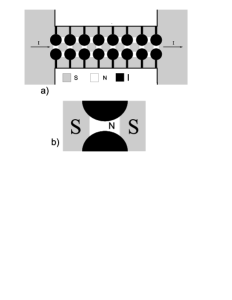
Figure 1: Fig.1. a) An array of SNS junctions, like in experiments [2]. b) A sketch of the normal layer connection to the superconductors in experimental SNS arrays. Black area is insulating.

Investigation of electron transport is based on Usadel equations:

$$[\check{H},\check{G}]=iD\nabla\cdot\mathbf{\check{J}},\qquad\mathbf{\check{J}}=\check{G}\nabla\check{G},\qquad\check{G}^{2}=\check{1},$$ (1)

$$\check{H}=\check{1}(i\hat{\sigma}_{z}\partial_{t}-e\phi+\hat{\Delta}),$$ (2)

$$\hat{\Delta}=\begin{pmatrix}0&\Delta\\ -\Delta^{*}&0\\ \end{pmatrix},$$ (3)

$$I(t,x)=\frac{\pi\hbar\sigma_{{}_{N}}}{4e}\operatorname{Tr}\hat{\sigma}_{z}\hat{J}^{K}(t,t;x),$$ (4)

where

$$\check{G}=\begin{pmatrix}\hat{R}&\hat{K}\\ 0&\hat{A}\\ \end{pmatrix}.$$ (5)

Here $\hat{R}$, $\hat{K}$ and $\hat{A}$ denote retarded, Keldysh and advanced quasiclassical green functions. The hat reminds that greens function are in turn matrices in Nambu space. $\hat{\sigma}$ are Pauli matrices that act in Nambu space; $D$ is a diffusion coefficient that equals $D_{N}$ in a normal metal and $D_{S}$ in a superconductor; $\Delta$ is the superconducting gap; $\phi$ is electrical potential; $\sigma_{N}$ is the conductivity of a normal metal. The boundary conditions for the Usadel equations at NS interfaces are:

$$\sigma_{{}_{N_{2}}}\check{\mathbf{J}}_{2}\cdot\mathbf{n}_{2}=\frac{G_{12}}{2}[\check{G}_{2},\check{G}_{1}]_{-},$$ (6)

where $1,2$ label interface sides, $G_{12}$ is the surface conductance and $\mathbf{n}_{2}$ is the unit normal to the interface pointing to the second half-space.

The problem is to calculate the current in a long SNS array using Eqs.(1)-(6). Solving these equations directly is a hard task because they are nonlinear, nonuniform and essentially time dependent (relative phases of superconductors rotate with biases). So the main task is developing an approach for the problem in hand that allows to perform significant part of transport calculations analytically and that is applicable in rather wide range of system parameters. There is no universal approach that helps to solve Usadel equations analytically, so any analytical method of Usadel equations solution is usually specific to the given class of the physical systems.

Normal layers in experimental SNS arrays [2] connect with superconductors like it is shown in Fig.1. SNS junctions of this type are usually referred to as “weak-links” [3]. Boundary conditions, Eq.(6), can be simplified in this case: retarded and advanced Greens functions at superconducting sides of NS boundaries can be substituted by Greens function from the bulk of the superconductors. These “rigid” boundary conditions approximation are reasonable because a) the magnitude of the current is much smaller than the critical current of the superconductor (this is assumed), b) the current entering the superconductor from narrow normal metal wire [the width $\lesssim\xi=\sqrt{D_{S}/T_{c}}$, where $T_{c}$ is the critical temperature of the superconductor] spreads nearly at the NS interface over the whole superconductor. There are also other cases when rigid boundary conditions are correct, for example, if the NS boundary has small transparency due to an insulator layer or other reasons.

The Keldysh greens function has the following general parametrization: $\hat{K}=\hat{R}\circ\hat{f}-\hat{f}\circ\hat{A}$, where $\hat{f}$ is the distribution function. It was shown in Ref.[4] that the current in a long SNS junction can be found from investigation of the current distribution in an effective network where the role of voltages play distribution functions made from components of $\hat{f}$, the role of resistances play NS resistances renormalized by proximity effect and normal layer resistances. This idea can be applied to an SNS array.

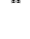
Figure 2: Fig.2. The simplest array of SNS junctions: SNSNS.

It is convenient to write $\hat{f}=\hat{1}f_{+}+\hat{\sigma}_{z}f_{-}$. Phases of the superconducting order parameters rotate with the biases so one could write in general $\hat{f}(\epsilon,\epsilon^{\prime})=\sum_{n=\{n_{i};i=1,2\ldots\}}\hat{f}_{n}(\epsilon-\epsilon^{\prime})\delta(\epsilon-\epsilon^{\prime}+n_{i}V_{i})$, where $n_{i}$ is integer, $V_{i}$ is the bias at the $i$’s superconductor. (Similar consideration apply for retarded and advanced greens functions.) However due to the absence of Josephson-type interference effects nonzero are only that $\hat{f}_{n}$ which provide time independent (dissipative) component of the current as it is well explained in Ref.[4]… One can write boundary conditions Eq.(6) at an NS interface for $\hat{f}_{n}$ as

$$\sigma_{N}D_{+}\nabla f_{+}^{(2)}=-G_{+}(f_{+}^{(2)}-f_{+}^{(1)}),$$ (7)

$$\sigma_{N}D_{-}\nabla f_{-}^{(2)}=-G_{-}(f_{-}^{(2)}-f_{-}^{(1)}).$$ (8)

Here the label 2 corresponds to the normal metal. For example,

$$D_{+}=\frac{1}{4}\operatorname{Tr}\left(\hat{1}-\hat{R}\hat{A}\right),$$ (9)

$$D_{-}=\frac{1}{4}\operatorname{Tr}\left(\hat{1}-\hat{R}\hat{\sigma}_{z}\hat{A}\hat{\sigma}_{z}\right).$$ (10)

Definitions of $G_{\pm}$ are similar and can be found, e.g., in Ref.[4].

It is useful to go from $f_{\pm}$ to $n_{e(h)}$ [4] that are related as follows: $f_{+}=1-(n_{e}+n_{h})$, $f_{-}=(n_{h}-n_{e})$. Then the boundary conditions, Eqs.(7), can be written as

$$\begin{split}I_{e}=G_{T}(n_{e}^{(1)}-&n_{e}^{(2)})-\\ -G_{A}(&(n_{e}^{(2)}-n_{h}^{(2)})-(n_{e}^{(1)}-n_{h}^{(1)})),\end{split}$$ (11)

$$\begin{split}I_{h}=G_{T}(n_{h}^{(1)}-&n_{h}^{(2)})+\\ +G_{A}(&(n_{e}^{(2)}-n_{h}^{(2)})-(n_{e}^{(1)}-n_{h}^{(1)})).\end{split}$$ (12)

Here $G_{T}=G_{+}$, $G_{A}=(G_{-}-G_{+})/2$ and $I_{e(h)}=-\sigma_{N}\frac{1}{2}(D_{+}\partial(n_{e}+n_{h})\pm D_{-}\partial(n_{e}-n_{h}))$. If the superconducting bank labelled by index “1” is in equilibrium, so $n_{e}^{(1)}=n_{h}^{(1)}=n_{F}$, then we arrive at boundary conditions written in Eq.(21) of Ref.[4]. If one writes Eqs.(11)-(12) for NS and SN interfaces of a superconducting island and uses conditions of electron and heat currents conservation in the island then quasiparticle distribution functions corresponding to superconducting islands can be excluded from boundary conditions:

$$I_{e}=A_{+}(n_{e}^{(2)}-n_{e}^{(1)})+A_{-}(n_{h}^{(2)}-n_{h}^{(1)}),$$ (13)

$$I_{h}=A_{+}(n_{h}^{(2)}-n_{h}^{(1)})+A_{-}(n_{e}^{(2)}-n_{e}^{(1)}).$$ (14)

It is worth noting that Eqs.(13)-(14) are derived for a linear array of SNS junctions; generalization of these equations is straightforward for more complicated arrays.

Figure 3: Fig.3. a) An illustration of the boundary conditions Eqs.(13)-(12) in terms of a circuit is given in Fig.3. Electron and hole currents entering the left side of the pyramid flow in one normal layer, the right currents flow in the other normal layer. $-A_{-}$ resistance describes Andreev reflection, $A_{+}$ — quasiparticle normal transmission through the superconductor and $A_{-}$ is Andreev transmission characteristics. b) An illustration of the boundary conditions Eqs.(13)-(12) (developed in Ref.[4]) at the surface of the superconductor connected to an electron reservoir , i.e., when $n_{e}^{(1)}=n_{h}^{(1)}=n_{F}$ in the superconductor. Here $R_{A}=1/G_{A}$, $R_{T}=1/G_{T}$.

In the last pair of equations labels 1 and 2 correspond to normal layers surrounding the superconducting island. Information that the island is superconducting is included in $A_{\pm}$ definition through $G_{\pm}$:

$$A_{\pm}=\frac{1}{2}(\mu_{+}\pm\mu_{-}),$$ (15)

$$\mu_{\pm}=\frac{G_{\pm}^{(1)}G_{\pm}^{(2)}}{G_{\pm}^{(1)}+G_{\pm}^{(2)}}.$$ (16)

A circuit illustration of this boundary condition is given in Fig.3a. Electron and hole currents entering the left side of the pyramid flow in one normal layer, the right currents flow in the other normal layer. $-A_{-}$ resistance describes Andreev reflection, $A_{+}$ — quasiparticle normal transmission through the superconductor and $A_{-}$ is Andreev transmission characteristics. It was assumed deriving Eqs.(13)-(12) that electrochemical potential within the superconductor is constant. This is correct if the characteristic distance between NS interfaces of the superconducting island is smaller than the electron disbalance characteristic length $\lambda_{Q}$[5]. It is implied that nonequillibrium quasiparticles above the gap do not have enough time for energy relaxation at their fly through the superconductor, so electrochemical potential within the superconductor is constant. Or if characteristic bias value $\delta V$ between adjacent superconducting islands is much smaller than the gap and the temperature is much below $T_{c}$ then most part of the current carry Cooper pairs through superconductors rather than quasiparticles above the gap. Then correction to the total current in the array from quasiparticle energy relaxation in superconductors is expected to be small as $\delta V/\Delta\ll 1$ and discussion related to $\lambda_{Q}$ is not relevant.

Next important step is expressing all boundary conditions in terms of the distribution functions $\bar{n}_{e(h)}$ [4], where

$$\overline{n}_{\pm}=n_{\pm}-\frac{I_{\pm}}{\sigma_{N}}\int_{0}^{\infty}dx^{\prime}\left(\frac{1}{D_{\pm}(x^{\prime})}-1\right)\equiv n_{\pm}-m_{\pm}I_{\pm}.$$

Here $n_{\pm}=n_{e}\pm n_{h}$ and $\bar{n}_{\pm}=\bar{n}_{e}\pm\bar{n}_{h}$, $D_{\pm}\partial f_{\pm}\equiv I_{\pm}/\sigma_{N}$. The integral here goes from the NS boundary ($x=0$) into the depth of the normal metal. Boundary conditions Eqs.(13)-(12) written in terms of $\bar{n}_{e(h)}$ will have the same form if one replaces $G_{\pm}$ by $\bar{G}_{\pm}={G_{\pm}}/({1+G_{\pm}m_{\pm}})$. Then

$$\bar{\mu}_{\pm}=\frac{\mu_{\pm}}{1+(m_{\pm}^{(2)}-m_{\pm}^{(1)})\mu_{\pm}},$$ (17)

where indices 1,2 correspond to two normal layers contacting with the superconducting island. It is useful to work with $\bar{n}_{e(h)}$ because then the proximity effect renormalization of the boundary resistances, $m_{\pm}$, is automatically taken into account.

The next step toward current calculation is to draw an effective network that describes MAR in the array of the junctions using Eqs.(13)-(12) and evaluate partial currents in this network using to Kirchhoff’s laws. Important task is to find voltages at the superconducting islands. But this can be found easily in several cases. For example, when the array consists of equal SNS junctions, or if most of the voltage drops at normal layers. Below these situations will be discussed. More complicated cases I leave for extended paper. If currents in the MAR network are found then electric current can be evaluated, e.g., as follows:

$$I=\frac{1}{2e}\int dE\left(I_{e}(E)-I_{h}(E)\right),$$ (18)

where $I_{e(h)}$ correspond to the normal layer at the edge of the array contacting with the superconducting reservoir with zero voltage.

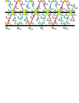
Figure 4: Fig.4. MAR in a SNSNS array with equal SNS junctions. The graph shows the effective circuit for quasiparticle currents in energy space. The role of voltages here play quasiparticle distribution functions. For example $n_{n}^{4}$ is the quasiparticle distribution function depending from $E+nV/2$; $U_{n}=n_{F}(E+nV/2)$. Boxes, triangles and ovals play the role of effective resistances that come from Usadel equations and their boundary conditions, Eqs.(1)-(6). The oval is the resistance of the normal layer. The box and the triangle correspond to the pyramidal bridge in Fig.3a and the three-terminal device in Fig.3b. The upper raw of $U$’s correspond to the first superconductor of the array, the lower raw – to the last superconductor. The thick line in the center of the graph represents the superconducting island.

The format of the letter does not allow to describe complicated arrays here, so one of the simplest SNS arrays, the SNSNS junction (Fig.2), will be considered below as an example. It will be shown how to construct an effective network that helps to describe its transport properties. Transport in more complicated arrays, like in Fig.1 can be described in a similar manner as for SNSNS; it will be demonstrated in an extended version of this paper.

Effective MAR network for a SNSNS junction like in Fig.2 is shown in Fig.4. The bias between the supercondcutors at the edges of the array is $V$. Then the bias of the central superconductor is $V/2$; it follows from symmetry reasons. Currents $I_{n}$ and $J_{n}$ correspond $I_{e}$ for lines beginning from $U_{n_{1}}$ and ending at $U_{n_{2}}$ with $n_{2}>n_{1}$ and $-I_{h}$ vice-versa. The role of voltages play quasiparticle distribution functions. For example $n_{n}^{4}$ is the quasiparticle distribution function depending from $E+nV/2$; $U_{n}=n_{F}(E+nV/2)$. Bars above the distribution functions are supposed but not shown explicitly in the figure. Boxes, triangles and ovals play the role of effective resistances (also with bars) that come from Usadel equations and their boundary conditions, Eqs.(1)-(6). The oval is the resistance of the normal layer. The box and the triangle correspond to the pyramidal bridge in Fig.3a and the three-terminal device in Fig.3b. The upper raw of $U$’s correspond to the first superconductor of the array, the lower raw – to the last superconductor. The thick line in the center of the graph represents the superconducting island.

Lets find recurrence relations for the currents $I_{n}$ and $J_{n}$. It follows from Fig.4 that

$$\begin{array}[]{rcl}I_{n}&=&\bar{G}_{T}^{n-2}(n_{n-2}^{4}-U_{n-2})+\bar{G}_{A}^{n-2}(n_{n-2}^{4}-n_{n-2}^{3}),\\ I_{n}&=&G_{N}(n_{n-1}^{3}-n_{n-2}^{4}),\\ I_{n}&=&A_{+}^{n-1}(n_{n-1}^{2}-n_{n-1}^{3})+A_{-}^{n-1}(n^{1}_{n-1}-n^{4}_{n-1}),\\ I_{n}&=&G_{N}(n_{n}^{1}-n_{n-1}^{2}),\\ I_{n}&=&\bar{G}_{T}^{n}(U_{n}-n_{n}^{1})+\bar{G}_{A}^{n}(n_{n}^{2}-n_{n}^{1}),\\ J_{n-2}&=&\bar{G}_{A}^{n-2}(n^{4}_{n-2}-n^{3}_{n-2})+\bar{G}_{T}^{n-2}(U_{n-2}-n^{3}_{n-2}),\\ J_{n+2}&=&\bar{G}_{A}^{n}(n^{2}_{n}-n^{1}_{n})+\bar{G}_{T}^{n}(n_{n}^{2}-U_{n});\end{array}$$ (26)

$$\begin{array}[]{rcl}J_{n}&=&\bar{G}_{T}^{n-2}(n_{n-2}^{2}-U_{n-2})+\bar{G}_{A}^{n-2}(n_{n-2}^{2}-n_{n-2}^{1}),\\ J_{n}&=&G_{N}(n_{n-1}^{1}-n_{n-2}^{2}),\\ J_{n}&=&A_{+}^{n-1}(n_{n-1}^{4}-n_{n-1}^{1})+A_{-}^{n-1}(n^{3}_{n-1}-n^{2}_{n-1}),\\ J_{n}&=&G_{N}(n_{n}^{3}-n_{n-1}^{4}),\\ J_{n}&=&\bar{G}_{T}^{n}(U_{n}-n_{n}^{3})+\bar{G}_{A}^{n}(n_{n}^{4}-n_{n}^{3}),\\ I_{n-2}&=&\bar{G}_{A}^{n-2}(n^{2}_{n-2}-n^{1}_{n-2})+\bar{G}_{T}^{n-2}(U_{n-2}-n^{1}_{n-2}),\\ I_{n+2}&=&\bar{G}_{A}^{n}(n^{4}_{n}-n^{3}_{n})+\bar{G}_{T}^{n}(n_{n}^{4}-U_{n}).\end{array}$$ (34)

Getting rid of the distribution functions in these set of equations one can get:

$$I_{n}\left(\frac{1}{A^{+}_{n-1}-A_{n-1}^{-}}+(a_{n}+a_{n-2})\right)-\\ -I_{n-2}b_{n-2}-I_{n+2}b_{n}=(U_{n}-U_{n-2}).$$ (35)

Same equation satisfies $J_{n}$. Here

$$a_{n}=\frac{1}{G_{N}}+\frac{1}{\bar{G}_{T}^{n}}-\frac{1}{2\bar{G}_{A}^{n}+\bar{G}_{T}^{n}}\frac{\bar{G}_{A}^{n}}{\bar{G}_{T}^{n}},$$ (36)

$$b_{n}=\frac{1}{2\bar{G}_{A}^{n}+\bar{G}_{T}^{n}}\frac{\bar{G}_{A}^{n}}{\bar{G}_{T}^{n}}.$$ (37)

Eq.(35) coincides with recurrence relation Eq.(52) from Ref.[4] derived for a single SNS junction if I replace in Eq.(52) $G_{N}$ by

$$\widetilde{G_{N}}=\frac{G_{N}}{2}\frac{{\bar{G}_{-}}}{G_{N}+{\bar{G}_{-}}}.$$ (38)

It means that SNSNS array behaves similarly as a single SNS junction but with energy dependent resistance of the normal layer. $\bar{G}_{-}$ has singularities at energy corresponding to the gap edges of the superconducting island in the center of the SNSNS array. This is the reason of subharmonic singularities in current voltage characteristics if $2\Delta/V=n/2$, $n=1,2,\ldots$ instead of “usual” positions,$2\Delta/V=n$; Fig.5 illustrates it. From Eq.(38) follows that unusual position of subharmonic singularities disappear if $\tilde{G}_{N}\to G_{N}$ if the resistance of the normal layer exceeds the resistance of SN interfaces. Then the central superconducting island of the SNSNS array effectively “disappear”. It was checked if the exchange field in SFSFS junction splits subharmonic structure; there was found no exchange field splitting effects because configurations of the ferromagnet and the superconductor like in Fig.1 does not lead to enough exchange field deformation of superconductor DoS near SF boundary that is necessary for the splitting effect observation. This paragraph is conclusion of the paper.

Figure 5: Fig.5. Subharmonic structure in differential conductivity of SNSNS junction with the ratio $r$ of SN boundary resistance to normal layer resistance $R_{N}$, $r=0.2$. Peaks at half-integer $2\Delta/V$ do not appear in $dI/dV$ of SNS junctions.

I’m grateful to T.Baturina and I.S. Burmistrov for stimulating discussions. I especially thank I. Drebushchak for helpful discussions and the idea to draw Fig.3. I also thank RFBR 03-02-16677, the Russian Ministry of Science, the Netherlands Organization for Scientific Research (NWO), CRDF and Russian Science Support foundation.

References

- [1] A.F.Andreev, Zh. Éksp. Teor. Fiz. 46, 1823 (1964) [Sov. Phys. JETP 19, 1228 (1964)].
- [2] T.I. Baturina, Yu. A. Tsaplin, A.E. Plotnikov et al, JETP Lett. 81, 10 (2005); T.I. Baturina, D.R. Islamov, Z.D. Kvon, JETP Lett. 75, 326 (2002). T.I. Baturina, Z.D. Kvon, A.E. Plotnikov, Phys. Rev. B 63, 180503 (2001).
- [3] K.K. Likharev, Rev. Mod. Phys. 51, 101 (1979).
- [4] E.V. Bezuglyi, E.N. Bratus , V.S. Shumeiko et al, Phys.Rev. B 62, 14439 (2002).
- [5] M.Tinkham, Introduction to superconductivity, Mc.Graw-Hill Inc., 1996.