Collision of Polymers in a Vacuum

Abstract

In a number of experimental situations, single polymer molecules can be suspended in a vacuum. Here collisions between such molecules are considered. The limit of high collision velocity is investigated numerically for a variety of conditions. The distribution of contact times, scattering angles, and final velocities are analyzed. In this limit, self avoiding chains are found to become highly stretched as they collide with each other, and have a distribution of scattering times that depends on the scattering angle. The velocity of the molecules after the collisions is similar to predictions of a model assuming thermal equilibration of molecules during the collision. The most important difference is a significant subset of molecules that inelastically scatter but do not substantially change direction.

I Introduction

Although polymer molecules are most commonly studied in solution or in solid form degennes , there has been increasing technological use for them in a vacuum. They are often prepared in this state as part of the technique used to identify protein molecules with mass spectrometry Hillenkamp .

Recently the properties of single chain molecules in a vacuum were studied theoretically and by means of computer simulation DeutschVacPRL ; DeutschExactVac ; mossa ; Taylor ; DeutschCerf . It was shown that such molecules have unusual statistical properties and that the dynamics are very different from those found for similar molecules in solution. With no excluded volume, the lack of a solvent means that the only damping that can occur is internal to the chain and this leads to slowly damped oscillatory behavior for time dependent correlation functions of polymer position. With excluded volume, the time constant for relaxation scales with chain length $N$ as $N^{1.15\pm.05}$ substantially faster than for corresponding chains in solution degennes . Oscillatory behavior is quite pronounced for short chains Taylor but is suppressed when they are longer DeutschVacPRL .

The equilibrium size of such chains is also influenced by the conservation of angular momentum DeutschExactVac , and the exact statistical properties of an ideal chain with this constraint can be calculated. When the total angular momentum is zero, the radius of gyration is smaller relative to a chain without this constraint enforced.

In experimental situations, these polymer chains are often charged and are accelerated by an external field. As far as the author is aware, there have been no experiments that have measured their conformations in this state. Such experiments would be very interesting and might allow for the probing of additional features that could be used to characterize the chemical composition of such chains. An important aspect in understanding this situation are the nature of collisions between chains.

In equilibrium, collisions will obey detailed balance and the average properties of two chains before and after a collision will be identical. Under the conditions necessary to perform mass spectrometry, nonequilibrium considerations become necessary. Because the molecules are charged and accelerated by large fields, they acquire a high center of mass velocity. It seems likely that under such circumstances, one would have collisions occurring between molecules with high relative velocities, as their charges and masses are not all identical. Such collisions differ from most collisions in that they are occurring between very large molecules, and are expected to have quite a different character than previously studied.

In addition it should be possible to directly study collisions between molecules with high relative center of mass velocities using modifications to the highly sophisticated apparatus that is in current use such as matrix-assisted laser desorption/ionization mass spectrometry (MALDI MS). The acceleration voltage typically of order order $10kV$ BarnesChiu . So with a single charge on a protein this amounts to a center of mass kinetic energy of $10^{4}eV$. Compared to the center of mass thermal energy at $400K$, this over $10^{5}$ times greater. It should be noted that this large field does not cause further ionization of the molecules because the acceleration occurs over centimeters and so the electric field is still small compared with that needed for ionization. There are many sophisticated variations MoonYoonKim of MALDI that suggest that modification of the apparatus for the purpose of studying collisions should be feasible.

Therefore it is of interest to explore situations where the collision velocities of molecules are much larger than the thermal values given by the equipartition theorem Reif and this is done in this paper.

Throughout this work we will consider collisions in the center of mass frame. Transforming to other frames is straightforward. For highly inelastic collisions, such as the ones described below, this is the most natural reference frame to use.

II The high collision velocity limit

Self avoiding chains are characterized by a mass per monomer $m$, step length $l$, and an excluded volume parameter. Excluded volume can be understood as an effective hard core radius which prohibits monomers from getting closer than a certain distance. For the sake of generality, consider that the chains have different numbers of monomers $N_{1}$ and $N_{2}$ and corresponding masses $M_{1}=mN_{1}$ and $M_{2}=mN_{2}$. We will consider the collision in the center of mass reference frame, so that initially, the total momenta of the molecules are ${\bf P}_{I}$ and $-{\bf P}_{I}$. In the limit where $P_{I}$ is very large and the internal energy of a chain is kept constant, the internal energy of a chain becomes negligible in comparison with the center of mass kinetic energy. During a collision, we will see that typically, a substantial fraction of this momentum is transfered into internal kinetic energy of the chains. Therefore in this limit, the internal energy of a chain before a collision can be neglected, and we can set the initial kinetic energy of the chains equal to zero. In this case, with only hard core potentials, the scattering of self avoiding chains only depends on velocity as a prefactor. The angular dependence of scattering becomes independent of $P_{I}$, and the distribution of the final scattered momentum ${\bf P}_{F}$, only depends on ${\bf P}_{F}/P_{I}$. This is an interesting limit to consider because of the lack of dependence on the chains’ temperature, and therefore this will be studied in detail below.

The distribution of resulting directions emerging from the collision is an interesting quantity to examine. The angle of deflection $\theta$ (the inclination angle) after a collision can be anisotropic, but the azimuthal angle $\phi$ must always be isotropic. We use the convention that $\pi/2>\theta\geq 0$ is the direction of forward scattering. This is shown in Fig. 1

Figure 1: (Color Online) A collision in the center of mass frame. Polymers A and B move toward each other as shown by the solid line. After the collision they come apart as shown by the dashed lines. The angle $\theta$ is the angle of deflection.

When two chains collide, they remain in contact for some period of time, $t_{c}$, that depends on the precise details of the initial configurations of the chains. Because the chains are flexible, we expect to have highly inelastic collisions. In the limit of a very long $t_{c}$, much longer than the relaxation of a chain, the two chains will have fully thermalized. We will now describe what we expect in this limit.

II.1 Thermal Limit

When the chains are in contact for long enough that they have fully equilibrated, the energy in the velocity degrees of freedom will then be described by the equipartition theorem Reif with the caveat that they strictly obey conservation of energy, momentum, and angular momentum. For a large number of monomers, momentum and angular momentum conservation make a negligible correction to the energy in each degree of freedom. The initial energy is

$$E=\frac{1}{2m}{P_{I}}^{2}(\frac{1}{N_{1}}+\frac{1}{N_{2}})$$ (1)

Assuming thermal equilibrium, when the two chains collide, we can define a temperature $T$, and statistical mechanics gives the relationship between this and the energy $E$. The average total kinetic energy is $\langle K\rangle=(N_{1}+N_{2})d_{f}k_{B}T/2$, where $d_{f}$ are the number of degrees of freedom per monomer, so in the special case of an athermal system, $E=K$ so that

$$k_{B}T=\frac{{P_{I}}^{2}}{d_{f}m}\frac{(\frac{1}{N_{1}}+\frac{1}{N_{2}})}{N_{1}+N_{2}}=\frac{{P_{I}}^{2}}{d_{f}m(N_{1}N_{2})}$$ (2)

We would like to calculate the average center of mass energy of both molecules after the collision. The position and momentum degrees of freedom are independent so we need only consider kinetic energy corresponding to particles with momenta ${\bf p}_{j,1}$, and ${\bf p}_{j,2}$ where the first subscript, $j$, indexes the monomer, and the second subscript indexes the polymer.

$$K=\frac{1}{2m}(\sum_{j=1}^{N_{1}}p_{j,1}^{2}+\sum_{j=1}^{N_{2}}p_{j,2}^{2})$$ (3)

The probability of finding the system with a given set of momenta is proportional to $\exp(-\beta K)$. subject to the constraint the

$$\sum_{j=1}^{N_{1}}{\bf p}_{j,1}+\sum_{j=1}^{N_{2}}{\bf p}_{j,2}=0$$ (4)

We would like to find the probability distribution of the total momemtum of one chain

$${\bf P}_{1}=\sum_{j=1}^{N_{1}}{\bf p}_{j,1}$$ (5)

This problem is mathematically identical to the problem of a gaussian ring polymer with $N_{1}+N_{2}$ monomers. In particular, one can regard the particle momenta as displacement vectors between nearest neighbors. Then ${\bf P}_{1}$ can be interpreted as the displacement of two monomers separated by $N_{1}$ monomers. For the purposes of this calculation, this is the same as two linear chains in parallel, of lengths $N_{1}$ and $N_{2}$. Therefore probability distribution of ${\bf P}_{1}$ is

$$P({\bf P}_{1})\propto e^{-\frac{\beta{P_{1}}^{2}}{2}(\frac{1}{M_{1}}+\frac{1}{M_{2}})}$$ (6)

Therefore

$$\langle P_{1}^{2}\rangle=3k_{B}TM_{r}$$ (7)

where $1/M_{r}=1/M_{1}+1/M_{2}$ is the reduced mass.

Alternatively this result can be seen by considering a gas in thermal equilibrium and considering the joint momentum distribution of two molecules of mass $M_{1}$ and $M_{2}$, $P({\bf p}_{1},{\bf p}_{2})\propto\exp(-\beta K)$. We are interested in the distribution of momentum in the center of mass reference frame. The kinetic energy $K$ is the sum of the internal plus center of mass kinetic energy. Because the internal momenta are equal and opposite, the internal term $K_{I}$ is

$$K_{I}=\frac{{P_{1}}^{2}}{2}(\frac{1}{M_{1}}+\frac{1}{M_{2}})$$ (8)

and is independent of the center of mass momentum. This implies the distribution of $P_{1}$ is of the form of Eq. 6.

In the athermal limit, we can use the value of $T$ given by Eq. 2 and substitute that into Eq. 7 obtaining

$$\langle{P_{1}}^{2}\rangle=3\frac{{P_{I}}^{2}}{d_{f}(N_{1}+N_{2})}.$$ (9)

Therefore the variance of the final center of mass speed of chain 1, $v_{cm,1,F}$, is related to its initial speed $v_{cm,1,I}$ as

$$\langle{v_{cm,1,F}}^{2}\rangle=3\frac{v_{cm,1,I}^{2}}{d_{f}(N_{1}+N_{2})}$$ (10)

In a gas of molecules with a large number of internal degrees of freedom, the distribution of total molecular energy is highly peaked. The standard deviation of this energy is smaller than the mean by a factor of $1/\sqrt{N}$. In the limit of large $N$ we can ignore ignore fluctuations in this energy. In thermal equilibrium, we would like to know the distribution of center of mass speeds seen that result from a collision.

To derive this distribution, assume we have just two molecules in a container with periodic boundary conditions with total center of mass momentum of zero. Assume the size of the container is much larger than the size of a molecule and that the system is in thermal equilibrium. Such a system is expected to be ergodic and hence be able to reach thermal equilibrium. The distribution of the center of mass speed measured at one time is Maxwellian. This differs from the distribution of speeds that are measured after a collision. In the latter case, we are not measuring speeds at arbitrary times, but rather, after a collision. This difference in sampling alters the distribution. After a collision the center of mass of molecule $1$, will move in a straight line with speed $v_{cm,1,F}$ until it suffers another collision. The time spent in this state before undergoing another collision will be $\propto 1/v_{cm,1,F}$. So to compenstate for this, the distribution of final speeds must be multiplied by an extra factor of $v_{cm,1,F}$ so that

$$P(v_{cm,1,F})dv_{cm,1,F}\propto v_{cm,1,F}^{3}e^{-\frac{v_{cm,1,F}^{2}}{2\sigma_{x}^{2}}}dv_{cm,1,F}.$$ (11)

Here $\sigma_{x}^{2}$ is the variance of one of the components of the final velocity, and therefore $\sigma_{x}^{2}=\langle v_{cm,1,F}^{2}\rangle/3$, or using Eq. 10,

$$\sigma_{x}^{2}=\frac{v_{cm,1,I}^{2}}{d_{f}(N_{1}+N_{2})}$$ (12)

For a gas in thermal equilibrium, the distribution of speeds of molecules striking a wall is well known from the study of effusion ReifEffusion and this is the form that is expected in that case as well.

The distribution of directions for the final velocity in this limit should be isotropic. The only subtlety being that the total angular momentum $L_{t}$ is conserved, so if $L_{t}$ is zero, it might be thought that this would preclude the two chains rotating relative to each other and that this would cause them separate in a way that preserves their initial relative orientation. However it is still possible to rotate the two chains by circular motion of only parts of them. For example, if an end monomer rotates by one revolution, this will cause the rest of the system to compensate by rotating in the opposite direction. This will cause a rotation in the relative positions of the two chains, without changing the total angular momentum. Therefore in the limit of long collision times, the relative orientation of the two chains is not conserved and the final direction should be isotropic.

In terms of the variable

$$z\equiv\cos\theta$$ (13)

the distribution of $z$ should be uniform. For this reason we will use $z$ rather than $\theta$ to characterize the results of the simulations discussed below.

Note that the above consideration could apply to any large molecules undergoing collisions, not just polymers. The only thing required is that they remain in contact for sufficiently long that thermal equilibrium is established.

II.2 Simulation

We model self avoiding chains as was done previously DeutschVacPRL . The distance between links is maintained at a constant value of $l=1$. The chain is modeled as freely hinged and there is no chain stiffness. A repulsive potential between all monomers was included. If the distance between two monomers is $r$, their potential was taken to be $V(r)=40(1-(r/l)^{2})^{5}$. For $r>l$, $V(r)=0$. A diverging hard core was not used for the sake of efficiency. The potential at the center is very high making chain crossing exceedingly unlikely and no chain crossing was observed.

Rigid links were chosen to avoid equilibration problems that can occur due to the quasi-one dimensional nature of this system FPU ; BermanIzrailev . The simulation method solves Newton’s laws for this system so that all conservation laws are well satisfied. It also implements the rigid link constraints in an efficient way, using $O(N)$ operations for every integration step. The method is described in detail in Ref. DeutschCerf .

Many collisions were studied with different initial configurations of the chains and their statistics were analyzed. We took the initial center speed of chains to be $1$, and $m=1$. The time step for the simulations was $0.02$.

The chains were initially equilibrated for many relaxation times. For example for $N=128$ the equilibration time was $40,000$ steps. Then their velocities were made negligibly small by applying a large damping for many damping times so that their final velocities were less than $10^{-8}$. These chains were given their initial center of mass speeds $v_{cm,1,I}=1$ in the direction between the two center of masses. This way there was no initial internal energy of the chains, corresponding to the limit of high relative collision velocity. The chains were initially separated by at least half of their total chain length. This ensures that they are well separated before a collision takes place. To obtain adequate statistics, many collisions, about $10^{4}$, were used with different random initial conditions.

The length of time they remained in contact was determined by monitoring how the center of mass velocity ${\bf v}_{cm}$ changed. Before a collision, as the chains approach each other, ${\bf v}_{cm}$ remains constant, but then as soon as the chains collide, there will be a change in this velocity. The point where ${\bf v}_{cm}$ first changes signals the start of a collision. In order for a collision to be considered over, ${\bf v}_{cm}$ had to remain constant for all subsequent times. Time evolution was not stopped until the chains had completely separated from each. This was implemented by requiring that the evolution continue if there were two monomers from different chains that were closer than half their original separation at the start of the simulation. This eliminated the cases where the two chains appeared to have separated but later collided again. The final speeds were also recorded, as was the angle of deflection $\theta$ of the chains after the collision (again, with the convention that $\pi/2>\theta\geq 0$ is forward scattering).

II.3 Results

Fig. 2 shows the distribution of scattering angles as a function of $z$, as defined in Eq. 13. For $N=32$, there is more scattering backwards, that is, in the direction of negative $z$. For larger $N$, this changes and for $N=128$, the effect of backwards scattering is much weaker. Instead, there is a strong peak for $z=1$. This means that a substantial fraction of collisions deflect the polymers by a very small amount. We will discuss this further below.

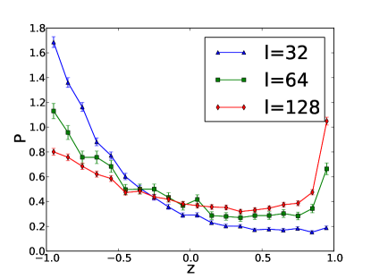
Figure 2: (Color Online) The distribution of scattering angles $\theta$. The horizontal axis is $z=\cos\theta$. The highest curve on the left is for $N=32$, the middle $N=64$, and the lowest $N=128$.

Assuming an athermal model, the temperature given by Eq. 2 is $k_{B}T=1/2$. The distribution of collision times is shown in Fig. 3 for $N=128$ (lower graph) and $N=64$ (upper graph.) The average time computed from this distribution, for $N=128$, is $210$. This is comparable but larger than the equilibrium relaxation time $t_{rel}$ seen for similar simulations of equilibrium systems. The latter was determined from measuring the time dependent autocorrelation function as has been described previously, see Ref. DeutschVacPRL , Fig. 3. This suggests that during the majority of these collisions, the system should be close to thermal equilibrium. There are two sets of data shown on each plot in Fig. 3. One where all scattering angles are included (triangles), the second only includes forward scattering, $z>0$ (squares). With only forward scattering, there is a prominent dip in the distribution at $t\approx 150$ ($N=128$.) For longer times, the two curves converge quite closely. The reason for this unusual small $t$ behavior will also be discussed below.

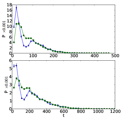
Figure 3: (Color Online) The distribution of collision times $t$ for a chain with $N=128$ (lower graph) and $N=64$ (upper graph), and the same distribution excluding those where the scattering angle is greater than $\pi/2$. The latter distribution has a sizable dip at $t\approx 150$ for $N=128$.

The distribution of final velocities is shown in Fig. 4(a). The smooth curve without error bars, is a fit to the form expected in the thermal limit, Eq. 11. Note that there is a much longer tail in the simulation data. If instead one excludes strong forward scattering, $z>0.9$, as shown in Fig. 4(b), the fit to the thermal distribution is much improved. The fit gives $\sigma_{x}=0.064$, where as the predicted value from Eq. 12, the thermal limit, is $0.044$. The distribution in Fig. 4(b) is still slightly too wide and this suggests that low final velocities are suppressed compared to the thermal prediction.

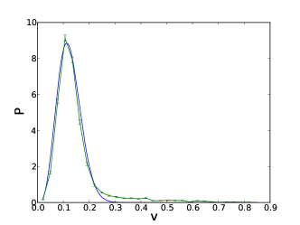
(a) (b)

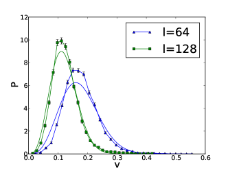
Figure 4: (Color Online) (a) The distribution of final collision speeds $v$ including all scattering angles and $N=128$. (b) The same distribution ignoring those where $\cos\theta<0.9$. For comparison the distribution for $L=64$ is also shown.

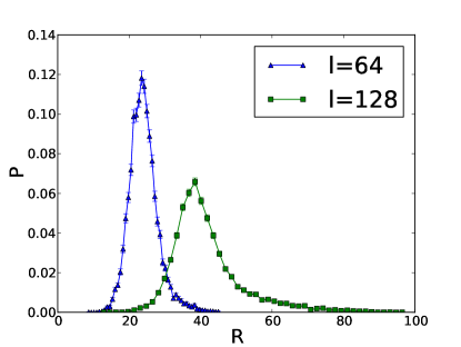
Figure 5: (Color Online) The distribution of the maximum end to end distances $R$, occurring during scattering for chains with $N=64$ and $128$.

The distribution of the maximum end to end distances $R$, occurring during scattering is shown in Fig. 5 for $N=64$ and $N=128$. There is typically substantial stretching that occurs during a collision. For comparison, statistics for the end to end distance $R_{e}$ for $N=128$ were calculated in thermal equilibrium for a total angular momentum of zero. The same chain has an rms end to end separation of $\sqrt{\langle R_{e}^{2}\rangle}=17.5$, However the maximum in Fig. 5 is at $R=38$ and has a significant tail stretching to past $R=90$. After the chains have separated, the stretching will disappear and tend towards their equilibrium values.

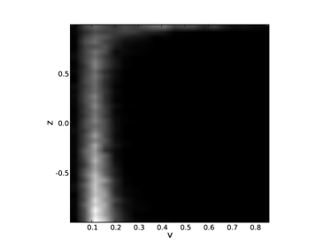
(a) (b)

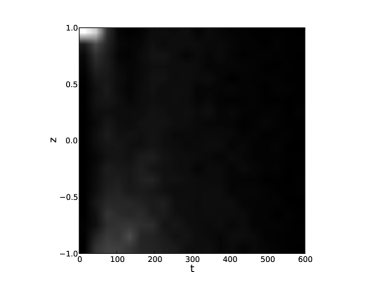
Figure 6: (a) The probability density as a function of final speed $v$, and the amount of deflection $z=\cos\theta$. (b) The probability density as a function of collision time $t$, and the amount of deflection $z=\cos\theta$.

To summarize what we have learned so far, collisions between self avoiding chains in a vacuum appear be quite close to what one would expect in the thermal limit. For the longest chain studied, $N=128$, the scattering is close to isotropic with the exception of a spike for strong forward scattering. The time that the chains remain in contact is typically longer than a relaxation time. The distribution of final speeds appears quite comparable to what one would expect from a thermal distribution except for collisions coming from strong forward scattering. Finally, at some point while the chains are in a collision, they are typically quite stretched.

From this it appears that these chain collisions are highly inelastic and they have properties close to that of collisions in the thermal limit. However there are some interesting deviations from this limit as was noted above. There appears to be a fraction of collision where the angle of scattering is very small. If these chains are excluded, then the collisions have statistics much closer to that of the thermal limit. A simple explanation for this would be that this sub-population of chains are not actually colliding. However their final velocities are substantially different from their initial ones, so this effect is clearly more subtle. By observing such strong forward scattering collisions it appears that their behavior can be understood as follows.

The dynamics of chains during collisions can be understood in terms of two factors, entanglement effects and transfer of momentum. During strong forward scattering collisions, it appears from visualizations, that the chains do strongly collide but only weakly entangle. Different parts of the chains come into contact and when they do, these parts collide very inelastically. That is, they do not bounce off one another but remain in contact for some length of time. Therefore momentum transfer between the chains is still inelastic. If two inelastic masses collide, even with unequal mass, their final velocity will still be along the same line as the initial velocities. Therefore all such inelastic collisions do not change the final direction. Because the chains have not entangled, they move past each other, but have not remained in contact long enough to thermalize. Their final directions are almost unchanged but their speeds have been substantially reduced due to momentum transfer.

The above observations can be seen by examining two dimensional distributions, for $N=128$ in Fig. 6. In Fig. 6(a), the distribution of collisions is binned in terms of final collision speed $v$, and $z$. One can see that for strong forward scattering, $z\approx 1$, there are a large number of collisions with final speeds much larger than the thermal velocity. In In Fig. 6(b), the distribution of collisions is binned as a function of collision time $t$ and $z$. Again for strong forward scattering, there is a high peak for atypically short times, indicating that the collisions are weaker than for other scattering angles. Therefore these strong forward scattering collisions are short and do not slow down the chains all the way to their thermal values.

The plots in Figs. 3 and 4 are obtainable from these two dimensional distributions. The enhancement in short time collision frequency seen in Fig. 3 for $z>0$ is therefore caused by the subset of strong forward scattering collisions, discussed above, that only collide for short times. All other collisions that more completely thermalize, usually remain in contact for longer times. The fact that there is a dip in the distribution of Fig. 3 when considering collisions with $z>0$ suggests that the quasi-thermal chains having $z>0$ have a peak in their collision time distribution at $t\approx 200$.

III Discussion

It is of interest to examine the scaling of collisions with $N$. The radius of gyration of a swollen chain $R\sim N^{\nu}$ with $\nu\approx 3/5$ in three dimensions. According to our assumption that the initial kinetic energy of the chains are zero, the probability that a monomer from chain A will collide with chain B is obtained by looking at the projection of the density of chain B into a two dimensional plane. The average density of this projection is proportional to the probability of a collision. The projected density is proportional to $N/R^{2}\sim N^{1-2\nu}\approx N^{-1/5}$. Therefore as $N\rightarrow\infty$ the probability that a given monomer in chain A will collide with chain B goes to zero. On the other hand, the total number of contact points in chain A is $N^{4/5}$. Therefore for large $N$ the molecules will suffer a collision but the above argument suggests that the number of monomers actually making contact will be a small fraction of the total.

If the amount of time that these points remain in contact is not long enough, the chains will pass each other at some reduced center of mass velocities. If the collisions of contact points are highly inelastic, only the speed of the chains, but not their direction, will change. Entanglements will change the above arguments considerably. Only one entanglement between two chains can cause their relative velocity to go to zero. For long enough chains, one would expect that entanglements would then dominate the collisions. However their effects usually only become dominant for chains larger than $N\approx 500$, as has been seen with the study of topological effects in flexible polymer rings DeutschRings

To understand the details of the dynamics of these collisions analytically is particularly difficult in light of the topological nature of the interactions and is beyond the scope of the present work. I would conjecture that the effects of entanglements will strongly suppress these forward scattering collisions for long enough chains.

If the chains are of different sizes, then their behavior will depend on their relative sizes. From the above discussion, the probability that a single monomer will collide with a polymer of $N_{1}$ links is $\propto N_{1}^{-1/5}$. Therefore if a second polymer is of length $N_{2}<N_{1}$, the probability of one collision is approximately $\propto N_{2}/N_{1}^{1/5}$. In other words, the second molecule is unlikely to collide if $N_{2}\ll N_{1}^{1/5}$. For chains of comparable sizes, the above results suggest that collisions will still be strongly inelastic and will also show behavior close to the thermal limit. The departure from this due to forward scattering will increase as the mass difference increases.

IV Conclusions

In this work, collisions between polymers in a vacuum have been examined. This is quite an unusual situation because collisions typically occur between much smaller molecules, and consequently new features of this situation are expected. The focus here is on chains where the initial relative center of mass velocity is so large that the initial internal thermal energy of the molecule can be ignored. This is an interesting limit to consider because for athermal chains, the magnitude of the initial velocity factors out.

Typically, in a collision of such long molecules, they remain in contact for long enough to be close to equilibrium so that they can be described by thermal averages. The final velocities and scattering angles, are close to such averages. However the main discrepancy with this description is due to a class of collisions that strongly forward scatter and remain in contact for a relatively short amount of time. This is evidence of strongly inelastic collisions of subsections of the chains. It is expected that for long enough chains, $N>500$ entanglement effects will diminish the frequency of these kinds of collisions.

In future work, it would be interesting to consider the case of chains with strong attractive forces as this may also be relevant to experiments and has interesting physical consequences. For example, chains at temperatures that are initially below the coil-globule transition will tend to stick together for low enough relative velocities. However beyond a threshold velocity, they would be expected to heat enough upon impact to become swollen and then separate from each other.

References

- (1) P.G. de Gennes “Scaling Concepts in Polymer Physics” Cornell University Press (1985).
- (2) F. Hillenkamp (Editor), J. Peter-Katalinic (eds.), “MALDI MS: A Practical Guide to Instrumentation, Methods and Applications” Wiley, (2007).
- (3) J.M. Deutsch, Phys. Rev. Lett. 99, 238301 (2007).
- (4) J.M. Deutsch, Phys. Rev. E 77, 051804 (2008).
- (5) A. Mossa, M. Pettini, and C. Clementi, Phys. Rev. E 74 041805 (2006).
- (6) M. P. Taylor, K. Isik and J. Luettmer-Strathmann, Phys. Rev. E 78, 051805 (2008).
- (7) J.M. Deutsch, Phys. Rev. E 81, 061804 (2010).
- (8) C.A. Barnes and N.H.L. Chiu, Intl J. Mass Spectrometry 279 170–175 (2009).
- (9) J. H. Moon, S. H. Yoon, and M. S. Kim, Bull. Korean Chem. Soc. 26 763 (2005).
- (10) F. Reif, “Fundamentals of statistical and thermal physics” McGraw-Hill (1965).
- (11) F. Reif, “Fundamentals of statistical and thermal physics” McGraw-Hill (1965), Chapter 7 section 12.
- (12) E. Fermi, J. Pasta, and S. Ulam, Studies of nonlinear problems (Los Alamos Document LA-1940, 1955).
- (13) For a review see G.P. Berman and F.M. Izrailev, Chaos 15, 015104 (2005) and references therein.
- (14) J.M. Deutsch, Phys. Rev. E 59, R2539 (1999).