Relationship between group sunspot number and Wolf sunspot number

Abstract

Continuous wavelet transform and cross-wavelet transform have been used to investigate the phase periodicity and synchrony of the monthly mean Wolf ($R_{z}$) and group ($R_{g}$) sunspot numbers during the period of June 1795 to December 1995. The Schwabe cycle is the only one common period in Rg and Rz, but it is not well-defined in case of cycles 5-7 of Rg and in case of cycles 5 and 6 of $R_{z}$. In fact, the Schwabe period is slightly different in $R_{g}$ and $R_{z}$ before cycle 12, but from cycle 12 onwards it is almost the same for the two time series. Asynchrony of the two time series is more obviously seen in cycles 5 and 6 than in the following cycles, and usually more obviously seen around the maximum time of a cycle than during the rest of the cycle. $R_{g}$ is found to fit $R_{z}$ better in both amplitudes and peak epoch during the minimum time time of a solar cycle than during the maximum time of the cycle, which should be caused by their different definition, and around the maximum time of a cycle, $R_{g}$ is usually less than $R_{z}$. Asynchrony of $R_{g}$ and $R_{z}$ should somewhat agree with different sunspot cycle characteristics exhibited by themselves.

1 Introduction

The single but most important index of solar activity has been the Zurich or Wolf sunspot number (the international sunspot number or the sunspot number) (Hathaway, Wilson, $\&$ Reichmann 2002; Hathaway 2010). For more than 100 years the Wolf sunspot number has served as the primary time series to define solar activity (Hoyt $\&$ Schatten 1998a, 1998b). It has been proven invaluable in studies of long-term variations in solar activity, especially as related to terrestrial climate (e.g., Eddy 1976; Hoyt $\&$ Schatten 1997; Li, Gao $\&$ Su 2005; ).

The sunspot number is defined as $R_{z}=k(10g+f)$, where $k$ is the normalization constant for a particular observer, $g$ is the number of sunspot groups, and $f$ the number of individual sunspots visible over the solar disk. In spite of the apparent arbitrary nature of this formula, it has been found to correlate extremely well with other, more physical measures of solar activity such as sunspot area, 10.7 cm radio flux, X-ray flare frequency, and magnetic flux (Hathaway, Wilson, $\&$ Reichmann 2002). Monthly values for $R_{z}$ are available from 1749 onward, but many of $R_{z}$ values between 1700 and 1850 are clearly based on inaccurate or missing data. Thus, these data are less accurate than more recent observations, and the $R_{z}$ values appear to be too large by 25 – 50$\%$ prior to 1882 (Hoyt $\&$ Schatten 1995a, b, c, d; Wilson 1998; Faria et al. 2004). A new parameter, the group sunspot number ($R_{g}$) was introduced by Hoyt $\&$ Schatten (1998a, 1998b) as an alternative to the sunspot number. It uses only the number of sunspot groups but is normalized to make it to agree with the Zurich sunspot number. With this normalization the group sunspot number is given by $R_{g}={{12.08}\over{N}}\sum_{i=1}^{N}(k_{i}g_{i})$, where $k_{i}$ is the correction factor for observer $i$, $g_{i}$ is the number of sunspot groups observed by observer $i$, and $N$ the number of observers used to form the daily value. The group sunspot number is more self-consistent and less noisy than the sunspot number. Daily, monthly, and annual observations were determined during the period of the years 1610 – 1995. The Wolf and group sunspot numbers are the longest direct instrumental records of solar activity (Rigozo et al. 2001; Kane 2002; Ogurtsov et al. 2002; Echer et al. 2005). Hathaway, Wilson, $\&$ Reichmann (2002) examined the group sunspot number and compared the sunspot cycle characteristics it exhibits to those exhibited by the Wolf sunspot number. They found that the Wolf sunspot number continues to be valuable in capturing characteristics of the recent cycles that are not quite as well-reflected in the group number, and the group sunspot number is valuable for capturing the behavior in the earliest cycles that help to reveal long-term behavior. Ogurtsov et al. (2002) used the yearly Wolf sunspot number and the yearly group sunspot number to study long periods of solar activity through Morlet wavelet analysis and Fourier analysis. Faria et al. (2004) compared the spectral features of the yearly group sunspot number and the yearly Wolf sunspot number with the use of multitaper analysis and Morlet wavelet analysis. Li et al. (2005) investigated the Schwabe and Gleissberg periods in the Wolf sunspot number and the group sunspot number. However, no one has investigated phase relationship between them up to now, and the difference between the two caused by their different definition has not yet been paid enough attention.

According to the modern point of view, synchronization is an universal concept in nonlinear sciences (Pikovsky, Rosenblum $\&$ Kurths 2001; Maraun $\&$ Kurths 2004; Romano et al. 2005). In the present study, we will use the cross-wavelet transform method to study phase relation between the monthly mean group sunspot number and the monthly mean sunspot number and investigate the influence of their different definition on the relation between them.

2 Wavelet analyses of the monthly mean Wolf and group sunspot numbers

2.1 Data

The continuous time series of the monthly mean sunspot number ($R_{z}$) is available from January 1749, and the continuous time series of the monthly mean group sunspot number ($R_{g}$) is available from June 1795 to December 1995. Figure 1 shows both $R_{g}$ and $R_{z}$ from June 1795 to December 1995, which are both downloaded from the NOAA’s web site. These two kinds of data are used to investigate the phase relationship between them. As the figure shows, $R_{g}$ obviously differs from $R_{z}$ around the maximum time of a cycle, implying that they should be asynchronous.

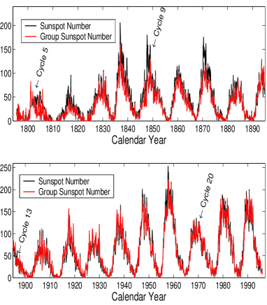
Figure 1: The monthly mean group sunspot number (the black line) and the monthly mean sunspot number (the red line) from June 1795 to December 1995.

2.2 Continuous wavelet transform

Wavelet analysis involves a transform from an one-dimensional time-series to a diffuse two-dimensional time-frequency image for detecting the localized and (pseudo-) periodic fluctuations by using the limited time span of the data (Torrence $\&$ Compo 1998; Li et al. 2005). Here the Morlet continuous wavelet transform (CWT) is used with its dimensionless frequency $\omega_{0}=6$. Figure 2 shows the continuous wavelet power spectra of $R_{g}$ and $R_{z}$. There are evidently common features in the wavelet power spectra of the two time series. The both have a large-scale periodicity (about 11 years, namely the Schwabe cycle) of the highest power, above the 95$\%$ confidence level. However, the Schwabe cycle does not significantly exist in cycles 5 to 7 for $R_{g}$ and in cycles 5 and 6 for $R_{z}$.

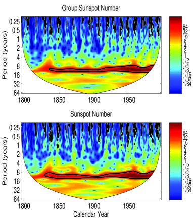
Figure 2: The continuous wavelet power spectra of the monthly mean group sunspot number (top) and the monthly mean sunspot number (bottom). The thick black contours indicate the 95$\%$ confidence level, and the white region below the thin solid line indicates the cone of influence (COI) where edge effects might distort the picture (for details, see Torrence $\&$ Compo 1998).

Figure 3 displays the period length of the Schwabe cycle varying with time respectively for the two time series. At a certain time point, the Schwabe period (scale) of $R_{g}$ (or $R_{z}$) has the highest spectral power among all considered time scales in its local wavelet power spectrum, thus the Schwabe period length is determined at a certain time point. As the figure shows, the Schwabe period for $R_{g}$ and $R_{z}$ actually differs from each other before cycle 12, but from cycle 12 onwards it is almost the same for the two time series. If period (frequency) of two time series is different, the two are asynchronous. The differences of the Schwabe cycle length for the two time series should lead to a phase asynchrony between them.

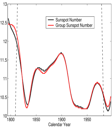
Figure 3: The period length of the Schwabe cycle for the monthly mean group sunspot number (the red line) and that for the monthly mean sunspot number (the black solid line). The two dashed lines indicate the COI.

2.3 Cross-wavelet transform

Cross-wavelet transform (XWT) is an extension of wavelet transforms to expose the common power and relative phase between two time series in time-frequency space (Li et al 2009 and references therein). The cross – wavelet transform of two time series $X$ and $Y$ is defined as $W^{XY}=W^{X}W^{Y\ast}$, where $\ast$ denotes complex conjugation and $W^{X}$ and $W^{Y}$ are the continuous wavelet transforms of the individual time series (Grinsted et al. 2004). The complex argument $arg(W^{XY})$ can be interpreted as a local relative phase between $X$ and $Y$ in time-frequency space, namely the phase angle difference of $X$ and $Y$. We employ the codes provided by Grinsted et al. (2004) to get the XWT of the two time series in order to investigate their phase relationship. Figure 4 shows the XWT of the two time series. The two time series are in phase in the area, namely about an 11 yr periodic belt, with significant common power, because all arrows point right in the area.

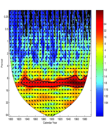
Figure 4: The cross wavelet transform of the monthly mean group sunspot number and the monthly mean sunspot number. The thick black contours indicate the $95\%$ confidence level, and the region below the thin line indicates the COI. The relative phase relationship is shown as arrows with in-phase pointing right, anti-phase pointing left, and the former leading the latter by $90^{\circ}$ pointing straight down.

The real and imaginary parts of a wavelet power spectrum are considered separately, and the phase angle at any point of the wavelet power spectrum can be obtained through its complex spectral amplitude (Li et al. 2009). Figure 5 shows the phase angle (argument) of the complex cross-wavelet amplitudes varying with frequency and time. It is the relative phase of the two time series. The results shown in the figure clearly indicate that the relative phases coherently fluctuate within a rather large range of frequencies, which correspond to the period scales of larger than 4 years. At smaller scales, there are no regular oscillatory patterns in the corresponding frequency bands, and the high-frequency components demonstrate a noisy behavior with strong phase mixing.

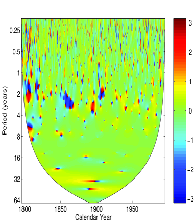
Figure 5: The relative phase angles (arguments) of the complex cross-wavelet amplitudes varying with frequency and time. The thin solid line indicates the COI.

Based on Figure 5, we calculate the averages of relative phase angles over all scales for all time points of the considered interval, which are displayed in Figure 6. Their corresponding standard deviations are also calculated and shown in Figure 7. As the two figures show, the relative phase of the two time series fluctuates within larger amplitudes in cycles 5 and 6 than that in all the following cycles does, and it fluctuates within larger amplitudes usually around the maximum time of a cycle than around the minimum time of the cycle. Asynchrony of the two time series is thus more obviously seen in cycles 5 and 6 than in the following cycles, and usually more obviously seen around the maximum time of a cycle than during the rest of the cycle.

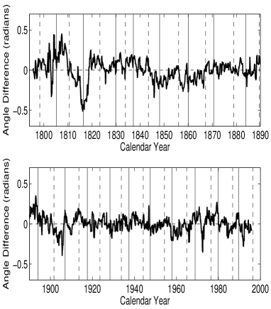
Figure 6: The average (the thick solid line) of relative phases over all period scales shown in Figure 5 varying with time. The dashed (solid) vertical lines show the minimum (maximum) times of cycles.

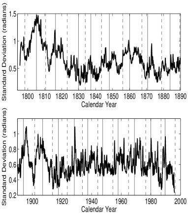
Figure 7: The corresponding standard deviation (the thick line) of the average of relative phases shown in Figure 6. The dashed (solid) vertical lines show the minimum (maximum) times of cycles.

For the two time series, the mean relative phases are shown in Figure 8 in dependence on the considered frequencies. The corresponding standard deviations have been calculated as well and are given in the second panel of the figure. As the figure shows, the relative phases obviously coherently fluctuate within time scales of about 8 to 13 years (and even within 8 to 25 years), where their relative phases are within $\pm 0.2$ radian, and their standard deviations are less than 0.5 radian. Although the relative phases are always negative within time scales of about 8 to 13 years, seemingly indicating $R_{z}$ leading $R_{g}$, the corresponding standard deviations are so large that we could not think $R_{z}$ leading $R_{g}$. At time scales of less than 8 years, the relative phase angles violently fluctuate and their standard deviations are very large. The relative phase angles increase after time scales of larger than 25 years, and their standard deviations also increase.

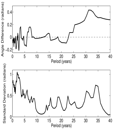
Figure 8: Angle difference (the relative phase) of the XWT power spectrum of of the monthly mean group sunspot number and the monthly mean sunspot number as a function of periods (the top panel) and its corresponding standard deviations (the bottom panel). Positive values should be interpreted as the monthly mean group sunspot number leading the monthly mean sunspot number.

Taking very small or very large reference time scales into account should lead to non-coherent behavior of the phase variables assigned to $R_{g}$ and $R_{z}$. In the following, we therefore focus attentions on periodicities in the coherent range around the Schwabe cycle as the reference time scales. Because the high-frequency components of $R_{g}$ and $R_{z}$ are filtered out in such a case, the resulting phases are well-defined and may be used to study the varying relationship between $R_{g}$ and $R_{z}$. Based on Figure 5, we calculate the averages of relative phase angles over scales of 8 to 13 years for all time points of the considered interval, which are displayed in Figure 9. Their corresponding standard deviations are also calculated and shown in the figure. As the figure indicates, for all cycles except cycles 5 and 6, the mean relative phase angles are very small (within $\pm 0.35$ radian), fluctuating around the value of zero, and the standard deviations are small (less than 0.5 radian). It is the low-frequency components of hemispheric flare activity in period scales around the Schwabe cycle that are responsible for the strong phase synchronization. Based on Figure 5, we calculate the averages of relative phase angles over scales of 8 to 25 years for all time points of the considered interval, which are also displayed in Figure 9. Their corresponding standard deviations are calculated and shown in the figure. As the figure indicates, for all cycles except cycles 5 and 6, the mean relative phase angles are very small (even within $\pm 0.2$ radian), fluctuating around the value of zero, and the standard deviations are small (less than 0.7 radian). For cycles 5 and 6, there are no coherent frequencies.

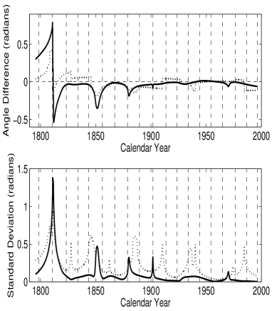
Figure 9: The average of relative phases over the period scales respectively of 8 to 13 years (the solid line) and of 8 to 25 years (the dotted line) varying with time (the top panel), and its corresponding standard deviation (the lower panel) with the XWT method used. Solid (dotted) line corresponds to solid (dotted) line in the two panels.

3 Influence of their different definition on the relation between them

As we know, during the minimum time of a cycle a group of sunspots has only one sunspot in the most cases or two sometimes, thus $(10g+f)/g\approx 11$. However, during the maximum time of a cycle a group of sunspots has one to two sunspots sometimes, or several (or even more) sunspots sometimes, thus $(10g+f)/g$ is larger than 11 and believed even usually larger than 12.08 (the normalization constant in the definition of $R_{g}$). Therefore, there should certainly exist difference between the two caused by their different definition. The median value of $R_{g}$ is about 46.4, and $R_{g}$ is divided into two group: in one (G1) $R_{g}$ is less than, and in the other (G2) $R_{g}$ is larger than the median. A linear fit is done for each of the two groups, which is shown in Figure 10. The fitting line is $R_{g}=1.5+0.897\times R_{z}$ with the correlation coefficient of 0.965 for the group $G1$, and $R_{g}=8.2+0.883\times R_{z}$ with the correlation coefficient of 0.962 for the group $G2$. As the figure shows, the fitting line is very close to the straight line $R_{g}=R_{z}$ for $G1$. However, for $G2$ the fitting line is generally below the straight line $R_{g}=R_{z}$, and the deviation between the two increases with the increase of $R_{g}$. Conclusively, $R_{g}$ matches $R_{z}$ very well around the minimum time of a cycle, but during the maximum time of a cycle it seems usually less than $R_{z}$. $R_{g}$ and $R_{z}$ are doomed by their different definition to present different relationship between them at different stage of a cycle.

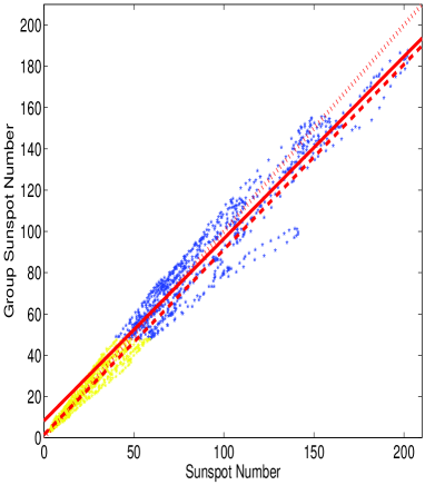
Figure 10: Relationship between $R_{g}$ and $R_{z}$. $R_{g}$ is divided into two group: in one (G1) $R_{g}$ is less than its median (the yellow asterisks), and in the other (G2) $R_{g}$ is larger than the median (the blue asterisks). A linear fit is done for each of the two groups (the dashed line is for G1, and the solid for G2). The dotted line is the line of that $R_{g}=R_{z}$.

The maximum value of a sunspot cycle is an important parameter to characterize the sunspot cycle. Figure 11 displays the maximum values of the Wolf sunspot number and the group sunspot number in the modern cycles (cycles 10 to 22). The maximum value of the sunspot number in a cycle is usually larger than that of the group sunspot number (cycles 10 to 12 and 18 to 22) or very close to the corresponding one of the group sunspot number (cycles 13 to 17), confirming the aforementioned result. The average of the sunspot number maxima over cycles 10 to 22 is 135.5, and the average of the group sunspot number maxima is 132.0, slightly less than the former. We also show in the figure the difference between the maximum time of the sunspot number and the group sunspot number in a cycle for the modern cycles. In 9 of the total 13 cycles, the difference is obvious, indicating asynchrony of $R_{g}$ and $R_{z}$.

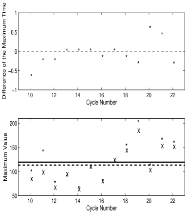
Figure 11: The top panel: difference (asterisks) between the maximum time of the sunspot number and the group sunspot number in a cycle. The dashed line shows no differences. The bottom panel: the maximum values of the sunspot number (asterisks) and the group sunspot number (crosses). The solid line shows the average (135.5) of the sunspot number maxima over cycles 10 to 22, and the dashed, the average (132.0) of the group sunspot number maxima.

4 Conclusions and discussions

In the present study, the continuous wavelet transform and the cross-wavelet transform have been proposed to investigate the phase synchrony of the monthly mean Wolf and group sunspot numbers, the longest direct instrumental records of solar activity, and the data used here span from June 1795 to December 1995.

The continuous wavelet transforms of the two time series show that the 11-year Schwabe cycle is the only one period of statistical significance for the two time series, and it is 10.7 years. However, in cycles 5 to 7 the Schwabe cycle does not significantly exist for $R_{g}$, and in cycles 5 and 6 for $R_{z}$.

The Schwabe period for $R_{g}$ and $R_{z}$ actually slightly differs from each other before cycle 12, but from cycle 12 onwards it is almost the same for the two time series. If period (frequency) of two time series is different, the two are asynchronous. The slight differences of the Schwabe cycle length for the two time series should lead to a slight phase asynchrony between them.

The cross-wavelet transform (XWT) of the two time series shows that there is an area, locating at the Schwabe-cycle periodic belt, where the two time series are approximately in phase. Through the XWT analysis, the relative phase angles are found to coherently fluctuate in a small angle range only within a range of frequencies which corresponds to time scales around the Schwabe cycle, and even within time scales of about 8 to 25 years. The high-frequency components demonstrate a noisy behavior with strong phase mixing. It is the low-frequency components of $R_{g}$ and $R_{z}$ in period scales around the Schwabe cycle that are responsible for the strong phase synchronization. Taking very small or very large reference time scales into account should lead to non-coherent behavior of the phase variables assigned to $R_{g}$ and $R_{z}$ at the respective scales. Asynchrony of the two time series is found more obvious in cycles 5 and 6 than in the following cycles, and more obvious usually around the maximum time of a cycle than during the minimum time of the cycle, indicating that $R_{g}$ should fit $R_{z}$ better in both amplitudes and peak epoch during the minimum time time of a solar cycle than during the maximum time of the cycle. As we know, during the minimum time of a cycle a group of sunspots has only one sunspot generally or two sometimes, thus $(10g+f)/g\approx 11$. However, during the maximum time of a cycle a group of sunspots has one to two sunspots sometimes, or several (or even more) sunspots sometimes, thus $(10g+f)/g$ is larger than 11 and believed even usually larger than 12.08 (the normalization constant in the definition of $R_{g}$), and further it is scattered within a wider range than during the minimum of the cycle. $R_{g}$ is destined to match $R_{z}$ better during the minimum time than during the maximum time of a cycle, making the two more obviously asynchronous during the maximum time than during the minimum time of a cycle, and further, $R_{g}$ is usually less than $R_{z}$ around the maximum time of a cycle.

Somewhat in agreement with the more obvious asynchrony of the two during the maximum times than during the the corresponding minimum times of solar cycles, the “Waldmeier Effect” - the anti-correlation between cycle amplitude and the elapsed time between minimum and maximum of a cycle - is much more apparent in the Zurich numbers; the “Amplitude-Period Effect” - the anti-correlation between cycle amplitude and the length of the previous cycle from minimum to minimum - is also much more apparent in the Zurich numbers; the “Even-Odd Effect” - in which odd-numbered cycles are larger than their even-numbered precursors - is somewhat stronger in the Group numbers but with a tighter relationship in the Zurich numbers; the ‘Secular Trend’ - the increase in cycle amplitudes since the Maunder Minimum - is much stronger in Group numbers (Hathaway, Wilson $\&$ Reichmann 2002). Due to that $R_{g}$ matches $R_{z}$ worse during the maximum time than during the minimum time of a cycle, they exhibit the above different sunspot cycle characteristics and more obvious asynchrony during the maximum time of the cycle.

Sunspot number, group sunspot number and sunspot area are widely and frequently utilized in astronomy and Earth science to embody long-term variations of solar activity. However, reviewed from the phase relationship between each two of the three, they are slightly asynchronous in phase, although they are coherent in the low-frequency components corresponding to the period scales around the Schwabe cycle, this is inferred the main reason why “the Zurich numbers follow the 10.7-cm radio flux and total sunspot area measurements only slightly better than the Group numbers” (Hathaway, Wilson $\&$ Reichmann 2002). Which one of the three can be served as the best primary time series to define solar activity? it is an open question, and careful attention should be paid.

- [1] Echer, E., Gonzalez, W.D., Guarnieri, F.L., Lago, A.Dal, Vieira, L.E.A.: 2005, Advances in Space Research 35, 855
- [2] Eddy, J.A.: 1976, Science 192, 1189
- [3] Faria, H.H., Echer, E., Rigozo, N.R., Viera, L.E.A.: 2004, Sol. Phys. 223, 305
- [4] Grinsted, A., Moore, J.C., Jevrejeva, S.: 2004, Nonlinear. Proc. Geophys. 11, 561
- [5] Hathaway, D.H.: 2010, Living Reviews in Solar Physics 7, 1
- [6] Hathaway, D.H., Wilson, R.M., Reichmann, E.J.: 2002, Sol. Phys. 211, 357
- [7] Hoyt, D.V., Schatten, K.H.: 1995a, Sol. Phys. 160, 371
- [8] Hoyt, D.V., Schatten, K.H.: 1995b, Sol. Phys. 160, 379
- [9] Hoyt, D.V., Schatten, K.H.: 1995c, Sol. Phys. 160, 387
- [10] Hoyt, D.V., Schatten, K.H.: 1995d, Sol. Phys. 160, 393
- [11] Hoyt, D.V., Schatten, K.H.: 1997, The Role of Sun in Climate Changes (New York: Oxford University Press)
- [12] Hoyt, D.V., Schatten, K.H.: 1998a, Sol. Phys. 179, 189
- [13] Hoyt, D.V., Schatten, K.H.: 1998b, Sol. Phys. 181, 491
- [14] Kane, R.P.: 2002, Sol. Phys. 205, 383
- [15] Li, K.J., Gao, P.X., Su, T.W.: 2005, Sol. Phys. 229, 181
- [16] Li, K.J., Gao, P.X., Zhan, L.S., Shi, J.X., Zhu, W.W.: 2010, MNRAS, 401, 342
- [17] Maraun, D., Kurths, J.: 2004, Nonlinear Proc. Geophys. 11, 505
- [18] Ogurtsov, M.G., Nagovitsyn, Yu.A., Kocharov, G.E., Jungner, H.: 2002, Sol. Phys. 211, 371
- [19] Pikovsky, A., Rosenblum, M., Kurths, J.: 2001, Synchronization: A Universal Concept in Nonlinear Science (Cambridge: Cambridge University Press)
- [20] Rigozo, N.R., Echer, E., Vieira, L.E.A., Nordemann, D.J.R.: 2001, Sol. Phys. 203, 179
- [21] Romano, M.C., Thiel, M., Kurths, J., Kiss, I.Z., Hudson, J.L.: 2005, Europhys. Lett. 71, 466.
- [22] Torrence, C., Compo, G.P.: 1998, Bull. Amer. Meteor. Soc. 79, 61
- [23] Wilson R.M.: 1998, Sol. Phys. 182, 217