Spherical single-roll dynamos at large magnetic Reynolds numbers

Abstract

This paper concerns kinematic helical dynamos in a spherical fluid body surrounded by an insulator. In particular, we examine their behaviour in the regime of large magnetic Reynolds number $R_{\text{m}}$, for which dynamo action is usually concentrated upon a simple resonant stream-surface. The dynamo eigensolutions are computed numerically for two representative single-roll flows using a compact spherical harmonic decomposition and fourth-order finite-differences in radius. These solutions are then compared with the growth rates and eigenfunctions of the Gilbert and Ponty (2000) large $R_{\text{m}}$ asymptotic theory. We find good agreement between the growth rates when $R_{\text{m}}\!>\!10^{4}$, and between the eigenfunctions when $R_{\text{m}}\!>\!10^{5}$.

1 Introduction

We consider a class of kinematic dynamos in which the magnetic field $\mathbf{B}$ is generated by the steady helical motion $\mathbf{v}$ of an incompressible, electrically-conducting fluid. Helical flows constitute some of the simplest and most efficient mechanisms for the excitation of a seed magnetic field, as witnessed in numerical simulation and exploited by laboratory experiments (Gailitis et al. 1987, Dudley & James 1989, Forest et al. 2002, Moss 2008, for example). Such flows are also widespread in astrophysical fluid bodies, such as jets, the convection zones of stars and, possibly, liquid planetary cores, where they might appear as a slow meridional circulation (Giles et al. 1997, Gough and McIntyre 1998, Olson et al. 1999, Haber et al. 2002, Hartigan et al. 2005).

By far the simplest helical flow is the Ponomarenko dynamo (Ponamerenko 1973), which consists of a solid electrically-conducting cylinder of finite radius rotating with constant angular velocity $\Omega$ and translating with a constant axial velocity $V$, while its rigid (electrically-conducting) exterior remains at rest. The dynamo loop in this case comprises (a) generation of azimuthal magnetic field from radial magnetic field by the discontinuity in the rotation (the ‘omega effect’), and (b) reciprocal generation of radial field from azimuthal field by magnetic diffusion. Note that the additional longitudinal shearing component $V$ is crucial, as it draws apart oppositely directed field lines and prevents flux expulsion. Ponomarenko (1973) determined the magnetic field in this case analytically, showing that the field is concentrated at the velocity discontinuity on the cylinder boundary. Helical dynamos with non-uniform $V$ and $\Omega$ and arbitrary cross-section, such as in a conducting fluid, are naturally more complicated (but see the exact steady solutions of Lortz 1968, and Chen & Milovich 1984). Nevertheless, they share the same dynamo ingredients: differential rotation and magnetic diffusion. These ingredients are especially conspicuous at very large magnetic Reynolds number $R_{\text{m}}$, a regime which can be probed successfully with asymptotic theory (Ruzmaikin et al. 1988, Gilbert 1988, Gilbert & Ponty 2000, hereafter GP). In such models the importance of diffusion, in particular, is evident from the localisation of potentially growing dynamo modes upon their critical surfaces, where the modes are nearly convected by the flow. It is upon these surfaces that the modes exhibit the small-scale variation necessary for magnetic diffusion to work effectively and replenish radial magnetic field. Not every stream-surface can support a mode, but a ‘resonance condition’ selects the critical surface (or surfaces) upon which dynamo action can occur.

The asymptotics of helical dynamos in an infinite cylinder have been generalised to helical dynamos in a sphere (GP). A spherical single-roll dynamo can be portrayed as a cylindrical helical flow with its two ends joined, bent into a donut, and deformed to fill a spherical ‘container’. The theory predicts that at large $R_{\text{m}}$ the dominant mechanism of field generation is of Ponamarenko type and, indeed, that the same asymptotic scalings hold. However, full numerical studies of the dynamo problem in spheres have mostly tested small or intermediate $R_{\text{m}}$, primarily to establish the critical $R_{\text{m}}$ necessary for dynamo action (Dudley & James 1989, Forest et al. 2002, Moss 2008). The very large $R_{\text{m}}$ regime has not received the same attention, partly because it remains a challenging numerical task. Consequently, the GP asymptotic theory has not yet been numerically confirmed. This is the main project of our paper

We undertake an analysis of single-roll helical dynamos in a sphere, surrounded by an insulator, at very large magnetic Reynolds numbers. This is accomplished numerically by the solution of the magnetic induction equation with suitable boundary conditions for two representative single-roll flows. The method of solution is presented in Ivers and Phillips (2003, 2008) and consists of approximating the problem as a large-scale algebraic eigenvalue equation. The growth rates and eigenfunctions so obtained are subsequently compared with the predictions of the GP asymptotic theory. We find excellent agreement in the regime $R_{\text{m}}>10^{4}$ for the growth rates and angular frequency, and good agreement for the magnetic field structure when $R_{\text{m}}>10^{5}$. In particular, the magnetic field structure clearly localises upon a specific stream-surface, in contrast to intermediate $R_{\text{m}}$ where the field is somewhat disordered. This confirms that spherical single-roll dynamos are indeed of the Ponamerenko type: no other growing modes were discovered. This is a point that can deepen our understanding of spherical dynamos more generally and aid the analysis of more complex spherical flows. In particular, it is an entry point into the study of multiple rolls, whose magnetic field generation will also be influenced by the Gailitis dynamo mechanism (Gailitis 1970, 1993, 1995, Moss 2006).

The layout of the paper is as follows. In Section 2, the formal dynamo problem is stated — its governing equations, parameters, and boundary conditions — and the two flows we examine are presented. A brief summary of the GP asymptotic results at large $R_{\text{m}}$ follows in Section 3, while their derivation is given in Appendix A, in the Supplemental Material, alongside a method to obtain higher order terms. Our results and a comparison of the two approaches are given in Section 4, and conclusions drawn in Section 5.

2 Governing equations and setup

2.1 Problem formulation

Consider a sphere of conducting fluid $V$ with radius $a$ and uniform magnetic diffusivity $\eta$ surrounded by an insulator $V^{c}$. Suppose that the fluid is undergoing time-steady incompressible motions according to the velocity $\mathbf{v}$. Consequently, the magnetic field in the conducting fluid is governed by the non-dimensionalised induction equation,

$$\partial_{\tau}\mathbf{B}=\nabla^{2}\mathbf{B}+R_{\text{m}}\nabla\times(\mathbf{v}\times\mathbf{B})$$ (2.1)

where the magnetic Reynolds number $R_{\text{m}}=\mathcal{V}a/\eta$ is defined in terms of a typical velocity $\mathcal{V}$, the radius $a$, and $\eta$. The time $\tau$ is scaled on the magnetic diffusion time $\mathcal{L}^{2}/\eta$ and space by $a$. The magnetic field $\mathbf{B}$ is solenoidal everywhere,

$$\nabla\cdot\mathbf{B}=0\,.$$ (2.2)

Because the flow is steady, the magnetic field can be expressed as a linear superposition of time-separable solutions of the form

$$\mathbf{B}(\mathbf{r},\tau)=\mathbf{B}(\mathbf{r})e^{\lambda\tau}\,,$$ (2.3)

possibly with polynomial factors of time in degenerate cases. In addition, we must supply suitable boundary conditions

$$[\mathbf{B}]_{\Sigma}=\mathbf{0}\,,\qquad\nabla\times\mathbf{B}=\mathbf{0}\quad\text{in $V^{c}$,}\qquad\mathbf{B}\to\mathbf{0}\quad\text{as $r\to\infty$,}$$ (2.4)

where $\Sigma$ is the surface of the sphere. This leads to an eigenvalue problem for the (complex) growth rate $\lambda$ and the associated eigenfunction. For a given flow $\mathbf{v}$, the growth rate $\lambda$ is a function of the magnetic Reynolds number $R_{\text{m}}$. When $\operatorname{Re}\lambda>0$, the flow acts as a kinematic dynamo, i.e. the non-magnetic state $\mathbf{B}=\mathbf{0}$ is unstable to magnetic perturbations.

2.2 Representation of the helical flow

We use spherical coordinates whereby the radius, polar angle, and azimuthal angle are denoted by $r$, $\theta$, and $\phi$, with their accompanying unit vectors given by $\mathbf{1}_{r}$, $\mathbf{1}_{\theta}$, and $\mathbf{1}_{\phi}$, respectively. An axisymmetric single-roll helical flows may be represented by

$$\mathbf{v}=\sigma\,\mathbf{V}_{\text{m}}+W(r,\theta)\,r\,\sin\theta\,\mathbf{1}_{\phi},$$ (2.5)

where $\mathbf{V}_{\text{m}}$ is the (scaled) meridional velocity, $W$ is the azimuthal angular speed, and $\sigma$ is a parameter measuring the relative strengths of the meridional and azimuthal motion. The meridional flow $\mathbf{V}_{\text{m}}$ can be written in terms of a stream function $\Psi$ by

$$\mathbf{V}_{\text{m}}=-\frac{\partial_{\theta}\Psi}{r^{2}\sin\theta}\mathbf{1}_{r}+\frac{\partial_{r}\Psi}{r\sin\theta}\mathbf{1}_{\theta}=\nabla\phi\times\nabla\Psi=-\nabla\times\frac{\Psi}{r\sin\theta}\mathbf{1}_{\phi}\,.$$ (2.6)

The streamlines of $\mathbf{V}_{\text{m}}$ in a meridional plane are the level contours of $\Psi$ and circle a local minimum (maximum) of $\Psi$ in the clockwise (counter-clockwise) direction. We also introduce the ‘unscaled’ meridional velocity $\mathbf{v}_{\text{m}}=\sigma\mathbf{V}_{\text{m}}$ and stream function $\psi=\sigma\Psi$, which are more convenient when describing the asymptotic theory.

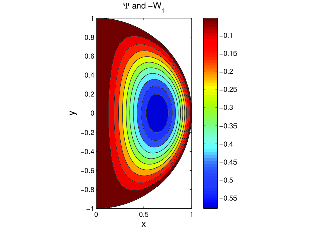
Figure 1: A representation of the meridional circulation shared by both flow 1 and 2. The coloured isocontours of the meridional stream function $\Psi$ are plotted. The negative of this function is also the azimuthal angular speed of flow 1, as $W_{1}=-\Psi$.

In this paper, we examine two representative single-roll flows, $\mathbf{v}_{1}$ and $\mathbf{v}_{2}$. The two flows share the same meridional velocity $\mathbf{V}_{\text{m}}$ but differ in the azimuthal component $W\,r\,\sin\theta$. We set the stream function $\Psi$ according to

$$\Psi(r,\theta)=-r\sin\pi r\sin^{2}\theta\,,$$ (2.7)

but set

$$W_{1}=r\sin\pi r\,\sin^{2}\theta\,,\qquad W_{2}=\frac{\sin\pi r}{r}\,.$$ (2.8)

Flow 1 therefore possesses the restricted form $W_{1}=W_{1}(\Psi)=-\Psi$, while flow 2 has a more general form. The restricted form of the local angular velocity simplifies the asymptotic theory substantially.

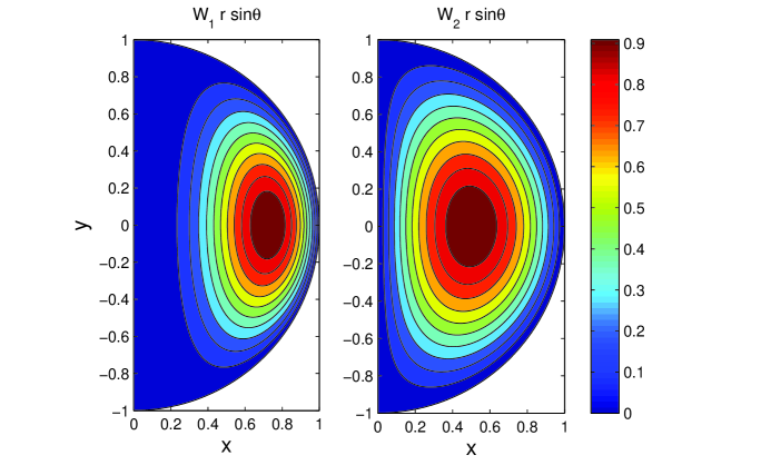
Figure 2: A representation of the two azimuthal flows considered. The left panel shows the azimuthal velocity of flow 1, $W_{1}\,r\sin\theta$, while the right panel shows that of flow 2, $W_{2}\,r\sin\theta$.

In Figs 1 and 2 the two flows are represented. Figure 1 shows the isocontours of $\Psi$, the meridional stream function common to both flows. As the figure indicates, fluid circulates in a clockwise direction around a central stagnation point located at $r\approx 0.646$. In the case of flow 1, for which $W_{1}=-\Psi$, the isocontours of the azimuthal rotation coincide with the isocontours of the meridional rotation. Therefore a fluid element upon a given streamsurface will not only circulate at a constant speed in the meridional plane it will also travel at a constant angular speed in the azimuthal direction. It is then easier to find flow trajectories that form closed loops.

This is not the case for the more complicated flow 2, whose azimuthal angular speed exhibits a purely radial profile. Thus surfaces of constant rotation are spherical shells. This means a fluid element in flow 2 will experience different azimuthal angular velocities as it traverses a meridional streamline. The actual azimuthal velocities, $Wr\sin\theta$, of both flows are plotted in Fig. 2.

The full numerical method we employ requires that the velocities are split into toroidal and poloidal components and expanded in spherical harmonics:

$$\mathbf{v}=\sum_{m,n}\mathbf{t}_{n}^{m}\,+\,\sum_{m,n}\mathbf{s}_{n}^{m}\,,$$

where the toroidal components are given by $\mathbf{t}_{n}^{m}=\nabla\times(t_{n}^{m}Y_{n}^{m}\mathbf{r})$ and the poloidal components by $\mathbf{s}_{n}^{m}=\nabla\times\nabla\times(s_{n}^{m}Y_{n}^{m}\mathbf{r})$, where $Y_{n}^{m}$ is a spherical harmonic (see Ivers & Phillips 2003, 2008).

Flow 1 has the poloidal-toroidal spectral decomposition $\mathbf{v}_{1}=\sigma\,\mathbf{s}_{1}^{0}+\mathbf{t}_{1}^{0}+\mathbf{t}_{3}^{0}$, in which the radial functions are

$$s_{1}^{0}=\frac{\sin\pi r}{\sqrt{3}}\,,\qquad t_{1}^{0}=-\frac{4}{5\sqrt{3}}\,r^{2}\sin\pi r\,,\qquad t_{3}^{0}=\frac{2}{15\sqrt{7}}\,r^{2}\sin\pi r\,,$$ (2.9)

and the spherical harmonics are $Y_{1}^{0}=\sqrt{3}\,\cos\theta$ and $Y_{3}^{0}=\tfrac{1}{2}\sqrt{7}\,\cos\theta(5\cos^{2}\theta-3)$.

The second flow $\mathbf{v}_{2}$ is the single-roll flow of Dudley & James (1989). This flow has the poloidal-toroidal spectral form $\mathbf{v}_{2}=\sigma\,\mathbf{s}_{1}^{0}+\mathbf{t}_{1}^{0}$, where

$$s_{1}^{0}=\frac{\sin\pi r}{\sqrt{3}}\,,\qquad t_{1}^{0}=\sin\pi r\,.$$ (2.10)

Although $\mathbf{v}_{1}$ has the simpler restricted form of the local angular velocity, its spherical harmonic representation is actually more complicated than $\mathbf{v}_{2}$.

3 The GP asymptotic theory

This section summarises the main features and results of the GP asymptotic theory, undertaken at large $R_{\text{m}}$. Here we give, without proof, the leading order terms for the growth rates at $\mathcal{O}(R_{\text{m}}^{-1/2})$ and the leading order contribution to the magnetic eigenfunction. The derivations of these expressions are placed in the Appendix A of the Supplemental Material for reference. There we also present a method whereby higher order terms in the asymptotic expansion can be calculated.

3.1 Toroidal co-ordinates for axisymmetric helical flows

The structure of the helical flow (2.5), i.e. the topology of its streamlines and its differential rotation, can be exploited by a toroidal coordinate system which simplifies the advection operator. The first two coordinates are determined by the meridional flow. The stream function $\psi$ is one coordinate (note that we use the unscaled stream function). The second is an angle coordinate $\vartheta$ defined as follows. If $T$ is the period for a fluid particle to traverse once the closed streamline $\psi=\psi_{o}$, then $T=T(\psi)$ and

$$d\vartheta\equiv\frac{2\pi}{T}dt=\Omega\frac{d\ell}{q}=\Omega\frac{\mathbf{v}_{\text{m}}\cdot d\mathbf{r}}{q^{2}}=\Omega\frac{rd\theta}{v_{\theta}}=\Omega\frac{dr}{v_{r}}\,,$$ (3.11)

where $\Omega=2\pi/T$ is the angular frequency, $d\ell$ is the element of arc-length travelled in a time $dt$ and $q=|\mathbf{v}_{\text{m}}|$. Thus $d\vartheta/dt=\Omega$ is constant on streamlines. For the two flows we consider we fix $\vartheta=0$ on the $s$-axis $(\theta=\pi/2)$, since the stagnation points of their meridional parts occur there. Clearly $\vartheta$ changes by $2\pi$ in one full traversal of the closed streamline. We denote by an overbar, or pair of angle brackets, the average around the streamline $\psi=\psi_{o}$, defined by

$$\overline{f}=\langle f\rangle\equiv\frac{1}{2\pi}\oint_{\psi=\psi_{o}}fd\vartheta\,,$$

where $f$ is a function of the meridional coordinates $\psi$ and $\vartheta$ and the integration is around the streamline $\psi=\psi_{o}$. We can thus take any quantity $F(\vartheta,\psi)$ and compute a mean component independent of $\vartheta$, i.e. $\overline{F}=\overline{F}(\psi)$, and a ‘fluctuating’ component, $\widetilde{F}(\psi,\vartheta)\equiv F(\psi,\vartheta)-\overline{F}$.

Having specified these details, we replace the azimuthal angle $\phi$ by a third coordinate $\zeta$ defined by

$$\zeta(\psi,\vartheta,\phi)\equiv\phi-Z(\psi,\vartheta)\,,\qquad Z=\frac{1}{\Omega(\psi)}\int_{0}^{\vartheta}\widetilde{W}(\psi,\vartheta^{*})\,d\vartheta^{*}\,.$$ (3.12)

The level surfaces of $\zeta$ are hence distorted azimuthal planes

The coordinate system $(\psi,\vartheta,\zeta)$ naturally gives rise to the two right-handed vector bases, $(\nabla\psi,\nabla\vartheta,\nabla\zeta)$ and $(\mathbf{f}_{\psi},\mathbf{f}_{\vartheta},\mathbf{f}_{\zeta})$, where $\mathbf{f}_{\psi}=\partial\mathbf{r}/\partial\psi$, $\mathbf{f}_{\vartheta}=\partial\mathbf{r}/\partial\vartheta$, $\mathbf{f}_{\zeta}=\partial\mathbf{r}/\partial\zeta$ and $\mathbf{r}$ is the position vector. It is a useful shorthand to also denote the coordinates by $\psi^{i}$ with indices $i=1,2,3$, and the two bases by $\nabla\psi^{i}$ and $\mathbf{f}_{i}$. The bases are reciprocal, $\mathbf{f}_{i}\cdot\nabla\psi^{j}=\delta_{i}^{j}$, and related by

$$\mathbf{f}_{\psi}=J\nabla\vartheta\times\nabla\zeta\,,\quad\mathbf{f}_{\vartheta}=J\nabla\zeta\times\nabla\psi\,,\quad\mathbf{f}_{\zeta}=J\nabla\psi\times\nabla\vartheta\,,$$ (3.13)

where the Jacobian $J$ of the transformation to $(\psi,\vartheta,\zeta)$ is given by

$$J=\mathbf{f}_{\psi}\times\mathbf{f}_{\vartheta}\cdot\mathbf{f}_{\zeta}=(\nabla\psi\times\nabla\vartheta\cdot\nabla\zeta)^{-1}=\Omega^{-1}.$$ (3.14)

Using the properties of the flux function, equations (3.13) may be simplified to

$$\mathbf{f}_{\psi}=\Omega^{-1}\nabla\vartheta\times\nabla\phi+\mathbf{f}_{\zeta}\partial_{\psi}Z\,,\quad\mathbf{f}_{\vartheta}=\Omega^{-1}\nabla\phi\times\nabla\psi+\mathbf{f}_{\zeta}\partial_{\vartheta}Z\,,\quad\mathbf{f}_{\zeta}=r\sin\theta\mathbf{1}_{\phi}\,.$$ (3.15)

Finally, using the properties of reciprocal bases the velocity and the magnetic field may be written as

$$\mathbf{v}=\Omega(\psi)\mathbf{f}_{\vartheta}+\overline{W}(\psi)\mathbf{f}_{\zeta}\,,\qquad\mathbf{B}=B_{\psi}\mathbf{f}_{\psi}+B_{\vartheta}\mathbf{f}_{\vartheta}+B_{\zeta}\mathbf{f}_{\zeta}\,.$$ (3.16)

The advection operator is expressed as

$$D_{t}\equiv\partial_{t}+\mathbf{v}\cdot\nabla=\partial_{t}+\Omega(\psi)\partial_{\vartheta}+\overline{W}(\psi)\partial_{\zeta}\,.$$ (3.17)

Its sole dependence on $\psi$ is essential in the asymptotic theory.

The magnetic induction equation scaled on the turn-over timescale $t=\tau R_{\text{m}}$ is

$$\partial_{t}\mathbf{B}=\nabla\times(\mathbf{v}\times\mathbf{B})+\varepsilon^{4}\nabla^{2}\mathbf{B}\,,$$ (3.18)

where $\varepsilon\equiv R_{\text{m}}^{-1/4}$. The contravariant components of (3.18) with respect to the new coordinates are

$$D_{t}B_{\psi} =\varepsilon^{4}\nabla\psi\cdot\nabla^{2}\mathbf{B}$$ (3.19)

$$D_{t}B_{\vartheta}-\Omega^{\prime}(\psi)B_{\psi} =\varepsilon^{4}\nabla\vartheta\cdot\nabla^{2}\mathbf{B}$$ (3.20)

$$D_{t}B_{\zeta}-\overline{W}^{\prime}(\psi)B_{\psi} =\varepsilon^{4}\nabla\zeta\cdot\nabla^{2}\mathbf{B}\,.$$ (3.21)

The primes indicate derivatives with respect $\psi$. As noted above, regeneration of the magnetic field component $B_{\psi}$ is solely due to diffusion, but regeneration of $B_{\vartheta}$ and $B_{\zeta}$ is partly due to distortion of $B_{\psi}$ by meridional and azimuthal differential rotation, respectively.

3.2 Asymptotic scalings

The GP theory is developed in the large $R_{\text{m}}$ regime, i.e. as $\varepsilon\to 0$. The leading order solution is decomposed into dynamo modes of the form $B_{\psi},B_{\vartheta},B_{\zeta}\propto e^{im\zeta+ik\vartheta+(p+i\omega)t}$. Thus $p+i\omega=\lambda/R_{\text{m}}$. The constants $m$ and $k$ must be integers for solutions single-valued in $\zeta$ and $\vartheta$. The following scalings are subsequently adopted (Ruzmaikin et al. 1988)

$$\varepsilon^{2}B_{\psi}\sim B_{\vartheta}\sim B_{\zeta}\,,\quad p={\mathcal{O}}(\varepsilon^{2})\,,\quad m,k={\mathcal{O}}(1)\,,$$ (3.22)

moreover, it is assumed that modes localise upon a stream surface $\psi=\psi_{o}$ in a layer of thickness ${\mathcal{O}}(\varepsilon)$. Thus $\vartheta$- and $\zeta$-derivatives are ${\cal O}(1)$, but $\psi$-derivatives are ${\cal O}(\varepsilon^{-1})$. This suggests a new variable $\varUpsilon$ defined through

$$\psi=\psi_{o}+\varepsilon\varUpsilon\,.$$ (3.23)

so that $\varUpsilon$-derivatives are ${\mathcal{O}}(1)$.

The magnetic solution and growth rates are subsequently expanded in powers of $\epsilon$, and a particular streamline $\psi_{0}$ is chosen and equilibrium quantities depending on $\psi$ expanded in Taylor series about this streamline. These are substituted into the governing equations and we collect terms order by order solving each set of equations as we go. These details are summarised in Appendix A of the Supplemental Material. In brief, solvability of the zeroth order equations forces a given dynamo mode to localise on its critical stream surface, where it will be convected with the flow. Solvability of the first order equations, yields a ‘resonance condition’ which selects which stream surface (or surfaces) can actually harbour such dynamo modes. Solvability of the second order equations provides the leading order $\varUpsilon$-structure of the modes and the leading order growth rate.

3.3 The leading order asymptotic solution

In the following expressions we transform from $\psi$ to $\Psi$ and thus make explicit the dependence on the tuning parameter $\sigma$.

3.3.1 Eigenfunctions

To dominant order spatially, dynamo modes take the form

$$\mathbf{B}\,\propto\,\mathbf{a}\,D_{n}(\varUpsilon/\kappa)\,e^{ik\vartheta+im\zeta+i\omega t+pt}$$ (3.24)

where $D_{n}(z)$ is the parabolic cylinder function of order $n$ (Abramowitz & Stegun 1972), with

$$\mathbf{a}=\sigma\Omega^{\prime}_{o}\,\mathbf{f}_{\vartheta}+\overline{W}^{\prime}_{o}\,\mathbf{f}_{\zeta}=\left\{\frac{\Omega^{\prime}_{o}}{\Omega_{o}}\,\mathbf{V}_{\text{m}}+\frac{1}{\sigma}\left(\frac{\Omega^{\prime}_{o}}{\Omega_{o}}\,\widetilde{W}+\overline{W}^{\prime}_{o}\right)\,r\sin\theta\,\mathbf{1}_{\phi}\right\},$$ (3.25)

and

$$1/\kappa=\sqrt[4]{|\Pi^{\prime\prime}_{o}|/\overline{\gamma}_{0}}\bigg{(}\sqrt{\tfrac{\sqrt{2}+1}{2}}+i\sqrt{\tfrac{\sqrt{2}-1}{2}}\ \operatorname{sgn}\Pi^{\prime\prime}_{o}\bigg{)}\,,$$

where $\Pi=\sigma k\Omega+m\overline{W}$, $\overline{\gamma}_{0}=\langle|\nabla\Psi_{o}|^{2}\rangle$, and a prime now indicates differentiation with respect to $\Psi$. The parabolic cylinder functions impart a Gaussian-like structure about the resonant curve, with spatial oscillations of rapidly diminishing amplitude as distance $\varUpsilon$ from the curve increases. Higher $n$ modes display more complex spatially varying behaviour within the envelope of the stream surface localization.

3.3.2 Growth rates

The real part of the growth rate is

$$p=\pm\varepsilon^{2}\sqrt{|k\overline{\mu}_{b}+m\overline{\mu}_{c}||\Omega_{o}^{\prime}|}-(n+\tfrac{1}{2})\varepsilon^{2}\sqrt{|k\sigma\Omega_{o}^{\prime\prime}+m\overline{W}_{o}^{\prime\prime}|\overline{\gamma}_{0}}+\mathcal{O}(\varepsilon^{4})$$ (3.26)

and the angular frequencies are

$$\omega=-\sigma k\Omega_{o}-m\overline{W}_{o}\pm\varepsilon^{2}\sqrt{|k\overline{\mu}_{b}+m\overline{\mu}_{c}||\Omega_{o}^{\prime}|}\,\operatorname{sgn}\left[(k\overline{\mu}_{b}+m\overline{\mu}_{c})\Omega_{o}^{\prime}\right]\\ -(n+\tfrac{1}{2})\varepsilon^{2}\sqrt{|\sigma k\Omega_{o}^{\prime\prime}+m\overline{W}_{o}^{\prime\prime}|\overline{\gamma}_{0}}\,\operatorname{sgn}\left(\sigma k\Omega_{o}^{\prime\prime}+m\overline{W}_{o}^{\prime\prime}\right)+\mathcal{O}(\varepsilon^{4})\,,$$ (3.27)

where the quantities appearing are evaluated upon the resonant stream surface $\Psi=\Psi_{o}$. The $n=0$ mode is the fastest growing magnetic field mode to dominant order for any $m$ and $k$. The geometric $\mu$ terms are

$$\mu_{b}=\sigma\nabla\Psi\cdot(\nabla\vartheta\cdot\nabla\mathbf{f}_{\vartheta})\,,\qquad\mu_{c}=\nabla\Psi\cdot(\nabla\zeta\cdot\nabla\mathbf{\vartheta}).$$

In addition GP add terms of higher order $\varepsilon^{4}$ to the expression for $p$ arguing that these are the most important at this order. The additional terms are

$$-\varepsilon^{4}\left(k^{2}\overline{\beta}_{k}+m^{2}\overline{\beta}_{m}+2mk\overline{\beta}_{mk}\right)\,.$$

The $\beta$’s, which are independent of $\sigma$, are given by

$$\beta_{k} =|\nabla\vartheta|^{2}-\frac{1}{\overline{\gamma}_{0}}(\nabla\Psi\cdot\nabla\vartheta)^{2}$$ (3.28)

$$\beta_{m} =|\nabla\zeta|^{2}-\frac{1}{\overline{\gamma}_{0}}(\nabla\Psi\cdot\nabla\zeta)^{2}$$ (3.29)

$$\beta_{mk} =\nabla\vartheta\cdot\nabla\zeta-\frac{1}{\overline{\gamma}_{0}}(\nabla\Psi\cdot\nabla\vartheta)(\nabla\Psi\cdot\nabla\zeta)\,,$$ (3.30)

3.3.3 Resonance condition

The expression for the mode frequency Eq. (3.27), shows that dynamo modes are (to leading order) ‘advected’ by the flow at the streamline upon which they localise. That is to say, $\omega\approx-\mathbf{B}\cdot\nabla\mathbf{v}$. It follows that the resonant streamsurface is a magnetic critical layer, and modes in its immeditae vicinity will naturally exhibit rapid spatial oscillations, though these are regularised by the (small) magnetic diffusion upon the critical streamsurface itself. At large $R_{\text{m}}$ these oscillations are crucial to dynamo action, because they provide sufficiently steep spatial gradients for the small resistivity to work efficiently, and regenerate $B_{\psi}$. They hence close the dynamo loop begun by the differential rotation across the layer.

We have not yet stated which streamline a given dynamo mode will prefer, upon which the resonance condition holds. This condition may be written as

$$k\sigma\Omega^{\prime}_{o}+m\overline{W}^{\prime}_{o}=0\,,\qquad\sigma^{2}\Pi^{\prime\prime}_{o}=k\sigma\Omega^{\prime\prime}_{o}+m\overline{W}^{\prime\prime}_{o}\neq 0\,.$$ (3.31)

In general, we find that $\Pi^{\prime\prime}_{o}<0$, which indicates that the resonant streamline corresponds to the maximal helical gradient of the magnetic mode. But Equation (3.31)(a) is also the condition for the closure of the magnetic field lines on the surface $\psi=\psi_{o}$ to leading order, as the following argument shows.

Since $d\mathbf{r}=\mathbf{f}_{\psi}d\psi+\mathbf{f}_{\vartheta}d\vartheta+\mathbf{f}_{\zeta}d\zeta$, the equation for the magnetic field lines, $\mathbf{B}\times d\mathbf{r}=\mathbf{0}$, reduces to

$$\frac{d\psi}{B_{\psi}}=\frac{d\vartheta}{B_{\vartheta}}=\frac{d\zeta}{B_{\zeta}}\,.$$

For the magnetic field Eqs (3.24)-(3.25), the field lines to leading order are

$$\Psi=\Psi_{o}\,,\qquad\vartheta-\vartheta_{o}=\frac{\overline{W}^{\prime}_{o}}{\sigma\Omega^{\prime}_{o}}(\zeta-\zeta_{o})\,,$$

where $(\Psi_{o},\vartheta_{o},\zeta_{o})$ is a given point on the field line. The magnetic field line is closed if there are integers $k$, $m$ such that $\vartheta-\vartheta_{o}=-2\pi k$ and $\zeta-\zeta_{o}=2\pi m$, which give the resonance condition (3.31)(a). So, unsurprisingly, a resonant surface also corresponds to the spatial localisation for which a magnetic mode reinforces itself. The resonance condition also ensures the $\varepsilon^{0}$-magnetic field is solenoidal.

3.4 Discussion

In practice, it is simplest to stipulate the ratio $(m/k)$ and the streamline $\Psi$ and then compute the $\sigma$ necessary for this $\Psi$ to be resonant from (3.31). Therefore,

$$\sigma=-\left(\frac{m}{k}\right)\left(\frac{\overline{W}^{\prime}_{o}}{\Omega^{\prime}_{o}}\right)=\sigma(m/k,\Psi_{o})\,,$$ (3.32)

and $\sigma$ may be interpreted as an adjustable ‘tuning’ parameter, permitting modes on any streamline we choose.

However, it is also instructive to examine how the dynamo modes, and their resonant streamlines change, as $\sigma$ varies. The parameter $\sigma$ controls the geometry of the helical flow by establishing the ratio of the meridional circulation’s speed against the azimuthal rotation, and hence directly influences the dynamo action.

Consider flow 2. According to Eq. (3.32) each choice of $\sigma$ and $m/k$ will give a single resonant curve $\Psi_{o}$. Now fix the pitch $m/k$ of the dynamo modes under consideration; this means that as we vary $\sigma$ we also vary the resonant streamsurface. On the other hand, for flow 2, it can be shown that, as $\Psi$ varies between 0 and its minimum value, the quantity $\overline{W}^{\prime}_{o}/\Omega^{\prime}_{o}$ varies monotonically between two nearby constants, the smaller associated with the outermost streamline upon the spherical boundary, and the larger with the stagnation point. From (3.32), it then follows that there exists only a (narrow) interval of $\sigma$ for which a resonance on any streamline is possible. Each choice of $m/k$ furnishes a different interval of $\sigma$ but none of these overlap. A subinterval of each may permit magnetic growth. Therefore as we vary $\sigma$, and consequently modify the flow geometry, we encounter discrete ‘windows’, or ‘resonance intervals’, of magnetic field generation. Note that dynamo action is not possible in every interval, in particular for very small and very large $\sigma$. These require large $m$ or $k$ which violates the scaling assumptions of the asymptotic theory, Eq. 3.22. In any case, Proctor’s modification of the toroidal anti-dynamo theorem (Proctor 2004) suggests that there can be no magnetic growth for $\sigma<\varepsilon^{1/2}$, i.e. for flows almost entirely azimuthal. In the other limit, $\sigma$ large, which corresponds to a flow dominated by the meridional component, things are less clear. For certain stream functions dynamo action appears possible in the complete absence of the azimuthal motion ($\sigma\to\infty$), though the relationship between the flow and the boundary is crucial (Moss 2008).

In contrast, the simpler flow 1 admits dynamo action for a very wide range of $\sigma$; moreover, multiple $m/k$ modes may grow concurrently. In other words, the $\sigma$ resonance intervals overlap substantially. Plainly, a simpler flow, in which both the azimuthal and meridional motion are closely related, is the more propitious for magnetic generation. This follows from the fact that the fluid trajectories can more easily join the magnetic field lines they convect into closed loops. In circumstances where the profiles of $\Psi$ and $W$ are dissimilar (flow 2), this is more difficult to do, and can only occur when their relative magnitudes are tuned appropriately (by $\sigma$).

Considering how vital it is to for the flow to close magnetic field lines in the large $R_{\text{m}}$ limit, it is natural to enquire into the (possibly deleterious) influence of small velocity fluctuations superimposed upon the mean helical motion. Recent work on the cylindrical Ponomarenko dynamo shows that magnetic growth persists when the amplitudes of the helical flow has a small time-dependent (fluctuating) part. Dynamo action even can occur when the meridional and azimuthal fluctuations are slightly different functions of time, forcing the resonant curve to also change with time (Peyrot et al. 2007, 2008). Similar behaviour undoubtedly carries over to the spherical single roll dynamos we consider. However, when the small velocity fluctuation is not only a function of time, but of space as well, dynamo action will most likely suffer. In such a flow the fluid trajectories will not normally close. Thus, like flow 2, the magnetic field lines they transport will not normally close, and the resonance condition will be more difficult to satisfy. Dynamo activity may still be possible in the limit of small fluctuation amplitude, as then the fluid trajectories may not deviate beyond the magnetic localisation, but this probably can only be checked with numerical simulations.

4 Results

We present results for each of the flows $\mathbf{v}_{1}$ and $\mathbf{v}_{2}$, corresponding to a representative configuration of the parameters for the same resonant stream surface. For both $\mathbf{v}_{1}$ and $\mathbf{v}_{2}$ this resonant curve is $\Psi_{o}=\Psi(r_{s},\pi/2)\approx-0.20287$ with $r_{s}=0.93$. The resonance is ensured for given $m$ and $k$ by setting the tuning parameter $\sigma$ according to (3.32). The resonance conditions for $\mathbf{v}_{1}$ and $\mathbf{v}_{2}$ may be expressed as $\sigma=\sigma_{1}(m,k,\Psi)$ and $\sigma=\sigma_{2}(m,k,\Psi)$ respectively. We find that

$$\sigma_{1}(1,1,\Psi_{0})\approx 0.1373,\quad\sigma_{1}(2,1,\Psi_{0})\approx 0.2747,\quad\sigma_{2}(1,1,\Psi_{0})\approx 0.2050,$$ (4.33)

to 4 significant figures. Moreover, for the flows we examine there is no degeneracy in $\sigma$, i.e. for a given $\sigma$ there is only one possible set of $(m,k,\Psi)$, and hence only one resonant curve for a given flow.

The different times $t$, $\tau$ of the asymptotic and numerical results are related by $t/\tau=R_{\text{m}}$. Thus to compare the asymptotic and numerical results, the numerical growth rates are divided by $R_{\text{m}}$, i.e. $p=\operatorname{Re}\lambda/R_{\text{m}}$, $\omega=\operatorname{Im}\lambda/R_{\text{m}}$. Moreover, asymptotic and numerical modes must be correctly matched. There is no difficulty with the azimuthal wavenumber $m$, since it coincides in the asymptotic and numerical results for $\mathbf{v}_{1}$, and also for $\mathbf{v}_{2}$, when $\zeta$ is decomposed and the factor $e^{im\phi}$ is extracted from the eigenfunction. We assumed that, once the resonant curve and the wavenumbers $m$, $k$ are chosen, which sets the tuning parameter $\sigma(m,k,\Psi)$, the collection of modes determined by the numerical eigenproblem correspond to the various asymptotic $n$ modes. The strongest growing exact (numerical) mode was identified with $n=0$.

4.1 Numerical methods

The calculation of the asymptotic solution for a given flow and its rendering in spherical coordinates is not straightforward. This called for various analytical tricks and numerical techniques, a full explanation of which we give in Appendix B in the Supplemental Material. Most of the effort lay in computing the $\mu$ and $\beta$ coefficients and also in determining the $\Psi$ derivatives of $\Omega$ and $\overline{W}$ at $\Psi=\Psi_{o}$. These quantities, in fact, can all be expressed as contour integrals of various kinds over all or part of the streamline $\Psi_{o}$. When these integrals are closed they can be numerically approximated with excellent accuracy. The chief numerical parameter here is the number of $(r,\,\theta)$ points used to discretise the resonant streamline $\Psi_{0}$; this was denoted by $K$ (see Appendix B in the Supplemental Material).

On the other hand, the full dynamo problem presents a considerable numerical challenge, especially in the large $R_{\text{m}}$ regime when the magnetic structure exhibits small-scale localised variation. In this limit extreme resolution is required to properly capture the dynamo modes, which leads to the eigensolution of enormous, albeit banded, matrices. A full explanation of the techniques employed to approximate the magnetic induction operator with such matrices can be found in Ivers & Phillips (2003, 2008). We summarise the approach below.

Our numerical method uses a hybrid version of the spectral equations of James (1974), which are in a similar form to the poloidal-toroidal spectral equations derived by Bullard & Gellman (1954). The magnetic field and velocity field are expanded in vector spherical harmonics when they appear in the advection term, but otherwise are decomposed into toroidal-poloidal components and then expanded in scalar spherical harmonics. Doing so requires us to compute fewer coupling integrals. The spectral expansion is truncated at some large order $N$, so that for a given azimuthal mode number $m$ there are $2(N-m+1)$ spherical harmonic functions.

The radial dependence is discretised using fourth-order finite-differences over a uniform grid. The number of radial points is denoted by $J+1$. A centred-finite difference formula were used at interior points and one-sided formulas at the boundaries.

Truncation in the number of harmonics and in radius converts the problem into a set of linear equations for $(2J+1)(N-m+1)$ coefficients plus the growth rate $\lambda$. We solve this algebraic eigenvalue problem by inverse iteration and the implictly restarted Arnoldi method using ARPACK (Sorensen 1992). The Arnoldi method is particularly helpful in identifying the mode of fastest growth at large $R_{\text{m}}$ because the eigenvalues in this limit bunch together in the complex plane: the ratio of the real part of the growth rate to the imaginary part is $\mathcal{O}(R_{\text{m}}^{-1/2})$ as indicated by the asymptotic theory (see also Table 2). Consequently, inverse iteration has difficulty in converging to the eigenvalue of largest real part without a good estimate of the true eigenvalue.

	$\operatorname{Re}\lambda$			$\operatorname{Im}\lambda$
$J\backslash N$	20	30	40	20	30	40
200	687.7	688.2	688.3	16390.6	16391.6	16392.8
400	688.2	687.5	687.5	16390.6	16391.9	16392.1
800	688.2	687.5	687.5	16390.6	16392.0	16392.3

Table 1: Convergence of the dominant mode’s eigenvalue $\lambda$ with the numerical parameters $J$ and $N$. The number of radial grid points is $J+1$, the number of spherical harmonic functions is $2(N-m+1)$. The growth rates are for $\mathbf{v}_{2}$ at $R_{\text{m}}=10^{5}$ and $m=1$.

At very large magnetic Reynolds number ($R_{\text{m}}\sim 10^{5}$), a converged solution (with respect to resolution) requires extremely large $J$ and $N$. The largest matrix computed was $64,040\times 64,040$ for $J=800$, $N=40$, and $m=1$. Convergence of the eigenvalue $\lambda$ of largest real part with respect to $J$ and $N$ is shown at $R_{\text{m}}=10^{5}$ for $\mathbf{v}_{2}$ in Table 1. The higher order modes require even greater truncation levels, as they exhibit steeper spatial gradients (being more strongly localised). As $R_{\text{m}}$ is increased further ($R_{\text{m}}\!>\!5\!\times\!10^{5}$) difficulties are encountered because the truncation needed (and consequently the size of the matrices generated) become prohibitive.

4.2 Growth rates

We present below the growth rates of the $n=0,1,2$ magnetic modes for $k=1$ and $m=1$ in the two spherical helical dynamos we considered.

$R_{\text{m}}$	$\operatorname{Re}\lambda_{0}$	$\operatorname{Im}\lambda_{0}$	$\operatorname{Re}\lambda_{1}$	$\operatorname{Im}\lambda_{1}$	$\operatorname{Re}\lambda_{2}$	$\operatorname{Im}\lambda_{2}$
500	17.8	18.2	$-60.3$	17.8	–	–
1,000	38.0	74.7	$-48.0$	66.1	$-642.4$	113.6
2,000	68.9	206.3	$-25.0$	187.4	$-384.8$	196.7
3,000	93.6	347.2	$-5.2$	320.8	$-375.0$	322.2
5,000	133.2	641.3	$27.4$	602.2	$-348.1$	592.7
10,000	203.8	1408.9	$87.8$	1344.3	$-282.1$	1303.8
20,000	293.9	3006.6	$178.5$	2878.7	$-211.5$	2747.8
30,000	363.0	4645.6	$224.4$	4423.7	$-237.0$	4339.7
50,000	477.1	7969.4	$250.7$	7697.2	$-86.1$	7546.4
100,000	687.5	16392.3	$348.9$	16000.0	$-19.2$	15566.2
200,000	982.4	33432.1	$486.2$	32867.1	$-57.2$	32299.4

Table 2: The growth rates of the leading modes as computed by the numerical eigenproblem for $\mathbf{v}_{2}$, $m=1$ at different $R_{\text{m}}$. The subscript on $\lambda$ indicates the mode number $n$. Numerical truncation levels are $N=40$ and $J=800$

Table 2 shows the growth rates of the $n=0,1,2$ modes, as computed by the numerical eigenproblem for $\mathbf{v}_{2}$ at the truncation levels $N=40$ and $J=800$. For sufficiently large $R_{\text{m}}$, there exist two growing dynamo modes corresponding to $n=0$ and $n=1$. Note the scaling $\operatorname{Im}\lambda/\operatorname{Re}\lambda\sim R_{\text{m}}^{1/2}$ predicted by the asymptotic theory for large $R_{\text{m}}$ (see Equation (3.22)). Moreover, the leading modes possess growth rates whose imaginary parts asymptote to a common value (see Equation (3.27)). This characteristic clustering of the eigenvalues in spherical helical dynamos explains the difficulty that algebraic eigensolvers encounter when separating the eigenvalues at large $R_{\text{m}}$. In this regime a partial eigensolver, such as the implicitly restarted Arnoldi method, is invaluable (see Latter and Ivers 2004).

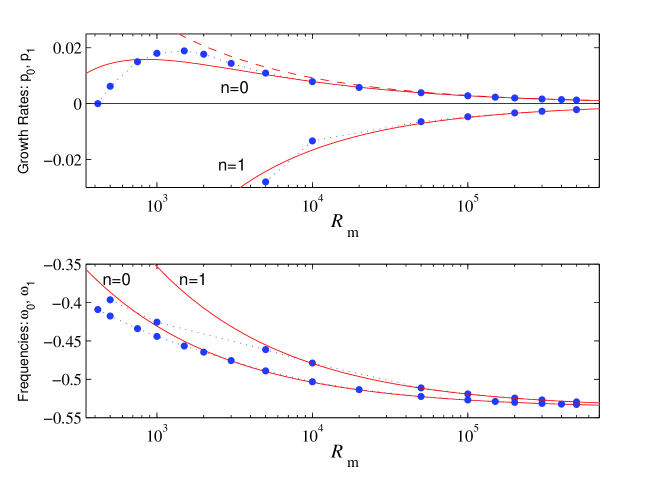
Figure 3: The growth rates and angular frequencies of the two leading modes of the $\mathbf{v}_{1}$ flow. These are characterised by $m=1$, $k=1$, and $n=0$ or $n=1$. The solid line represents the asymptotic expressions with the extra terms of Gilbert & Ponty (2000), the dashed line represents the asymptotic expression correct to order $\varepsilon^{2}$, the points on the dotted line represent the full numerical eigensolution.

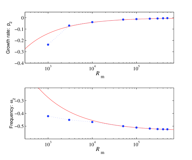
Figure 4: The growth rate $p_{2}$ and angular frequency $\omega_{2}$ for the $m=1$, $k=1$, $n=2$ mode of $\mathbf{v}_{1}$.

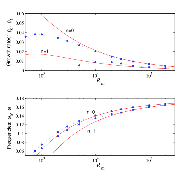
Figure 5: The growth rates and angular frequencies of the leading two modes of the $\mathbf{v}_{2}$ dynamo. Here $m=1$, $k=1$ and $n=0$ or $n=1$.

In Figs 3 and 4 we directly compare the predictions of the asymptotic theory and the numerical computations of the full eigenproblem for $\mathbf{v}_{1}$. Here is presented the numerical growth rate $\text{Re}\,\lambda$, and associated angular frequency $\text{Im}\,\lambda$, of the leading modes as a function of $R_{\text{m}}$. Alongside these data points, we plot the asymptotic growth rates $p_{i}$ and frequencies $\omega_{i}$, calculated with (a) the higher order terms of GP included (the solid lines), (b) the asymptotic theory correct to order $\varepsilon^{2}$ (the dashed line). The truncation levels for the asymptotic values are $K=400$. Note that both growth rates are scaled on the turnover time. This makes clear that the numerical growth rate goes to zero as $R_{\text{m}}\to\infty$. Helical dynamos are ‘slow’, as expected (Childress and Gilbert 1995, GP). Of the three modes shown, only the $n=0$ mode is a dynamo, which is active above a critical magnetic Reynolds number of $R_{\text{m}}\approx 416$ and achieves its maximum positive growth rate at $R_{\text{m}}\approx 1500$. In Fig. 5 we plot the growth rates and frequencies of the leading two modes of the $\mathbf{v}_{2}$ dynamo, for $m=k=1$. Both of these modes may grow for sufficiently large $R_{\text{m}}$.

Plainly, there is excellent agreement between the $n=0$ asymptotic growth rates and the numerical growth rates when $R_{\text{m}}\!\gtrsim\!10^{4}$ for both $\mathbf{v}_{1}$ and $\mathbf{v}_{2}$. The angular frequencies agree at smaller $R_{\text{m}}$. Fig.3 also shows that the additional terms of GP at higher order $\varepsilon^{4}$ improve the accuracy of the asymptotics markedly, in comparison with the theory up to $\varepsilon^{2}$ (the dashed line). This agreement strongly supports the asymptotic theory. It also indicates that the identification of the numerical modes with the asymptotic modes is correct. Finally, this shows that these flows only admit Ponomarenko-type dynamos in the large $R_{\text{m}}$ regime.

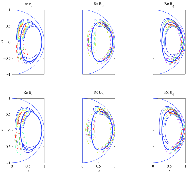
Figure 6: Plots of the magnetic eigenfunctions: the real parts of ${\hat{B}}_{r}$, ${\hat{B}}_{\theta}$, ${\hat{B}}_{\phi}$, for the $m=1$, $k=1$, $n=0$ mode upon the $\mathbf{v}_{1}$ flow. Here $\sigma=\sigma_{1}(1,1,\Psi_{0})$ and $R_{\text{m}}=10^{5}$. The three upper panels present the numerical eigensolution, while the lower three panels present the asymptotic eigensolution. Both numerical and asymptotic eigenfunctions have been normalised so that $|\hat{}\mathbf{B}|=1$, and each component has been plotted with 10 contours of equal increments.

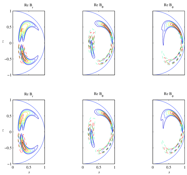
Figure 7: Plots of the real parts of the magnetic eigenfunctions: as in Figure 6 but with $R_{\text{m}}=5\times 10^{5}$.

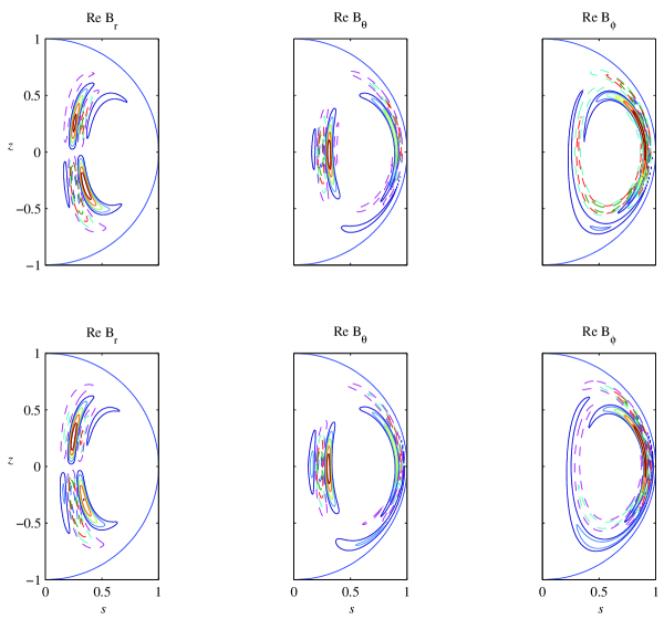
Figure 8: Plots of the magnetic eigenfunctions: the real part of the $n=1$ eigenmode, with $k=m=1$ and $R_{\text{m}}=5\times 10^{5}$ upon flow $\mathbf{v}_{1}$..

4.3 Magnetic field structure

Figures 6–8 show the real parts of the magnetic eigenfunctions for different values of $R_{\text{m}}$ and $n$ upon the $\mathbf{v}_{1}$ flow. These choices reveal the salient physical and asymptotic features of these modes. The morphologies of the $\mathbf{v}_{2}$ dynamos are much the same and are omitted in the interests of space.

In Fig. 6 we plot the magnetic field components, ${\hat{B}}_{r}$, ${\hat{B}}_{\theta}$, ${\hat{B}}_{\phi}$, of the $m=1$, $k=1$, $n=0$ mode. Here $\sigma=\sigma_{1}(1,1,\Psi_{0})$ and we set the magnetic Reynolds number to $R_{\text{m}}=10^{5}$. The top three panels present the numerical eigensolutions, while the bottom three panels show the asymptotic approximations. Superimposed upon the first set of figures is the resonant stream curve, which helps highlight the localisation of the magnetic field.

It is apparent from the figures that the asymptotic and numerical magnetic fields agree in their dominant features: the position, orientation and shape of the local maxima and minima. The localisation of the field to the resonant streamline is readily observed, with marked flux expulsion inside and outside the resonant streamline, as expected. In addition, the $k=1$ nature of the field is clear from its variation around the streamline, especially in $\hat{B}_{\phi}$. Note, however, that there is a slight offset outwards away from the resonant streamline in the upper numerical eigenfunctions. This offset in combination with the steep spatial gradients means the relative error between the asymptotic and numerical eigenfunctions is larger than expected. The relative error, defined by $\|\mathbf{B}^{\text{num}}-\mathbf{B}^{\text{asym}}\|_{2}/\|\mathbf{B}^{\text{num}}\|_{2}$, is 0.334 for this $R_{\text{m}}=10^{5}$ case.

In Fig. 7 we show the same mode but for larger magnetic Reynolds number: $R_{\text{m}}=5\times 10^{5}$. The resonant stream curve has been omitted. The magnetic field is more localised and intense, with the offset of the maxima and minima from the resonant streamline substantially reduced. Now the magnitudes of the numerical and asymptotic eigenfunction, in addition to the orientation of the magnetic features, are in good agreement. The relative error is reduced to 0.285.

The more involved $n=1$ eigenmode is plotted in Figure 8. The other parameters are kept the same and $R_{\text{m}}=5\times 10^{5}$. This mode decays slowly with time as shown in Figure 3. Its structure is more complicated due to the variation with $\psi$ under the gaussian envelope of $D_{1}(\Upsilon/\kappa)$. In particular, the field components vanish on the resonant streamline. The agreement between the asymptotic and numerical eigenfunctions is good but not as striking as in the $n=0$ case. In particular, the relative magnitudes of the maxima and minima are not in agreement, though the general shape of the structures are. This is possibly due to the fact that the mode has not fully converged to its asymptotic form. On the other hand, its greater spatial variation may be taxing the resolution of our numerical scheme, leading to errors.

5 Conclusions

In this paper we have compared the asymptotic theory of Gilbert & Ponty (2000) for axisymmetric roll dynamos in a sphere to the numerically computed results of the exact dynamo problem for two simple flows, with azimuthal components of the special form $v_{\phi}=r\sin\theta\,W(\psi)$ and of a more general form. In the regime $R_{\text{m}}\gtrsim 10^{4}$ excellent agreement is obtained between the asymptotic theory to $\mathcal{O}(R_{\text{m}}^{-1/2})$ and the numerical results for the growth rate and angular frequency. For the magnetic field the agreement between the asymptotic theory at leading order and the numerical results is good if $R_{\text{m}}=10^{5}$ and excellent if $R_{\text{m}}=5\!\times\!10^{5}$. The asymptotic formulas for the growth rate and the angular frequency have been extended in Appendix A in the Supplemental Material.

Only the simplest class of axisymmetric roll dynamos have been considered: those which consist of a single-roll flow with a single resonant streamline. The magnetic field in these dynamos is localised to the resonant stream surface and can interact only with itself. Further work is required on more complicated spherical roll flows: such as those those with a single-roll but more than one resonant streamline, and those with several rolls. These flows offer the possibility of interaction between magnetic fields localised to separate regions of the flow. This may produce interacting modes of non-Ponomarenko type, e.g. Gailitis type modes, alongside the Ponomarenko type modes (Gailitis 1970, 1993, 1995, Moss 2006). A related question, which arises from the localised nature of the Ponomarenko modes, is whether they depend on the magnetic boundary conditions at the surface of the conducting fluid.

Of key interest to both laboratory and astrophysical applications are (a) the nonlinear saturation of such modes and (b) their relationship to a background of small-scale velocity fluctuations. How will the dynamo modes back react on the helical flow which generated them? Will these modes build up magnetic torques which stifle the meridional motion, or will a more complicated dynamical interplay arise? If fluctuations are indeed present, for what size amplitudes, and for what correlation times and lengths, will they succesfully impede the satisfaction of the resonance condition which is so crucial for the formation of Ponomarenko modes? Recent work in cylindrical geometry for time-dependent fluctuations shows that Ponamarenko-type dynamo action can, in fact, survive in certain cases (Peyrot et al. 2007, 2008). But this need not be the case at all for flows exhibiting small-scale variations in space, and it is the latter situation which is probably most relevant in applications.

Spherical single-roll dynamos at large magnetic Reynolds number: Supplemental material

Appendix A Derivation of asymptotic expressions at large $R_{\text{m}}$

In this appendix we briefly derive the leading order results of the GP asymptotic theory presented in Section 3 of the main manuscript ‘Spherical single-roll dynamocs at large magnetic Reynolds number’. Once these are given we sketch out a technique whereby higher order terms may be calculated and give the solution to order $\varepsilon^{3}$. Note that reference labels for equations in the main manuscript are not preceded by either an ‘A’ or ‘B’.

A.1 Preliminaries

A.1.1 The magnetic diffusion term in toroidal coordinates

We take as our starting point the magnetic induction equation in the toroidal coordinate system $(\psi,\,\vartheta,\,\zeta)$, Eqs (3.19)-(3.21) in the main manuscript. In order to progress, the diffusion terms on the right sides need to be decomposed into their component parts.

Using the summation convention the magnetic field can be written as $\mathbf{B}=B^{i}\mathbf{f}_{i}$, the gradient operator as $\nabla=(\nabla\psi^{i})\partial_{i}$, where $\partial_{i}=\partial_{\psi^{i}}$, and the diffusion term in the magnetic induction equation as $\nabla^{2}\mathbf{B}=(\nabla^{2}B^{j})\mathbf{f}_{j}+2\nabla B^{j}\cdot\nabla\mathbf{f}_{j}+B^{j}\nabla^{2}\mathbf{f}_{j}$. Thus, since $\nabla B^{j}=(\partial_{k}B^{j})\nabla\psi^{k}$, the covariant components of this term are

$$\nabla\psi^{i}\cdot\nabla^{2}\mathbf{B}=(\nabla^{2}B^{i})+2(\partial_{k}B^{j})\nabla\psi^{k}\cdot\nabla\mathbf{f}_{j}\cdot\nabla\psi^{i}+B^{j}\nabla\psi^{i}\cdot\nabla^{2}\mathbf{f}_{j}\,.$$

Four of the 27 terms $\nabla\psi^{k}\cdot\nabla\mathbf{f}_{j}\cdot\nabla\psi^{i}$ and three of the 9 terms $\nabla\psi^{i}\cdot\nabla^{2}\mathbf{f}_{j}$ vanish identically, since $\nabla\mathbf{f}_{\zeta}=\mathbf{1}_{s}\mathbf{1}_{\phi}-\mathbf{1}_{\phi}\mathbf{1}_{s}$ means that $\mathbf{a}\cdot(\nabla\mathbf{f}_{\zeta})\cdot\mathbf{b}=0$ for any meridional vectors $\mathbf{a}$, $\mathbf{b}$. We then have

$$\nabla\psi\cdot(\nabla\psi\cdot\nabla\mathbf{f}_{\zeta})=\nabla\psi\cdot(\nabla\vartheta\cdot\nabla\mathbf{f}_{\zeta})=\nabla\vartheta\cdot(\nabla\psi\cdot\nabla\mathbf{f}_{\zeta})=\nabla\vartheta\cdot(\nabla\vartheta\cdot\nabla\mathbf{f}_{\zeta})=0\,.$$

Also $\nabla^{2}\mathbf{f}_{\zeta}=\mathbf{0}$ implies $\nabla\psi\cdot\nabla^{2}\mathbf{f}_{\zeta}=\nabla\vartheta\cdot\nabla^{2}\mathbf{f}_{\zeta}=\nabla\zeta\cdot\nabla^{2}\mathbf{f}_{\zeta}=0$.

Keeping only terms which appear later in the asymptotic analysis and suppressing the others with dots, the relevant diffusion terms are

$$\nabla\psi\cdot\nabla^{2}\mathbf{B} =(\nabla^{2}+2\mu_{i}\partial_{\psi}+2\mu_{j}\partial_{\vartheta}+2\mu_{k}\partial_{\zeta}+\mu_{l})B_{\psi}$$

$$\hskip 85.35826pt+(2\mu_{a}\partial_{\psi}+2\mu_{b}\partial_{\vartheta}+2\mu_{c}\partial_{\zeta}+\mu_{d})B_{\vartheta}+2\mu_{g}\partial_{\zeta}B_{\zeta}$$ (A.34)

$$\nabla\vartheta\cdot\nabla^{2}\mathbf{B} =(\nabla^{2}+2\lambda_{a}\partial_{\psi}+2\lambda_{b}\partial_{\vartheta}+2\lambda_{c}\partial_{\zeta}+\lambda_{d})B_{\vartheta}+2\lambda_{g}\partial_{\zeta}B_{\zeta}+\dots$$ (A.35)

$$\nabla\zeta\cdot\nabla^{2}\mathbf{B} =2\rho_{a}\partial_{\psi}B_{\vartheta}+(\nabla^{2}+2\rho_{b}\partial_{\psi})B_{\zeta}+\dots\,,$$ (A.36)

where the coefficients are defined by

$$\mu_{a} =\nabla\psi\cdot(\nabla\psi\cdot\nabla\mathbf{f}_{\vartheta}) \mu_{b} =\nabla\psi\cdot(\nabla\vartheta\cdot\nabla\mathbf{f}_{\vartheta}) \mu_{c} =\nabla\psi\cdot(\nabla\zeta\cdot\nabla\mathbf{f}_{\vartheta}) \mu_{d} =\nabla\psi\cdot\nabla^{2}\mathbf{f}_{\vartheta}$$

$$\mu_{g} =\nabla\psi\cdot(\nabla\zeta\cdot\nabla\mathbf{f}_{\zeta}) \mu_{i} =\nabla\psi\cdot(\nabla\psi\cdot\nabla\mathbf{f}_{\psi}) \mu_{j} =\nabla\psi\cdot(\nabla\vartheta\cdot\nabla\mathbf{f}_{\psi}) \mu_{k} =\nabla\psi\cdot(\nabla\zeta\cdot\nabla\mathbf{f}_{\psi})$$

$$\mu_{l} =\nabla\psi\cdot\nabla^{2}\mathbf{f}_{\psi} \lambda_{a} =\nabla\vartheta\cdot(\nabla\psi\cdot\nabla\mathbf{f}_{\vartheta}) \lambda_{b} =\nabla\vartheta\cdot(\nabla\vartheta\cdot\nabla\mathbf{f}_{\vartheta}) \lambda_{c} =\nabla\vartheta\cdot(\nabla\zeta\cdot\nabla\mathbf{f}_{\vartheta})$$

$$\lambda_{d} =\nabla\vartheta\cdot\nabla^{2}\mathbf{f}_{\vartheta} \lambda_{g} =\nabla\vartheta\cdot(\nabla\zeta\cdot\nabla\mathbf{f}_{\zeta}) \rho_{a} =\nabla\zeta\cdot(\nabla\psi\cdot\nabla\mathbf{f}_{\vartheta}) \rho_{b} =\nabla\zeta\cdot(\nabla\psi\cdot\nabla\mathbf{f}_{\zeta})\,.$$

Apart from $\mu_{d}$, $\mu_{l}$, $\lambda_{d}$ these are Christoffel symbols.

The scalar Laplacian is $\nabla^{2}=\nabla\cdot(\nabla\psi^{i})\partial_{i}=(\nabla\psi^{i}\cdot\nabla\psi^{j})\partial_{i}\partial_{j}+(\nabla^{2}\psi^{i})\partial_{i}$, which, in full, can be expressed as

$$\nabla^{2}=(\nabla\psi)^{2}\partial^{2}_{\psi}+2(\nabla\psi\cdot\nabla\vartheta)\partial_{\psi}\partial_{\vartheta}+(\nabla\vartheta)^{2}\partial^{2}_{\vartheta}+2(\nabla\vartheta\cdot\nabla\zeta)\partial_{\vartheta}\partial_{\zeta}\\ +(\nabla\zeta)^{2}\partial^{2}_{\zeta}+2(\nabla\zeta\cdot\nabla\psi)\partial_{\zeta}\partial_{\psi}+(\nabla^{2}\psi)\partial_{\psi}+(\nabla^{2}\vartheta)\partial_{\vartheta}+(\nabla^{2}\zeta)\partial_{\zeta}\,.$$

Furthermore, a number of the geometric coefficients average to zero,

$$\overline{\mu}_{a}=\overline{\mu}_{d}=\overline{\mu}_{g}=\overline{\mu}_{l}=\overline{\lambda}_{b}=\overline{\rho}_{b}=0\,,$$ (A.37)

which can be established using standard vector identities, the divergence theorem and Stokes’ theorem (see GP).

A.1.2 Explicit asymptotic expansions

We now employ the asymptotic scalings presented in Section 3.2 and the order one variable $\varUpsilon$, and then choose a specific streamsurface $\psi=\psi_{0}$ around which we expand.

The $\psi$-derivatives and gradient operators in Eqs (3.19)-(3.21) become

$$\partial_{\psi}=\varepsilon^{-1}\partial_{\varUpsilon}\,,\qquad\nabla=\varepsilon^{-1}\nabla\psi\,\partial_{\varUpsilon}+\nabla\vartheta\,\partial_{\vartheta}+\nabla\zeta\,\partial_{\zeta}\,,$$ (A.38)

and the magnetic field components take the functional forms,

$$B_{\psi}=\varepsilon^{2}b_{\psi}(\varUpsilon,\vartheta)e^{im\zeta+i\omega t+pt}\,,\quad B_{\vartheta}=b_{\vartheta}(\varUpsilon,\vartheta)e^{im\zeta+i\omega t+pt}\,,\quad B_{\zeta}=b_{\zeta}(\varUpsilon,\vartheta)e^{im\zeta+i\omega t+pt}\,.$$ (A.39)

We now expand $\omega$ and $p$ in powers of $\varepsilon$ with the ordering (3.22),

$$\omega=\omega_{0}+\varepsilon\omega_{1}+\varepsilon^{2}\omega_{2}+\varepsilon^{3}\omega_{3}+\varepsilon^{4}\omega_{5}+\dots\,,\quad p=\varepsilon^{2}p_{2}+\varepsilon^{3}p_{3}+\varepsilon^{4}p_{4}+\dots\,,$$ (A.40)

and expand $\overline{W}(\psi)$ and $\Omega(\psi)$ in Taylor series about the streamline $\psi=\psi_{o}$,

$$\Omega(\psi_{o}+\varepsilon\varUpsilon) =\Omega_{o}+\Omega^{\prime}_{o}\varepsilon\varUpsilon+\tfrac{1}{2}\Omega^{\prime\prime}_{o}\varepsilon^{2}\varUpsilon^{2}+\dots$$ (A.41)

$$\overline{W}(\psi_{o}+\varepsilon\varUpsilon) =\overline{W}_{o}+\overline{W}^{\prime}_{o}\varepsilon\varUpsilon+\tfrac{1}{2}\overline{W}^{\prime\prime}_{o}\varepsilon^{2}\varUpsilon^{2}+\dots\,,$$ (A.42)

in which $\Omega_{o}=\Omega(\psi_{o})$, $\Omega^{\prime}_{o}=\Omega^{\prime}(\psi_{o})$, etc. Assuming the functional dependencies of (A.39) and substituting the expansions (A.40)–(A.42) into the advection operator (3.17) gives

$$D_{t}=d_{0}+\varepsilon d_{1}+\varepsilon^{2}d_{2}+\varepsilon^{3}d_{3}+\varepsilon^{4}d_{4}+\dots\,,$$ (A.43)

where

$$d_{n}=p_{n}+i\omega_{n}+\frac{\varUpsilon^{n}}{n!}\Big{(}\Omega^{(n)}_{o}\partial_{\vartheta}+im\overline{W}^{(n)}_{o}\Big{)}\,,\quad p_{0}=p_{1}=0\,.$$ (A.44)

We also expand $(\nabla\psi)^{2}$ in the diffusion term,

$$(\nabla\psi)^{2}=\gamma_{0}+\varepsilon\varUpsilon\gamma_{1}+\varepsilon^{2}\varUpsilon^{2}\gamma_{2}+\varepsilon^{3}\varUpsilon^{3}\gamma_{3}+\varepsilon^{4}\varUpsilon^{4}\gamma_{4}+\dots\,$$ (A.45)

as well as the individual ‘diffusion coefficients’, for example:

$$\mu_{b}=\mu_{b,0}+\varepsilon\varUpsilon\mu_{b,1}+\dots.$$

Finally we expand the magnetic field components,

$$b_{\psi}=b_{\psi 0}+\varepsilon b_{\psi 1}+\dots\,,\quad b_{\vartheta}=b_{\vartheta 0}+\varepsilon b_{\vartheta 1}+\dots\,,\quad b_{\zeta}=b_{\zeta 0}+\varepsilon b_{\zeta 1}+\dots\,.$$ (A.46)

We are now ready to derive the asymptotic equations at the various orders.

A.2 The $\varepsilon^{0}$ equations

In this and the following two subsections we describe the asymptotics to order $\varepsilon^{2}$. We substitute expansions (A.40)–(A.43), (A.45) and (A.46) into the component equations (3.19)–(3.21), divide (3.19) by $\varepsilon^{2}$, and collect terms of like order.

The $\varepsilon^{0}$-equations are

$$d_{0}b_{\psi 0}=0\,,\qquad d_{0}b_{\vartheta 0}=0\,,\qquad d_{0}b_{\zeta 0}=0\,,$$ (A.47)

which have the solution,

$$b_{\psi 0}=F_{\psi 0}(\varUpsilon)e^{ik\vartheta}\,,\quad b_{\vartheta 0}=F_{\vartheta 0}(\varUpsilon)e^{ik\vartheta}\,,\quad b_{\zeta 0}=F_{\zeta 0}(\varUpsilon)e^{ik\vartheta}\,,$$ (A.48)

where the functions $F_{\psi 0}$, $F_{\vartheta 0}$, $F_{\zeta 0}$ are determined at order $\varepsilon^{2}$ and must vanish as $|\varUpsilon|\to\infty$. The constant $k$ is an integer since $\mathbf{B}$ is single-valued. Solvability of (A.47) fixes the angular frequency $\omega$ to leading order for given $m$ and $k$,

$$\omega_{0}=-\Pi_{o}\,,$$ (A.49)

where we have introduced the advection frequency function $\Pi(\psi)=k\Omega+m\overline{W}$. The operator $d_{0}$ becomes $\Omega_{o}(\partial_{\vartheta}-ik)$, and hence annihilates any term with the $\vartheta$-dependence $e^{ik\vartheta}$.

A.3 The $\varepsilon^{1}$ equations

The $\varepsilon^{1}$-equations are

$$d_{0}b_{\psi 1}+d_{1}b_{\psi 0}=2\mu_{a,o}\partial_{\varUpsilon}b_{\vartheta 0}\,,\quad d_{0}b_{\vartheta 1}+d_{1}b_{\vartheta 0}=0\,,\quad d_{0}b_{\zeta 1}+d_{1}b_{\zeta 0}=0\,.$$ (A.50)

Their solvability requires

$$\omega_{1}=0\,,\qquad\Pi^{\prime}_{o}=k\Omega^{\prime}_{o}+m\overline{W}^{\prime}_{o}=0\,.$$ (A.51)

The last condition fixes the resonant streamline $\psi=\psi_{o}$, upon which the magnetic field is localised for given $m$ and $k$. At this streamline the function $\Pi(\psi)$ possesses a critical point, and a maximum if $\Pi^{\prime\prime}_{o}<0$, which is the case for the simple roll flows we examine. The larger gradients in $B_{\vartheta}$ and $B_{\zeta}$ on this surface encourage diffusion of these fields and hence replenishment of $B_{\psi}$. The operator $d_{1}$ becomes $d_{1}=\Upsilon\Omega^{\prime}_{o}(\partial_{\vartheta}-ik)$ and hence also annihilates any term with $\vartheta$-dependence $e^{ik\vartheta}$.

The last two equations in (A.50) can be solved similarly to (A.47). The first equation reduces to,

$$d_{0}b_{\psi 1}=2\mu_{a,o}\partial_{\varUpsilon}b_{\vartheta 0}=2\mu_{a,o}F^{\prime}_{\vartheta 0}(\varUpsilon)e^{ik\vartheta}\,,$$

which is solvable, since $\overline{\mu}_{a}=0$ and the right side then possesses no term with the $\vartheta$-dependence $e^{ik\vartheta}$. Thus the magnetic field at order $\varepsilon^{1}$ is

$$b_{\psi 1}=F_{\psi 1}(\varUpsilon)e^{ik\vartheta}+G_{\psi 1}(\varUpsilon,\vartheta)e^{ik\vartheta}\,,\quad b_{\vartheta 1}=F_{\vartheta 1}(\varUpsilon)e^{ik\vartheta}\,,\quad b_{\zeta 1}=F_{\zeta 1}(\varUpsilon)e^{ik\vartheta}\,,$$ (A.52)

where the functions $F_{\psi 1}$, $F_{\vartheta 1}$, $F_{\zeta 1}$ are determined at order $\varepsilon^{3}$ and the particular integral for equation (A.50)(a) is

$$G_{\psi 1}=\frac{2F^{\prime}_{\vartheta 0}}{\Omega_{o}}\widehat{\mu}_{a,o}\,,\qquad\overline{G_{\psi 1}}=0\,.$$ (A.53)

Here we have introduced the hat operator $\ \widehat{}\$ defined by

$$\partial_{\vartheta}\widehat{f}\equiv f-\overline{f}\,,\qquad\overline{\!\widehat{f}\>}=0\,,$$

which implies

$$\widehat{f}=\int_{0}^{\vartheta}(f-\overline{f})\,d\vartheta-\overline{\int_{0}^{\vartheta}(f-\overline{f})\,d\vartheta}\,.$$

In addition, the properties

$$\overline{\widehat{f}g}=-\overline{f\widehat{g}\>}\,,\qquad\overline{f\widehat{f}\>}=0$$ (A.54)

are easily established.

A.4 The $\varepsilon^{2}$ equations

The $\varepsilon^{2}$-equations are

$$d_{0}b_{\psi 2}+d_{1}b_{\psi 1}+(d_{2}-\gamma_{0}\partial^{2}_{\varUpsilon})b_{\psi 0} =2\mu_{a,o}\partial_{\varUpsilon}b_{\vartheta 1}+2\mu^{\prime}_{a,o}\varUpsilon\partial_{\varUpsilon}b_{\vartheta 0}$$

$$+(2\mu_{b,o}\partial_{\vartheta}+2im\mu_{c,o}+\mu_{d,o})b_{\vartheta 0}+2im\mu_{g,o}b_{\zeta 0}$$ (A.55)

$$d_{0}b_{\vartheta 2}+d_{1}b_{\vartheta 1}+(d_{2}-\gamma_{0}\partial^{2}_{\varUpsilon})b_{\vartheta 0} =\Omega^{\prime}_{o}b_{\psi 0}$$ (A.56)

$$d_{0}b_{\zeta 2}+d_{1}b_{\zeta 1}+(d_{2}-\gamma_{0}\partial^{2}_{\varUpsilon})b_{\zeta 0} =\overline{W}^{\prime}_{o}b_{\psi 0}\,.$$ (A.57)

GP included subdominant terms from the Laplacian at this order arguing that these are comparable when employing the scalings of Gilbert (1988). However, they neglect to include the coordinate Laplacians, $\nabla^{2}\psi$, $\nabla^{2}\vartheta$, $\nabla^{2}\zeta$ which should be of the same order. In the present analysis all these terms appear at the correct (higher) orders.

Equations (A.55)–(A.57) are solvable for the field components $b_{\psi 2}$, $b_{\vartheta 2}$ and $b_{\zeta 2}$, if the $\vartheta$-dependence of the other terms is not $e^{ik\vartheta}$. This is true for the terms, $d_{1}b_{\psi 1}$, $d_{1}b_{\vartheta 1}$ and $d_{1}b_{\zeta 1}$, since the operator $d_{1}$ annihilates $e^{ik\vartheta}$. It is also satisfied by the terms, $2\mu_{a,o}\partial_{\varUpsilon}b_{\vartheta 1}$, $2\mu_{d,o}b_{\vartheta 0}$ and $2im\mu_{g,o}b_{\zeta 0}$, since the coefficients $\mu_{a,o}$, $\mu_{d,o}$, $\mu_{g,o}$ average to zero by (A.37). The sum of the remaining terms must average to zero after multiplication by $e^{-ik\vartheta}$. Consequently we may write the solvability condition for (A.55)–(A.57) as

$$\mathbf{L}\left(\begin{matrix}F_{\psi 0}\\ F_{\vartheta 0}\\ F_{\zeta 0}\end{matrix}\right)=\mathbf{0}\,,\qquad\mathbf{L}=\left(\begin{matrix}\Xi&2i\overline{\alpha}_{o}&0\\ \Omega^{\prime}_{o}&\Xi&0\\ \overline{W}^{\prime}_{o}&0&\Xi\end{matrix}\right)\,,$$ (A.58)

where

$$\Xi=\overline{\gamma}_{0}\partial_{\varUpsilon}^{2}-\tfrac{1}{2}i\Pi^{\prime\prime}_{o}\varUpsilon^{2}-p_{2}-i\omega_{2}\,,\qquad\alpha=k\mu_{b}+m\mu_{c}\,,\qquad\Pi^{\prime\prime}_{o}=k\Omega^{\prime\prime}_{o}+m\overline{W}^{\prime\prime}_{o}\,,$$ (A.59)

with $\overline{\gamma}_{0}=<|\nabla\psi|_{o}^{2}>$. These equations determine the functions $F_{\psi 0}$, $F_{\vartheta 0}$, $F_{\zeta 0}$ and hence the magnetic field to leading order. The solutions are of the form

$$\left(\begin{matrix}F_{\psi 0}\\ F_{\vartheta 0}\\ F_{\zeta 0}\end{matrix}\right)=y_{n}(\varUpsilon)\mathbf{a}\,,\qquad y_{n}(\varUpsilon)=\operatorname{D}_{n}\left(\varUpsilon/\kappa\right),\qquad\kappa=(\overline{\gamma}_{0}/2i\Pi^{\prime\prime}_{o})^{1/4}.$$ (A.60)

Here $\mathbf{a}$ is a constant vector to be determined and $\operatorname{D}_{n}(z)$ is the parabolic cylinder function of degree $n$,

$$\operatorname{D}_{n}(z)=2^{-n/2}e^{-z^{2}/4}\operatorname{H}_{n}(z/\sqrt{2})\,,\qquad n\geq 0\,,$$

where $\operatorname{H}_{n}(z)$ is the Hermite polynomial of degree $n$ (Abramowitz & Stegun 1972). In order for this solution to satisfy the boundary conditions, i.e. $F_{\psi 0},F_{\vartheta 0},F_{\zeta 0}\to 0$ as $|\varUpsilon|\to\infty$, we choose $\kappa^{-2}$ with positive real part,

$$\kappa^{-2}=\sqrt{|\Pi^{\prime\prime}_{o}|/\overline{\gamma}_{0}}\ (1+i\operatorname{sgn}\Pi^{\prime\prime}_{o})\,,$$

noting that $\overline{\gamma}_{0}>0$. The two eigenfunctions which arise from the ambiguous sign of $\kappa$ differ only if $n$ is odd and then only in sign. Thus

$$\kappa^{-1}=\sqrt[4]{2|\Pi^{\prime\prime}_{o}|/\overline{\gamma}_{0}}\ e^{i\pi(\operatorname{sgn}\Pi^{\prime\prime}_{o})/8}=\sqrt[4]{|\Pi^{\prime\prime}_{o}|/\overline{\gamma}_{0}}\bigg{(}\sqrt{\tfrac{\sqrt{2}+1}{2}}+i\sqrt{\tfrac{\sqrt{2}-1}{2}}\ \operatorname{sgn}\Pi^{\prime\prime}_{o}\bigg{)}\,.$$

The $y_{n}$ are eigenfunctions of $\Xi$ with eigenvalue $\xi_{n}$,

$$\Xi y_{n}=\xi_{n}y_{n}\,,\qquad\xi_{n}=-(n+\tfrac{1}{2})\sqrt{|\Pi^{\prime\prime}_{o}|\overline{\gamma}_{0}}\ (1+i\operatorname{sgn}\Pi^{\prime\prime}_{o})-(p_{2}+i\omega_{2})\,.$$

Substitution of the ansatz (A.60) into (A.58) gives

$$\mathbf{L}_{n}\mathbf{a}=\mathbf{0}\,,\qquad\mathbf{L}_{n}=\left(\begin{matrix}\xi_{n}&2i\overline{\alpha}_{o}&0\\ \Omega^{\prime}_{o}&\xi_{n}&0\\ \overline{W}^{\prime}_{o}&0&\xi_{n}\end{matrix}\right)\,,$$ (A.61)

which has non-trivial solutions if $\det\mathbf{L}_{n}=0$. This yields $\xi_{n}=0$ or $\xi_{n}^{2}=2i\overline{\alpha}_{o}\Omega^{\prime}_{o}$, i.e. $\xi_{n}=\pm(1+i\operatorname{sgn}\overline{\alpha}_{o}\Omega^{\prime}_{o})\sqrt{|\overline{\alpha}_{o}\Omega^{\prime}_{o}|}$, and determines $p_{2}$ and $\omega_{2}$. We shall ignore the solution for $\xi_{n}=0$, since its growth rate has a negative real part. The other two solutions give for the $n$th mode

$$p_{2} =\mp\sqrt{|\overline{\alpha}_{o}\Omega^{\prime}_{o}|}-(n+\tfrac{1}{2})\sqrt{|\Pi^{\prime\prime}_{o}|\overline{\gamma}_{0}}$$ (A.62)

$$\omega_{2} =\mp\sqrt{|\overline{\alpha}_{o}\Omega^{\prime}_{o}|}\ \operatorname{sgn}(\overline{\alpha}_{o}\Omega^{\prime}_{o})-(n+\tfrac{1}{2})\sqrt{|\Pi^{\prime\prime}_{o}|\overline{\gamma}_{0}}\,\operatorname{sgn}\Pi^{\prime\prime}_{o}$$ (A.63)

$$\mathbf{a} =[-\xi_{n},\Omega^{\prime}_{o},\overline{W}^{\prime}_{o}]^{T}\,.$$ (A.64)

The real and imaginary parts of the growth rate in (A.62) and (A.63) agree with Gilbert & Ponty (2000) to order $\epsilon^{2}$. The vector $\mathbf{a}$ is determined up to a constant factor.

Equations (A.55)–(A.57) have solutions of the form,

$$b_{\psi 2} =F_{\psi 2}(\varUpsilon)e^{ik\vartheta}+G_{\psi 2}(\varUpsilon,\vartheta)e^{ik\vartheta}\,,\qquad\overline{G}_{\psi 2}=0$$ (A.65)

$$b_{\vartheta 2} =F_{\vartheta 2}(\varUpsilon)e^{ik\vartheta}+G_{\vartheta 2}(\varUpsilon,\vartheta)e^{ik\vartheta}\,,\qquad\overline{G}_{\vartheta 2}=0$$ (A.66)

$$b_{\zeta 2} =F_{\zeta 2}(\varUpsilon)e^{ik\vartheta}+G_{\zeta 2}(\varUpsilon,\vartheta)e^{ik\vartheta}\,,\qquad\overline{G}_{\zeta 2}=0\,.$$ (A.67)

The particular integrals $G_{\psi 2}$, $G_{\vartheta 2}$ and $G_{\zeta 2}$ can be determined at this order by subtracting from (A.55)–(A.57) their projections on $e^{ik\vartheta}$ and integrating with respect to $\vartheta$. The results are

$$\Omega_{o}G_{\psi 2}=-\frac{2\Omega^{\prime}_{o}}{\Omega_{o}}\widehat{\mu}_{a,o}\varUpsilon F^{\prime}_{\vartheta 0}+\widehat{\gamma}_{0}F^{\prime\prime}_{\psi 0}+2\widehat{\mu}_{a,o}F^{\prime}_{\vartheta 1}+2\widehat{\mu}^{\prime}_{a,o}\varUpsilon F^{\prime}_{\vartheta 0}+(2i\widehat{\alpha}_{o}+\widehat{\mu}_{d,o})F_{\vartheta 0}+2im\widehat{\mu}_{g,o}F_{\zeta 0}\,.$$ (A.68)

$$\Omega_{o}G_{\vartheta 2}=\widehat{\gamma}_{0}F^{\prime\prime}_{\vartheta 0}\,.$$ (A.69)

$$\Omega_{o}G_{\zeta 2}=\widehat{\gamma}_{0}F^{\prime\prime}_{\zeta 0}\,.$$ (A.70)

A.5 The asymptotic theory to $\mathcal{O}(\varepsilon^{3})$ and beyond

In this subsection we compute the solution of the $\varepsilon^{3}$ equations and thus determine the magnetic field structure to $\varepsilon^{1}$ and that $p_{3}=\omega_{3}=0$. In so doing we sketch out a general method to compute the solution at higher orders.

The $\varepsilon^{3}$-equations are

$$d_{0}b_{\psi 3}+d_{1}b_{\psi 2}+(d_{2}-\gamma_{0}\partial_{\varUpsilon}^{2})b_{\psi 1}+(d_{3}-\gamma_{1}\varUpsilon\partial_{\varUpsilon}^{2})b_{\psi 0}=2(\chi_{0,1}+\mu_{i,o})\partial_{\varUpsilon}b_{\psi 0}\\ +2\mu_{a,o}\partial_{\varUpsilon}b_{\vartheta 2}+2\mu^{\prime}_{a,o}\varUpsilon\partial_{\varUpsilon}b_{\vartheta 1}+\mu^{\prime\prime}_{a,o}\varUpsilon^{2}\partial_{\varUpsilon}b_{\vartheta 0}+(2\mu_{b,o}\partial_{\vartheta}+2im\mu_{c,o}+\mu_{d,o})b_{\vartheta 1}\\ +(2\mu^{\prime}_{b,o}\partial_{\vartheta}+2im\mu^{\prime}_{c,o}+\mu^{\prime}_{d,o})\varUpsilon b_{\vartheta 0}+2im\mu_{g,o}b_{\zeta 1}+2im\mu^{\prime}_{g,o}\varUpsilon b_{\zeta 0}$$ (A.71)

$$d_{0}b_{\vartheta 3}+d_{1}b_{\vartheta 2}+(d_{2}-\gamma_{0}\partial_{\varUpsilon}^{2})b_{\vartheta 1}+(d_{3}-\gamma_{1}\varUpsilon\partial_{\varUpsilon}^{2})b_{\vartheta 0}=2(\chi_{1,o}+\lambda_{a,o})\partial_{\varUpsilon}b_{\vartheta 0}+\Omega^{\prime}_{o}b_{\psi 1}+\varUpsilon\Omega^{\prime\prime}_{o}b_{\psi 0}$$ (A.72)

$$d_{0}b_{\zeta 3}+d_{1}b_{\zeta 2}+(d_{2}-\gamma_{0}\partial_{\varUpsilon}^{2})b_{\zeta 1}+(d_{3}-\gamma_{1}\varUpsilon\partial_{\varUpsilon}^{2})b_{\zeta 0}=2(\chi_{1,o}+\rho_{b,o})\partial_{\varUpsilon}b_{\zeta 0}\\ +2\rho_{a,o}\partial_{\varUpsilon}b_{\vartheta 0}+\overline{W}^{\prime}_{o}b_{\psi 1}+\varUpsilon\overline{W}_{o}^{\prime\prime}b_{\psi 0}\,,$$ (A.73)

where we have introduced

$$\chi_{1}=\tfrac{1}{2}\nabla^{2}\psi+i(k\nabla\psi\cdot\nabla\vartheta+m\nabla\psi\cdot\nabla\zeta)\,.$$

Note that we can write $d_{2}-\gamma_{0}\partial_{\varUpsilon}^{2}=-\Xi+\tfrac{1}{2}\varUpsilon^{2}\Omega^{\prime\prime}_{o}(\partial_{\vartheta}-ik)-(\gamma_{0}-\overline{\gamma}_{0})\partial_{\varUpsilon}^{2}$.

The solutions of equations (A.71)–(A.73) can be written in the form,

$$b_{\psi 3} =F_{\psi 3}(\varUpsilon)e^{ik\vartheta}+G_{\psi 3}(\varUpsilon,\vartheta)e^{ik\vartheta}\,,\qquad\overline{G}_{\psi 3}=0$$ (A.74)

$$b_{\vartheta 3} =F_{\vartheta 3}(\varUpsilon)e^{ik\vartheta}+G_{\vartheta 3}(\varUpsilon,\vartheta)e^{ik\vartheta}\,,\qquad\overline{G}_{\vartheta 3}=0$$ (A.75)

$$b_{\zeta 3} =F_{\zeta 3}(\varUpsilon)e^{ik\vartheta}+G_{\zeta 3}(\varUpsilon,\vartheta)e^{ik\vartheta}\,,\qquad\overline{G}_{\zeta 3}=0\,.$$ (A.76)

Projecting equations (A.71)–(A.73) onto $e^{ik\vartheta}$ and using (A.37) gives

$$\Xi F_{\psi 1}+2i\overline{\alpha}_{o}F_{\vartheta 1} =(p_{3}+i\omega_{3}+\tfrac{1}{6}i\Pi^{\prime\prime\prime}_{o}\varUpsilon^{3}-\overline{\gamma}_{1}\varUpsilon\partial_{\varUpsilon}^{2})F_{\psi 0}-2(\overline{\chi}_{1,o}+\overline{\mu}_{i,o})F^{\prime}_{\psi 0}-2i\overline{\alpha}^{\prime}_{o}\varUpsilon F_{\vartheta 0}$$

$$\Xi F_{\vartheta 1}+\Omega^{\prime}_{o}F_{\psi 1} =(p_{3}+i\omega_{3}+\tfrac{1}{6}i\Pi^{\prime\prime\prime}_{o}\varUpsilon^{3}-\overline{\gamma}_{1}\varUpsilon\partial_{\varUpsilon}^{2})F_{\vartheta 0}-2(\overline{\chi}_{1,o}+\overline{\lambda}_{a,o})F^{\prime}_{\vartheta 0}-\varUpsilon\Omega^{\prime\prime}_{o}F_{\psi 0}$$

$$\Xi F_{\zeta 1}+\overline{W}^{\prime}_{o}F_{\psi 1} =(p_{3}+i\omega_{3}+\tfrac{1}{6}i\Pi^{\prime\prime\prime}_{o}\varUpsilon^{3}-\overline{\gamma}_{1}\varUpsilon\partial_{\varUpsilon}^{2})F_{\zeta 0}-2\overline{\chi}_{1,o}F^{\prime}_{\zeta 0}-2\overline{\rho}_{a,o}F^{\prime}_{\vartheta 0}-\varUpsilon\overline{W}_{o}^{\prime\prime}F_{\psi 0}\,,$$

since $\overline{G^{\prime}_{\psi 1}}=0$, $\overline{G^{\prime\prime}_{\psi 1}}=0$, $\overline{\mu}_{a,o}=\overline{\mu}^{\prime}_{a,o}=\overline{\mu}^{\prime\prime}_{a,o}=0$, $\overline{\mu}_{d,o}=\overline{\mu}^{\prime}_{d,o}=0$, $\overline{\mu}_{g,o}=\overline{\mu}^{\prime}_{g,o}=0$, $\overline{\rho}_{b,o}=0$. The primes on the $G$ functions denote differentiation with respect to $\varUpsilon$. Note from (A.53) and (A.69),

$$\overline{\gamma_{0}G^{\prime\prime}_{\psi 1}}+2\overline{\mu_{a,o}G^{\prime}_{\vartheta 2}}=\frac{2F^{\prime\prime\prime}_{\vartheta 0}}{\Omega_{o}}(\overline{\gamma_{0}\widehat{\mu}_{a,o}+\widehat{\gamma}_{0}\mu_{a,o}})=0\,.$$

In vector form the projected equations are

$$\mathbf{L}\mathbf{F}_{1}=\{(p_{3}+i\omega_{3})y_{n}+\tfrac{1}{6}i\Pi^{\prime\prime\prime}_{o}\varUpsilon^{3}y_{n}-\overline{\gamma}_{1}\varUpsilon y^{\prime\prime}_{n}-2\overline{\chi}_{1,o}y^{\prime}_{n}\}\mathbf{a}-\varUpsilon y_{n}\mathbf{a}_{1}-2y^{\prime}_{n}\mathbf{a}_{2}\,,$$ (A.77)

where $\mathbf{L}$ is defined in (A.58), $\mathbf{F}_{1}=(F_{\psi 1},F_{\vartheta 1},F_{\zeta 1})^{T}$ and

$$\mathbf{a}_{1}=[2i\overline{\alpha}^{\prime}_{o}\Omega^{\prime}_{o},-\Omega^{\prime\prime}_{o}\xi_{n},-\overline{W}^{\prime\prime}_{o}\xi_{n}]^{T}\,,\quad\mathbf{a}_{2}=[-\overline{\mu}_{i,o}\xi_{n},\overline{\lambda}_{a,o}\Omega^{\prime}_{o},\overline{\rho}_{a,o}\Omega^{\prime}_{o}]^{T}\,.$$ (A.78)

The primes on $y_{n}$ indicate derivatives with respect to $\varUpsilon$.

We next express the derivatives and terms multiplied by $\varUpsilon$ on the right side of (A.77) in terms of parabolic cylinder functions of different orders by using the recurrence relations,

$$y^{\prime}_{n}=\tfrac{1}{2}\kappa^{-1}(ny_{n-1}-y_{n+1})\,,\qquad\varUpsilon y_{n}=\kappa(ny_{n-1}+y_{n+1})\,,$$ (A.79)

which are derived from the parabolic cylinder function recurrence relations (Abramowitz & Stegun 1972). Thus (A.77) becomes

$$\mathbf{L}\mathbf{F}_{1}=\sideset{}{{}^{\prime}}{\sum}_{j=-3}^{3}\mathbf{g}_{n,j}\,y_{n+j}\,,$$ (A.80)

where the prime on the summation sign indicates summation over every second index. The vectors $\mathbf{g}_{n,j}$ are given by

$$\mathbf{g}_{n,0} =(p_{3}+i\omega_{3})\mathbf{a}$$

$$\mathbf{g}_{n,-3} =\tfrac{1}{4}n(n-1)(n-2)(\tfrac{1}{3}\overline{\gamma}_{0}\Pi^{\prime\prime\prime}_{o}/\Pi^{\prime\prime}_{o}-\overline{\gamma}_{1})\,\kappa^{-1}\mathbf{a}$$

$$\mathbf{g}_{n,-1} =\tfrac{1}{4}[n^{2}\overline{\gamma}_{0}\Pi^{\prime\prime\prime}_{o}/\Pi^{\prime\prime}_{o}+n(n-2)\overline{\gamma}_{1}-4n\overline{\chi}_{1,o}]\kappa^{-1}\mathbf{a}-n\kappa\mathbf{a}_{1}-n\kappa^{-1}\mathbf{a}_{2}$$

$$\mathbf{g}_{n,1} =\tfrac{1}{4}[(n+1)\overline{\gamma}_{0}\Pi^{\prime\prime\prime}_{o}/\Pi^{\prime\prime}_{o}+(n+3)\overline{\gamma}_{1}+4\overline{\chi}_{1,o}]\kappa^{-1}\mathbf{a}-\kappa\mathbf{a}_{1}+\kappa^{-1}\mathbf{a}_{2}$$

$$\mathbf{g}_{n,3} =\tfrac{1}{4}(\tfrac{1}{3}\overline{\gamma}_{0}\Pi^{\prime\prime\prime}_{o}/\Pi^{\prime\prime}_{o}-\overline{\gamma}_{1})\,\kappa^{-1}\mathbf{a}\,.$$

We assume a solution to (A.77) of the form

$$\mathbf{F}_{1}=\sideset{}{{}^{\prime}}{\sum}_{j=-3}^{3}\mathbf{b}_{n,j}\,y_{n+j}\,.$$ (A.81)

By (A.80) the coefficient vectors in (A.81) are determined from the linear equations

$$\mathbf{L}_{n+j}\mathbf{b}_{n,j}=\mathbf{g}_{n,j}\,,\qquad j=0,\pm 1,\pm 3\,,$$ (A.82)

where $\mathbf{L}_{n+j}$ is defined in (A.61)(b). When $j\neq 0$ the determination of $\mathbf{b}_{n,j}$ is straightforward, since $\mathbf{L}_{n+j}$ is invertible,

$$\mathbf{L}^{-1}_{n+j}=\frac{1}{\xi_{n+j}^{2}-\xi_{n}^{2}}\begin{pmatrix}\xi_{n+j}&-2i\overline{\alpha}_{o}&0\\ -\Omega^{\prime}_{o}&\xi_{n+j}&0\\ -\overline{W}^{\prime}_{o}&2i\overline{\alpha}_{o}\overline{W}^{\prime}_{o}/\xi_{n+j}&(\xi_{n+j}^{2}-\xi_{n}^{2})/\xi_{n+j}\end{pmatrix}\,.$$ (A.83)

We find that

$$\mathbf{L}_{n\pm 1}^{-1}\mathbf{a}=\mp\frac{\kappa^{2}}{\overline{\gamma}_{0}}\mathbf{a}\,,\qquad\mathbf{L}_{n\pm 3}^{-1}\mathbf{a}=\mp\frac{\kappa^{2}}{3\overline{\gamma}_{0}}\mathbf{a}\,,$$

$$\mathbf{L}_{n\pm 1}^{-1}\mathbf{a}_{1}=\frac{1}{\xi_{n\pm 1}^{2}-\xi_{n}^{2}}\begin{pmatrix}2i\overline{\alpha}^{\prime}_{o}\Omega^{\prime}_{o}\xi_{n\pm 1}+2i\overline{\alpha}_{o}\Omega^{\prime\prime}_{o}\xi_{n}\\ -2i\overline{\alpha}^{\prime}_{o}(\Omega^{\prime}_{o})^{2}-\Omega^{\prime\prime}_{o}\xi_{n}\xi_{n\pm 1}\\ -2i\overline{\alpha}^{\prime}_{o}\Omega^{\prime}_{o}\overline{W}^{\prime}_{o}-2i\overline{\alpha}_{o}\overline{W}^{\prime}_{o}\Omega^{\prime\prime}_{o}\xi_{n}/\xi_{n\pm 1}-(\xi_{n\pm 1}^{2}-\xi_{n}^{2})\overline{W}^{\prime\prime}_{o}\xi_{n}/\xi_{n\pm 1}\end{pmatrix}\,,$$ (A.84)

and

$$\mathbf{L}_{n\pm 1}^{-1}\mathbf{a}_{2}=\frac{1}{\xi_{n\pm 1}^{2}-\xi_{n}^{2}}\begin{pmatrix}-\overline{\mu}_{i,o}\xi_{n}\xi_{n\pm 1}-2i\overline{\alpha}_{o}\overline{\lambda}_{a,o}\Omega^{\prime}_{o}\\ \Omega^{\prime}_{o}\overline{\mu}_{i,o}\xi_{n}+\overline{\lambda}_{a,o}\Omega^{\prime}_{o}\xi_{n\pm 1}\\ \overline{W}^{\prime}_{o}\overline{\mu}_{i,o}\xi_{n}+2i\overline{\alpha}_{o}\overline{W}^{\prime}_{o}\Omega^{\prime}_{o}\overline{\lambda}_{a,o}/\xi_{n\pm 1}+(\xi_{n\pm 1}^{2}-\xi_{n}^{2})\overline{\rho}_{a,o}\Omega^{\prime}_{o}/\xi_{n\pm 1}\end{pmatrix}\,.$$ (A.85)

Hence the solution vectors in (A.81) determined from (A.82) for $j\neq 0$ are

$$\mathbf{b}_{n,-3} =\tfrac{1}{12}n(n-1)(n-2)(\tfrac{1}{3}\overline{\gamma}_{0}\Pi^{\prime\prime\prime}_{o}/\Pi^{\prime\prime}_{o}-\overline{\gamma}_{1})\frac{\kappa}{\overline{\gamma}_{0}}\,\mathbf{a}$$ (A.86)

$$\mathbf{b}_{n,-1} =\tfrac{1}{4}[n^{2}\overline{\gamma}_{0}\Pi^{\prime\prime\prime}_{o}/\Pi^{\prime\prime}_{o}+n(n-2)\overline{\gamma}_{1}-4n\overline{\chi}_{1,o}]\frac{\kappa}{\overline{\gamma}_{0}}\mathbf{a}-n\mathbf{L}_{n-1}^{-1}(\kappa\mathbf{a}_{1}+\kappa^{-1}\mathbf{a}_{2})$$ (A.87)

$$\mathbf{b}_{n,1} =-\tfrac{1}{4}[(n+1)\overline{\gamma}_{0}\Pi^{\prime\prime\prime}_{o}/\Pi^{\prime\prime}_{o}+(n+3)\overline{\gamma}_{1}+4\overline{\chi}_{1,o}]\frac{\kappa}{\overline{\gamma}_{0}}\mathbf{a}-\mathbf{L}_{n+1}^{-1}(\kappa\mathbf{a}_{1}-\kappa^{-1}\mathbf{a}_{2})$$ (A.88)

$$\mathbf{b}_{n,3} =-\tfrac{1}{12}(\tfrac{1}{3}\overline{\gamma}_{0}\Pi^{\prime\prime\prime}_{o}/\Pi^{\prime\prime}_{o}-\overline{\gamma}_{1})\frac{\kappa}{\overline{\gamma}_{0}}\mathbf{a}\,.$$ (A.89)

In the $j=0$ case the matrix $\mathbf{L}_{n}$ is singular. It satisfies $\mathbf{c}^{T}\mathbf{L}_{n}=\mathbf{0}$, where

$$\mathbf{c}=[-\Omega^{\prime}_{o}\,,\xi_{n}\,,0]^{T}/2\Omega^{\prime}_{o}\xi_{n}$$ (A.90)

and $\mathbf{c}^{T}\mathbf{a}=1$. Thus the $j=0$ equation in (A.81) furnishes us with the solvability condition $\mathbf{c}^{T}\mathbf{g}_{n,0}=0$, which gives us

$$p_{3}+i\omega_{3}=0,$$ (A.91)

and which ensures that $\mathbf{g}_{n,0}=\mathbf{0}$ and $\mathbf{b}_{n,0}$ is a constant multiple of $\mathbf{a}$. Thus the term $\mathbf{b}_{n,0}\,y_{n}$ can be absorbed into the order $\varepsilon^{0}$ solution. Without loss of generality we can set $\mathbf{b}_{n,0}=\mathbf{0}$. The particular $G$ solutions can consequently be computed, but we omit those details in the interest of space.

Higher order equations can be reduced to the form above and solved similarly, though some fortitude is required to weather the algebraic maelstrom that ensues. Generally, at some order $\varepsilon^{N+2}$, the projected inhomogeneous equations can be manipulated into

$$\mathbf{L}\,\mathbf{F}_{N}=\sideset{}{{}^{\prime}}{\sum}_{j=-3N}^{3N}\,\mathbf{h}_{n,j}\,y_{n+j},$$

which admits a solution of the form

$$\mathbf{F}_{N}=\sideset{}{{}^{\prime}}{\sum}_{j=-3N}^{3N}\,\mathbf{b}_{n,j}\,y_{n+j},$$

with the $\mathbf{b}_{n,j}$ coefficients determined by linear equations, and the growth rate and frequency $p_{N+2}$ and $\omega_{N+2}$ determined from the singular $j=0$ case.

Appendix B Numerical evaluation of the asymptotic expressions

In general the asymptotic approximations (3.24)-(3.27) to the growth rates and the eigenfunctions must be evaluated numerically. In this section we describe the method of computation.

The formula for the growth rate requires the evaluation of $\Omega$, $\Omega^{\prime}$, $\Omega^{\prime\prime}$, $\overline{W}$, $\overline{W}^{\prime}$ , $\overline{W}^{\prime\prime}$, $\overline{\mu}_{b}$, $\overline{\mu}_{c}$, $\overline{\beta}_{k}$, $\overline{\beta}_{m}$, $\overline{\beta}_{mk}$ and $\overline{\gamma_{0}}$ on the resonant streamline $\Psi=\Psi_{o}$. Each of these quantities may be evaluated by line integrals along the streamline. Moreover a number of their constituent parts (such as $\nabla\vartheta$ and $\nabla\zeta$) may also be determined by line integrals. The integrals are evaluated numerically using the compound trapezoidal rule. The eigenfunctions require the evaluation of these quantities, except the $\beta$’s, on a $(\vartheta,\Psi)$-grid, which must subsequently be interpolated onto the $(s,z)$ coordinate system. A simple linear interpolation was sufficient.

We obtain $\Omega$ by integrating (3.11) and $\overline{W}$ by averaging. Their $\Psi$ derivatives may be procured as line integrals using the following technique. The average of a function $F(\Psi,\vartheta)$ over the curve $C_{\Psi}$ given by constant $\Psi$ can be expressed, using (3.11), as

$$\overline{F}(\Psi)=\frac{\Omega}{2\pi}\oint_{C_{\Psi}}\frac{F\,\mathbf{v}_{\text{m}}}{q^{2}}\cdot d\mathbf{r} =\frac{\Omega}{2\pi}\oint_{\partial S_{\Psi}}\frac{F\,\mathbf{v}_{\text{m}}}{q^{2}}\cdot d\mathbf{r}+\frac{\Omega}{2\pi}\oint_{C_{0}}\frac{F\,\mathbf{v}_{\text{m}}}{q^{2}}\cdot d\mathbf{r}$$

$$=\frac{\Omega}{2\pi}\oint_{S_{\Psi}}\nabla\times\left(\frac{F}{q^{2}}\mathbf{v}_{\text{m}}\right)\cdot\mathbf{1}_{\phi}\,r\,dr\,d\theta+\Omega K\,,$$ (B.92)

where $S_{\Psi}$ is the annular region in the meridional plane bounded by $C_{\Psi}$ and a smaller fixed $\Psi$-curve $C_{0}$, which encloses the stagnation point. The quantity $K$ is independent of $\Psi$. Now by (3.14), $rdr\,d\theta=(\Omega\,r\sin\theta)^{-1}d\Psi\,d\vartheta$, and thus

$$\frac{\overline{F}}{\Omega}=\frac{1}{2\pi}\oint_{S_{\Psi}}\nabla\times\left(\frac{F}{q^{2}}\mathbf{v}_{\text{m}}\right)\cdot\frac{\mathbf{1}_{\phi}}{\Omega r\sin\theta}\,d\vartheta\,d\Psi+K\,.$$ (B.93)

Differentiation gives

$$\frac{d}{d\Psi}\left(\frac{\overline{F}}{\Omega}\right)=\frac{1}{2\pi}\oint_{C_{\Psi}}\nabla\times\left(\frac{F}{q^{2}}\mathbf{v}_{\text{m}}\right)\cdot\frac{\mathbf{1}_{\phi}}{\Omega r\sin\theta}\,d\vartheta=\frac{\overline{F_{1}}}{\Omega}\,,$$ (B.94)

where $F_{1}=\nabla\times(F\mathbf{v}_{\text{m}}/q^{2})\cdot\mathbf{1}_{\phi}/r\sin\theta$. Iteration yields

$$d^{n}(\overline{F}/\Omega)/d\Psi^{n}=\overline{F_{n}}/\Omega\,,$$ (B.95)

where $F_{n}$ is defined inductively for integer $n>1$ by

$$F_{n}=\nabla\times(F_{n-1}\mathbf{v}_{\text{m}}/q^{2})\cdot\mathbf{1}_{\phi}/r\sin\theta=-\nabla\cdot\bigg{(}\frac{F_{n-1}\nabla\Psi}{(\nabla\Psi)^{2}}\bigg{)}\,.$$ (B.96)

Setting $F=1$ gives integral expressions for $\Omega^{\prime}$, $\Omega^{\prime\prime}$, etc. For azimuthal flows of the form $W(\vartheta,\Psi)$, $F=W$ gives expressions for $\overline{W}$, $\overline{W}^{\prime}$, $\overline{W}^{\prime\prime}$, etc. The integrands rapidly become very complicated with $n$. The motivation for persisting with these complicated expressions is that the numerical integration of smooth periodic functions over a period using the compound trapezoidal rule is spectrally accurate.

It soon becomes apparent, however, that a number of the integrands are singular in spherical polar coordinates. If $\mathbf{V}_{m}=V_{r}\,\mathbf{1}_{r}+V_{\theta}\,\mathbf{1}_{\theta}$, we can write $d\vartheta=\Omega rd\theta/V_{\theta}=\Omega dr/V_{r}$. The spherical polar components of $\mathbf{V}_{m}$ vanish at two points on a $\mathbf{V}_{m}$-streamline, which can cause singular integrals, specifically those which evaluate $\nabla\vartheta$. To avoid this problem we transform to the toroidal coordinate system $(R,\Theta)$ shown in Figure 9. The point $P_{0}(r_{0},\theta_{0})$ is the stagnation point of the meridional flow.

Figure 9: Toroidal coordinates $(R,\Theta)$.

Basic trigonometry gives a number of relationships between $(r,\theta)$ and $(R,\Theta)$, the most important of which are

$$r =\sqrt{r_{0}^{2}+R^{2}+2r_{0}R\sin(\theta_{0}+\Theta)}$$ (B.97)

$$\theta =\theta_{0}+\tan^{-1}\left|\frac{R\cos(\theta_{0}+\Theta)}{r_{0}+R\sin(\theta_{0}+\Theta)}\right|\,,$$ (B.98)

The $(R,\Theta,\phi)$ system is orthogonal but left-handed. For the flows we examine, we take $(r_{0},\theta_{0})$ to be the stagnation point at the centre of the concentric $\Psi$ curves. The radius $r_{0}$ can be evaluated using the Newton-Raphson method. We distinguish between different $\Psi$ curves by their largest $s$-intercept $r_{s}$. Each $\Psi$ curve is thus described by an equation $\Psi(r,\theta)=\Psi(r_{s},\pi/2)$. To determine the quadrature nodes we divide $[0,2\pi]$, corresponding to one period of $\Theta$, into $K$ equal sub-intervals using the nodes $\Theta_{i}=2\pi i/K$, $i=0,1,\dots,K$. To calculate the corresponding values of $R_{i}$ we use the Newton-Raphson method to solve

$$\Psi(r(R_{i},\Theta_{i}),\theta(R_{i},\Theta_{i}))-\Psi(r_{s},\pi/2)=0$$

for $R_{i}$ given $\Theta_{i}$.

The integrands $\mu_{b}$, $\mu_{c}$, $\beta_{k}$, $\beta_{m}$, $\beta_{mk}$ and $\gamma_{0}$ are expressed in terms of: $\Omega$, $\overline{W}$; the $R$ and $\Theta$ derivatives of $\Psi$, $\vartheta$, $V_{\Theta}$, $V_{R}$; and the $\Psi$ and $\vartheta$ derivatives of $Z$; where $\mathbf{V}_{m}=V_{R}\,\mathbf{1}_{R}+V_{\Theta}\,\mathbf{1}_{\Theta}$. The derivatives of $\Psi$, and $V_{R}$, $V_{\Theta}$ can be found analytically. The quantities $\partial_{R}\vartheta$, $\partial_{\Theta}\vartheta$ and $\partial_{\Psi}Z$ must be determined numerically. The angle $\vartheta$ is given by

$$\vartheta=\int_{0}^{\vartheta}d\vartheta^{*}=-\Omega\int_{0}^{\Theta}R^{*}\frac{(r_{0}\sin\theta_{0}+R^{*}\cos\Theta^{*})}{\partial_{R^{*}}\Psi^{*}}d\Theta^{*}\,,$$ (B.99)

where an asterisk denotes evaluation upon the $\Psi=\Psi^{*}$ curve. The two sets of variables $(R,\Theta)$ and $(R^{*},\Theta^{*})$ should not be confused: the asterisked pair are dependent on each other while the other pair are independent. With this in mind we differentiate the integral in (B.99). Using Leibniz’s theorem we obtain

$$\partial_{R}\bigg{(}\frac{\vartheta}{\Omega}\bigg{)}=-\int_{0}^{\Theta}\partial_{R^{*}}\bigg{(}\frac{R^{*}(r_{0}\sin\theta_{0}+R^{*}\cos\Theta^{*})}{\partial_{R^{*}}\Psi^{*}}\bigg{)}\frac{\partial_{R}\Psi}{\partial_{R^{*}}\Psi^{*}}d\Theta^{*}\,,$$ (B.100)

and

$$\partial_{\Theta}\bigg{(}\frac{\vartheta}{\Omega}\bigg{)}=-\int_{0}^{\Theta}\partial_{R^{*}}\bigg{(}\frac{R^{*}(r_{0}\sin\theta_{0}+R^{*}\cos\Theta^{*})}{\partial_{R^{*}}\Psi^{*}}\bigg{)}\frac{\partial_{\Theta}\Psi}{\partial_{R^{*}}\Psi^{*}}d\Theta^{*}-\frac{R(r_{0}\sin\theta_{0}+R\cos\Theta)}{\partial_{R}\Psi}\,.$$ (B.101)

Lastly, $\partial_{\Psi}Z$ and $\partial_{\vartheta}Z$ are required for $\nabla\zeta$. Only the former issues a challenge. From the definition of $\widetilde{W}$,

$$\partial_{\Psi}(\Omega Z)=\int_{0}^{\vartheta}\partial_{\Psi}\widetilde{W}^{*}d\vartheta^{*}=\int_{0}^{\vartheta}\partial_{\Psi}W^{*}d\vartheta^{*}-\overline{W}^{\prime}\vartheta\,.$$ (B.102)

Thus from (3.12),

$$\partial_{\Psi}Z=\frac{1}{\Omega}\int_{0}^{\vartheta}(\partial_{\Psi}W^{*}-\frac{\Omega^{\prime}}{\Omega}W^{*})d\vartheta^{*}+\frac{\vartheta}{\Omega}\left(\frac{\Omega^{\prime}}{\Omega}\overline{W}-\overline{W}^{\prime}\right)\,.$$ (B.103)

This expression is evaluated by converting the $\vartheta$ integral to an integral over $\Theta$ and using the formula

$$\partial_{\Psi}W=J^{-1}(\partial_{\Theta}\vartheta\,\partial_{R}W-\partial_{R}\vartheta\,\partial_{\Theta}W)\,,\qquad J=\frac{\partial(\Psi,\vartheta)}{\partial(R,\Theta)}\,.$$ (B.104)

Note that as these integrals are not over closed curves, the trapezoidal rule does not yield exponential accuracy. The $\mu$’s and $\beta$’s also require further averaging so their convergence is not as fast (as shown in Table 3).

$K$	100	200	400	800
$\overline{\mu}_{b}$	4.63875	4.63936	4.63951	4.63955
$\overline{\mu}_{c}$	$-0.20886$	$-0.20782$	$-0.20756$	$-0.20750$
$\beta_{k}$	8.961	8.964	8.965	8.965
$\beta_{m}$ ($\mathbf{v}_{1}$)	4.58627	4.58627	4.58627	4.58627
$\beta_{m}$ ($\mathbf{v}_{2}$)	4.6719	4.6718	4.6718	4.6718
$\beta_{mk}$	0.2256	0.2278	0.2284	0.2285

Table 3: The quantities required by the asymptotic theory which converge most slowly with $K$. Here $r_{s}=0.93$ and $K$ is the number of subintervals approximating $\Psi_{o}$.

The asymptotic estimates were computed in MATLAB. The convergence of quantities required by the asymptotic theory is shown in Table 3 for different numbers $K$ of numerical integration nodes along the chosen streamline, $\Psi_{o}$. Those quantities that issue from a single integration around the closed streamline converge very rapidly, typically for $K=30$. These include $\Omega_{o}$ and its $\Psi$ derivatives, $\overline{W}$ and its $\Psi$ derivatives, and $\overline{\gamma}_{0}$. Thus the quantities $\Omega_{o}=5.3919$, $\Omega^{\prime}_{o}=7.2807$, $\Omega^{\prime\prime}_{o}=-16.662$, $\overline{W}_{o}=0.93043$, $\overline{W}^{\prime}_{o}=1.4927$, $\overline{W}^{\prime\prime\prime}_{o}=-2.7786$ are accurate to the figures shown here for $K=100$. However, quantities which are evaluated by line integrals with variable limits converge more slowly, and settle down only for $K=800$.

References

• [1] Gilbert, A.D. & Ponty, Y. (2000), Dynamos on stream surfaces of a highly conducting fluid, Geophys. Astrophys. Fluid Dynam. 93, 55–95.
• [2] Gailitis,A., Karasev,B.G., Krillov, I.R., Lielausis, O.A., Luzhanskii, S.M., Ogorodnikov, A.P., Preslitskii, G.V. (1987), A liquid metal MHD dynamo model experiment. Magnitnaya Gidrodinamika, 4, 3–7.
• [3] Dudley, M.L. & James, R.W. (1989), Time-dependent kinematic dynamos with stationary flows, Proc. R. Soc. Lond. A 425, 407–420.
• [4] Forest, C.B., Bayliss, R.A., Kendrick, R.D., Nornberg, M.D., O’Connell, R., Spence, E.J., (2002), Hydrodynamic and numerical modeling of a spherical homogeneous dynamo experiment, Magnetohydrodynamics 38, 104–116.
• [5] Moss, D., (2008), Simple Laminar dynamos: from two rolls to one, Geophysical and Astrophysical Fluid Dynamics, 102, 195-203.
• [6] Giles, P.M., Duvall, T.L., Scherrer, P.H., Bogart, R.S (1997), A subsurface flow of material from the Sun’s equator to its poles, Nature, 390, 52–54.
• [7] Gough, D.O., McIntyre, M.E. (1998), Inevitability of a magnetic field in the Sun’s radiative interior, Nature 394, 755–757.
• [8] Olson, P. & Aurnou, J. (1999), A polar vortex in the Earth’s core, Nature, 402, 170–173.
• [9] Haber, D.A., Hindman, B.W., Toomre, J., Bogart, R.S., Larsen, R.M., Hill, F. (2002), Evolving Submerged Meridional Circulation Cells within the Upper Convection Zone Revealed by Ring-Diagram Analysis, The Astrophysical Journal, 570, 855–864.
• [10] Hartigan, P., Heathcote, S., Morse, J.A., Reipurth, B., Bally, J. (2005), Proper Motions of the HH 47 Jet Observed with the Hubble Space Telescope. The Astronomical Journal, 130, 2197–2205.
• [11] Ponomarenko, Yu.B. (1973), On the theory of hydromagnetic dynamos, Zh. Prikl. Mech. Tech. Fiz. (USSR), 6, 47–51. [J. Appl. Mech. Tech. Phys. 14, 775 (1973)]
• [12] Lortz, D. (1968), Exact solutions of the hydromagnetic dynamo problem, Plasma Phys. 10, 967–72.
• [13] Chen, P., Milovich, J.L. (1984), An explicit solution for static unbounded helical dynamos, Geophys. Astrophys Fluid Dynam., 30, 343–353.
• [14] Ruzmaikin, A.A., Sokoloff, D.D. and Shukurov, A.M. (1988), A hydromagnetic screw dynamo, J. Fluid Mech., 197, 39–56.
• [15] Gilbert, A.D. (1988), Fast dynamo action in the Ponomarenko dynamo, Geophys. Astrophys. Fluid Dynam. 44, 241–258.
• [16] Ivers, D.J. & Phillips, C.G. (2003), A vector spherical harmonic spectral code for linearised magnetohydrodynamics, ANZIAM J. 44(E), C423–C442.
• [17] Ivers, D.J. & Phillips, C.G. (2008), Scalar and vector spherical harmonic spectral equations of rotating magnetohydrodynamics, Geophysical Journal International, 175, 955–974.
• [18] Gailitis, A., (1970), The self-excitation of a magnetic field by means of a couple of ring shaped vortices, Magnetohydrodynamics, 1, pp.19–22
• [19] Gailitis, A., (1993), Magnetic field generation by axisymmetric flows of conducting liquids in a spherical stationary conductor cavity, Magnetohydrodynamics, 29, 107-115.
• [20] Gailitis, A. (1995), Magnetic field generation by the axisymmetric conducting fluid flow in a spherical cavity of a stationary conductor 2, Magnetohydrodynamics, 31, 38-42.
• [21] Moss, D., (2006), Numerical simulation of the Gailitis dynamo, Geophysical and Astrophysical Fluid Dynamics, 100, 49–58.
• [22] Abramowitz & Stegun (1972), Handbook of Mathematical Functions, New York, Dover.
• [23] Proctor, M. R. E. (2004), An extension of the Toroidal Theorem, Geophysical and Astrophysical Fluid Dynamics, 98, 235-240.
• [24] Peyrot, M., Plunian, F., Normand, C., (2007), ‘Parametric instability of the helical dynamo’, Physics of Fluids, 19, 054109.
• [25] Peyrot, M., Gilbert, A., Plunian, F., (2008), Oscillating Ponomarenko dynamo in the highly conducting limit, Physics of Fluids, 15, 122104-122104-8.
• [26] James, R.W. (1974), The spectral form of the magnetic induction equation, Proc. R. Soc. Lond. A. 340, 287–299.
• [27] Bullard, E.C. & Gellman, H. (1954), Homogenous dynamos and terrestrial magnetism, Phil. Trans. Roy. Soc. Lond. A 247, 213–278.
• [28] Sorensen, D.C. (1992), Implicit application of polynomial filters in a k-step Arnoldi method, SIAM J. Matrix Anal. Appl. 13, 357–385
• [29] Latter, H. N. & Ivers, D. I. (2004), Kinematic roll dynamo computations at large magnetic Reynolds numbers,ANZIAM J., 45(E), C905–C920.
• [30] Childress, S., Gilbert, A. D. (1995), Stretch, Twist, Fold, Springer-Verlag, New York.