The role of mentorship on protégé performance

Abstract

The role of mentorship on protégé performance is a matter of importance to academic, business, and governmental organizations. While the benefits of mentorship for protégés, mentors and their organizations are apparent [1, 2, 3, 4, 5, 6, 7, 8, 9], the extent to which protégés mimic their mentors’ career choices and acquire their mentorship skills is unclear [10, 11, 12, 13, 14, 15, 16]. Here, we investigate one aspect of mentor emulation by studying mentorship fecundity—the number of protégés a mentor trains—with data from the Mathematics Genealogy Project [17], which tracks the mentorship record of thousands of mathematicians over several centuries. We demonstrate that fecundity among academic mathematicians is correlated with other measures of academic success. We also find that the average fecundity of mentors remains stable over 60 years of recorded mentorship. We further uncover three significant correlations in mentorship fecundity. First, mentors with small mentorship fecundity train protégés that go on to have a 37% larger than expected mentorship fecundity. Second, in the first third of their career, mentors with large fecundity train protégés that go on to have a 29% larger than expected fecundity. Finally, in the last third of their career, mentors with large fecundity train protégés that go on to have a 31% smaller than expected fecundity.

Department of Chemical and Biological Engineering, Northwestern University, Evanston, IL 60208, USA

Datascope Analytics, Evanston, IL 60201, USA

Northwestern Institute on Complex Systems, Northwestern University, Evanston, IL 60208, USA

Howard Hughes Medical Institute, Northwestern University, Evanston, IL 60208, USA

A large body of literature supports the hypothesis that protégés and mentors benefit from the mentoring relationship [1, 2]. Protégés that receive career coaching and social support, for instance, are reportedly more likely to have high performance ratings, a higher salary, and receive promotions [1, 3]. In return, mentors receive fulfillment not only by altruistically improving the welfare of their protégés, but also by improving their own welfare [4, 5, 10]. Organizations benefit as well, since protégés are more likely to be committed to their organization [6, 7] and exhibit organizational citizenship behavior [6]. These benefits are not only obtained through the traditional dyadic mentor-protégé relationship, but also through peer relationships that supplement protégé development [8, 9].

The benefits of mentorship underscore the importance of understanding how mentors were in turn trained to foster the development of outstanding mentors. One might suspect that protégés learn managerial approaches and motivational techniques from their mentors and, as a result, emulate their mentorship methodologies; this suggests that outstanding mentors are trained by other outstanding mentors. This possibility is sometimes formalized as the rising star hypothesis [11, 12]; it postulates that mentors select up-and-coming protégés based on their perceived ability, potential and past performance [10, 13, 14], including promotion history and proactive career behaviors [12]. Rising-star protégés are reportedly more likely to “intend to mentor”, resulting in a “perpetual cycle” of rising-star protégés that emulate their mentors by seeking other rising stars as their protégés [15].

However, there is conflicting evidence concerning the rising star hypothesis [16], so the extent to which protégés mimic their mentors remains an open question. Indeed, we are unaware of any studies that systematically track mentorship success over the entire career of a mentor, so the validity of the rising star hypothesis has yet to be fully explored. Here, we investigate whether protégés acquire the mentorship skills of their mentors by studying mentorship fecundity—the number of protégés that a mentor trains over the course of their career. This measure is advantageous as it directly measures an outcome of the mentorship process that is relevant to sustained mentorship, allowing us to quantify the degree to which mentor fecundity determines protégé fecundity.

Scientific mentorship offers a unique opportunity for studying this question because there is a structured mentorship environment between advisor and student that is, in principle, readily accessible [18, 19]. We study a prototypical mentorship network collected from the Mathematics Genealogy Project [17], which aggregates the graduation date, mentor, and protégés of 114,666 mathematicians from as early as 1637. From this information, we construct a network where links are formed from a mentor to each of his $k$ protégés, where $k$ denotes mentorship fecundity. This database is unique because it explicitly tracks the career-long mentorship record of a large population of mentors within a single discipline. We focus here on the 7,259 mathematicians that graduated between 1900 and 1960 since their mentorship record is the most reliable (see Methods).

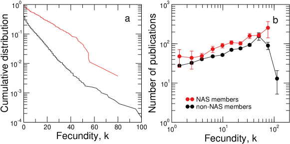
Figure 1: Relationship between mentorship fecundity and other performance metrics. a, Cumulative distribution of the mentorship fecundity for NAS members (red) and non-NAS members (black). NAS members have an average fecundity of $\langle k\rangle_{\rm NAS}=14$, which is far greater than the average fecundity of non-NAS members $\langle k\rangle_{\rm non-NAS}=3.1$, indicating that fecundity is closely related to academic recognition. Note that not all mathematicians in the non-NAS group were elegible for NAS membership due to citizenship and other circumstances. This fact makes the result in the figure all the more striking. b, Average and standard error (symbols and error bars) of the number of publications as a function of the mentorship fecundity for NAS members (red) and non-NAS members (black). NAS members have nearly twice as many publications on average as non-NAS members for all fecundity levels.

Although the mentorship records gathered from the Mathematics Genealogy Project provide the most comprehensive data source available for studying academic performance throughout a mathematician’s career, there are obviously other plausible metrics for evaluating academic performance [20, 21, 22]. We have also compared the mentorship data against a list of publications for 4,447 mathematicians and a list of 269 inductees into the United States’ National Academy of Sciences (NAS) (see Methods). We find that mentorship fecundity is much larger for NAS members than for non-NAS members (Fig. 1a). We further find that the number of publications is strongly correlated with fecundity, regardless of whether or not a mathematician is a NAS member (Fig. 1b). These results demonstrate that, although fecundity is not a typical measure of academic performance, it is closely related to other measures of academic success. Thus, even though our investigation concerns how fecundity is correlated between mentor and protégé, our results also address questions in the academic evaluation literature concerning the success of a mathematician.

We first investigate whether it is possible to predict the fecundity of a mathematician by modeling the fecundity distribution $p\!\left(k|t\right)$ as a function of graduation year $t$. Considering that some mathematicians remain in academia throughout their career while others spend only a portion of their career in academia, one might expect that there are two types of individuals when it comes to academic mentorship fecundity—“haves” and “have-nots”—in the sense that these mathematicians have or have not had the opportunity to mentor students throughout their career. If each mentor chooses to train a new academic protégé with probability $\xi_{h}$ or $\xi_{hn}$ and stops training academic protégés otherwise, depending on whether they are a “have” or “have-not” respectively, then we would expect that the resulting fecundity distribution is a mixture of two discrete exponential distributions

$$p\!\left(k|\boldsymbol{\theta}\right)=\pi_{h}p\!\left(k|\kappa_{h}\right)+(1-\pi_{h})p\!\left(k|\kappa_{hn}\right),$$ (1)

where $\pi_{h}$ is the probability that a mathematician is a “have”, and $p\!\left(k|\kappa_{h}\right)$ and $p\!\left(k|\kappa_{hn}\right)$ are discrete exponential distributions $p\!\left(k|\kappa\right)=e^{-k/\kappa}(1-e^{-1/\kappa})$ with average fecundity $\kappa_{h}=1/\ln\xi_{h}^{-1}$ and $\kappa_{hn}=1/\ln\xi_{hn}^{-1}$ for “haves” and “have-nots” respectively. We estimate the parameters $\boldsymbol{\theta}=\{\pi_{h},\kappa_{h},\kappa_{hn}\}$ of this distribution from the empirical data using expectation-maximization [23]. Using Monte Carlo hypothesis testing (see Methods), we have found that Eq. (1) can not be rejected as a candidate description of the fecundity distribution $p\!\left(k|t\right)$. For an alternative description of the fecundity distribution $p\!\left(k|t\right)$, see Supplementary Discussion and Fig. S1.

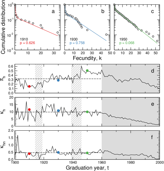
Figure 2: Evolution of the fecundity distribution. a–c, Cumulative distribution of the fecundity of mathematicians that graduated during 1910, 1930, and 1950 (symbols) compared with the best-estimate predictions of a mixture of two discrete exponentials (lines). Monte Carlo hypothesis testing confirms that this model can not be rejected as a model of the fecundity distribution during every year from 1900–1960, as denoted by the P-values above the $\alpha=0.05$ significance level (see Methods). d–f, Best-estimate parameters calculated by maximum likelihood for a mixture of two discrete exponentials as a function of time. Dashed lines denote average parameter values between 1900–1960 and colored circles denote the years displayed in panels a–c. The probability $\pi_{h}$ of being an “have” changes over time, generally corresponding with historic events (hashed grey shading). In contrast, the average fecundities $\overline{\kappa}_{h}=9.8\pm 0.4$ and $\overline{\kappa}_{hn}=0.47\pm 0.03$ remain stable until 1960, at which point they steadily decrease (grey shaded region), corresponding with the time at which mentorship records become incomplete (see Methods).

As one might expect, the probability $\pi_{h}$ that an individual is a “have” experiences dramatic changes over time due to historical events, such as two World Wars, the beginning of the Cold War, and considerable increases in academic funding (Fig. 2b). In contrast, the average fecundities of “haves” and “have-nots” do not exhibit systematic historical changes—$\overline{\kappa}_{h}=9.8\pm 0.4$ and $\overline{\kappa}_{hn}=0.47\pm 0.03$—suggesting that these quantities offer fundamental insight into the mentorship process among mathematicians (Fig. 2c–d).

The stationarity of $\kappa_{h}$ and $\kappa_{hn}$ also provides a simple heuristic for classifying an individual as a “have” or a “have-not”; by maximum likelihood, an individual is a “have” if $k\geq 2$ and a “have-not” otherwise. These results raise the possibility that similar features, perhaps with different characteristic scales of fecundity, may be present in other mentorship domains.

While our description of the fecundity distribution has highlighted a fundamental property of mentorship among mathematicians, it is not predictive of the behavior of individual mathematicians in the sense that fecundity, according to this model, is a random variable drawn from a distribution of Eq. (1). We next test whether protégés mimic the mentorship fecundity of their mentors by comparing protégé fecundity with a suitable null model that does not introduce correlations in fecundity. In analogy with ancestral genealogies and their notion of parents giving birth to children, networks generated from uncorrelated branching processes offer a useful and appropriate context for studying the mathematician genealogy network. Here, a graduation date is equivalent to a birth date and mentors and protégés are equivalent to parents and children, respectively. We will consequently use the subscripts $p$ and $c$ when it is necessary to make generational statements relating parents and children.

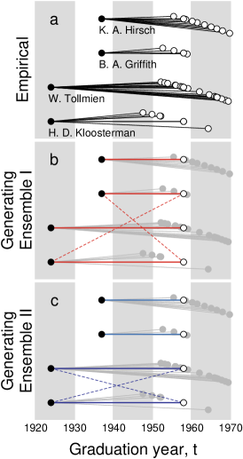
Figure 3: Branching process null models. a, Subset of the mathematician genealogy network. Mentors/parents (black circles) are connected to each of their protégés/children (white circles). The horizontal positions of mathematicians represent their graduation/birth date $t$. The bottom two parents were born in 1924, the top two parents were born in 1937, and all four parents have a child born in 1958. From the parent’s perspective, three essential features of the empirical network must be preserved in random networks generated from the two branching process null models: the birth date $t_{p}$, the fecundity $k_{p}$, and the chronology of child births $\{t_{c}\}$. b, Random networks from Ensemble I preserve these three essential features. Solid lines highlight the links in the empirical network whose end points can be randomized. Dashed lines illustrate one of the possible randomization moves after switching the corresponding pair of links. Note that the age difference between parent and child is not preserved. c, Random networks from Ensemble II preserve these three essential features as well as the age difference between parent and child. Solid lines of the same color highlight the links in the empirical network whose end points can be randomized. Dashed lines illustrate one of the possible randomization moves after switching the corresponding pair of links. Random networks for each ensemble are generated by attempting 100 switches per link (see Methods).

In a branching process [24], a parent $p$, born at time $t_{p}$, has $k_{p}$ children. A child $c$ of parent $p$ is born at time $t_{c}$ and subsequently has $k_{c}$ children. The fecundity $k$ of each individual is drawn from the conditional fecundity distribution $p\!\left(k|t\right)$ for an individual born at time $t$. Networks generated from this type of branching process are therefore defined by the birth date of each individual $t$, the fecundity distribution $p\!\left(k|t\right)$, and the chronology of child births $\{t_{c}\}$ for each parent (Fig. 3a).

We compare the mathematician genealogy network with two ensembles of randomized genealogies from the branching process family. Random networks from Ensemble I retain the birth date of each individual $t$, the fecundity $k$ of each individual, and the chronology of child births $\{t_{c}\}$ for each parent (Fig. 3b). Random networks from Ensemble II additionally restrict parent–child pairs to have the same age difference ($t_{c}-t_{p}$) as parent–child pairs in the empirical network (Fig. 3c). All other attributes of these networks are randomized using a link switching algorithm (see Methods) [25, 26], so neither of these random network ensembles introduces correlations between parent fecundity and child fecundity or temporal correlations in fecundity, providing a suitable basis for comparison with the mathematician genealogy network.

To explore the influence of mentor fecundity and age difference on protégé fecundity, we partition protégés according to the fecundity of their mentors and the age difference between mentor and protégé ($t_{c}-t_{p}$). Given our findings (see Supplementary Discussion, Figs. S2–S3), it is clear that age differences impact fecundity in a non-random manner for protégés whose mentors have $k_{p}<3$. We partition the remaining protégés whose mentors have $k_{p}\geq 3$ into two groups: protégés whose mentors are below-average “haves” ($3\leq k_{p}<10$) and protégés whose mentors are above-average “haves” ($k_{p}\geq 10$). We then partition these three groups of protégés according to when they graduated during their mentors’ career. Specifically, we split each group of protégés into terciles, the most fine-grained grouping that still gives us sufficient power to examine the statistical significance of any differences between the empirical data and the null models.

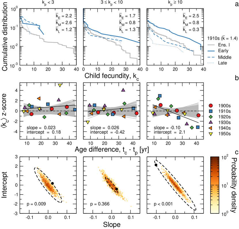
Figure 4: Effect of age difference $t_{c}-t_{p}$ between mentor and protégé on protégé fecundity. a, Fecundity distribution of children born during the 1910s from parents with $k_{p}<3$, $3\leq k_{p}<10$, and $k_{p}\geq 10$ compared with the expectation from Ensemble I (grey line). We separate children into terciles (early, middle, late) according to the time difference in birth dates $t_{c}-t_{p}$ between parents and children. Note that the average fecundity of children born from parents with $k_{p}<3$ is larger than expected, regardless of whether they were born during the early, middle, or later part of their parent’s life. Note also that the average fecundity of children born from parents with $k_{p}\geq 10$ decreases throughout their parent’s life. b, We quantify the significance of these trends during each decade (colored symbols) by computing the $z$-score of the average child fecundity $\langle k_{c}\rangle$ compared with the average child fecundity in networks from Ensemble I. This information is summarized by identifying the linear regression (solid black line). Note that the regression lines for networks from our null model (grey lines) vary around the expectation of our null model (dashed black line). c, Significance of linear regressions in panel b. We compare the slope and intercept of the empirical regression (black circle) with the distribution of the slope and intercept of the same quantities computed from the null model. Since these quantities are approximately distributed as a multivariate Gaussian, we compute the equivalent of a two-tailed P-value by finding the fraction of synthetically generated slope–intercept pairs that lie outside of the equi-probability surface of the multivariate Gaussian (dashed ellipse). Note that the slope and intercept of the regression for children from parents with small ($p=0.009$) and large fecundity ($p<0.001$) are significantly different from the expectation for the null model, consistent with the data displayed in panel a. Comparisons with expectations from random networks from Ensemble II yield the same conclusions (Fig. S4).

We use the partitioning of children into classes to examine the relationship between the average child fecundity $\langle k_{c}\rangle$ and the age difference $t_{c}-t_{p}$ between parent and child (Figs. 4a,b and S4a,b). If the data are consistent with a branching process, then we would expect the average child fecundity $\langle k_{c}\rangle$ to exhibit no temporal dependence. However, the regressions between the average child fecundity $z$-score (see Methods) and the age difference between parent and child $t_{c}-t_{p}$ deviate significantly (Figs. 4c and S4c) from this expectation for both random ensembles to reveal three distinct features. First, mentors with $k_{p}<3$ train protégés that go on to have a 37% larger than expected mentorship fecundity throughout their career. Second, in the first third of their career, mentors with $k_{p}\geq 10$ train protégés that go on to have a 29% larger than expected fecundity. Finally, in the last third of their career, mentors with $k_{p}\geq 10$ train protégés that go on to have a 31% smaller than expected fecundity.

The fact that mentors with $k<3$ train protégés with larger than expected fecundity throughout their career is somewhat counter-intuitive. According to the rising star hypothesis [11, 12], one might have expected that protégés trained by mentors with $k<3$ are likely to mimic their mentors and therefore have smaller than expected fecundity. Our results demonstrate that this is not the case. One possible explanation is that mentors with $k<3$ are more aware of the resources they must allocate for effective mentorship, leading to a more enriching mentorship experience for their protégés. An alternative hypothesis is that mentors with $k<3$ select for, or are selected by, protégés that have a greater aptitude for mentorship.

The striking temporal correlations for mentors with $k_{p}\geq 10$ are intriguing as well. Since mentors with $k_{p}\geq 10$ represent the upper echelon of mentors in mathematics, these mentors are likely “rising stars” early in their academic career. The fact that these mentors train protégés with large fecundity early in their career supports the rising star hypothesis.

By the end of these mentor’s careers, however, their protégés have smaller than expected fecundity. Perhaps mentors, who ultimately have large fecundity, spend less and less resources training each of their protégés as their career progresses. Alternatively, protégés with large mentorship fecundity aspirations might court prolific mentors early in their mentor’s career whereas protégés with small fecundity aspirations might court prolific mentors later in their mentor’s career. Our findings therefore reveal interesting nuances to the rising star hypothesis.

It is unclear whether the temporal correlations we uncover in mentorship fecundity might generalize beyond mathematicians in academia. Anecdotally, mathematicians are thought to perform their best work at a young age [27], a perception that may influence how mentors and protégés choose each other. Perceptions in other domains, however, may differ and subsequently influence mentor and protégé selection in different ways. As data for other academic disciplines [18, 19], business and the government becomes available, it will be important to determine whether temporal correlations in fecundity are a general consequence of mentorship, or a particular consequence of mentorship for mathematicians in academia.

Regardless, our results offer another means of judging academic impact in science as well as the impact of managers on their employees, both of which are notoriously complicated and risky affairs. These assessments are multi-dimensional, metrics and expectations are domain dependent, and placement of creative output, time-scales of impact and recognition vary significantly from field to field. Ultimately, assessment of individuals for awards and promotion is based on painstaking individual analysis by selection committees and peers. While these committees may have varying goals and incentives, it is important that collective arguments—the kind of arguments we are making here—be based on sound quantitative analysis. Although the extent to which our findings extrapolate to other domains may vary, we are confident that the kind of analysis presented here will serve to elevate the discourse on scientific and managerial impact.

Data acquisition. We use data from the Mathematics Genealogy Project [17] to identify the 7,259 protégé mathematicians that are in the giant component [28] and graduated between 1900 and 1960, of which 4,447 of them have linked publication records through MathSciNet. We use a text matching algorithm [29] to semi-automatically match members of the National Academy of Science with mathematicians from the Mathematics Genealogy Project.

Monte Carlo hypothesis testing for $\boldsymbol{p\!\left(k|t\right)}$. We use Monte Carlo hypothesis testing [30] to determine whether Eq. (1) with maximum-likelihood [23] parameters $\boldsymbol{\theta}$ can be rejected as a candidate model for $p\!\left(k|t\right)$ at the $\alpha=0.05$ significance level.

Random network generation. We use a variation of the Markov chain Monte Carlo algorithm [25, 26] to construct each of the 1,000 random networks in Ensembles I and II. Specifically, we restrict the switching of endpoints of links $p\rightarrow c$ that belong to the same link class $\mathcal{L}$, where the link classes are defined as $\mathcal{L}_{\rm I}(t)=\{p\rightarrow c|t_{c}=t\}$ and $\mathcal{L}_{\rm II}(s,t)=\{p\rightarrow c|t_{p}=s,t_{c}=t\}$ for networks from Ensembles I and II, respectively. Each link class $\mathcal{L}$ can be thought of as a subgraph, which can then be randomized in the usual way by attempting 100 switches per link in each link class $\mathcal{L}$ [25, 26].

Average fecundity z-score. By the central limit theorem, the average of variates drawn from $p\!\left(k_{c}|t_{c}\right)$ is normally distributed since $p\!\left(k_{c}|t_{c}\right)$ is well-described by a mixture of discrete exponential distributions, a distribution with finite variance. Given a set of child fecundities $K_{c}=\{k_{c}\}$, we quantify how significantly a subset of these child fecundities $K_{c}^{\ast}\subset K_{c}$ deviates from $K_{c}$ by measuring the $z$-score of the average child fecundity $\langle k_{c}\rangle$ of all nodes within the subset $K_{c}^{\ast}$ compared with the average child fecundity $\langle k_{c}\rangle_{s}$ computed from children within an equivalent subset $K_{c}^{\ast}$ in the synthetic networks. That is, we compute $z=(\langle k_{c}\rangle-\mu)/\sigma$ where $\mu$ is the ensemble average of $\{\langle k_{c}\rangle_{s}\}$ and $\sigma$ is the standard deviation of the ensemble $\{\langle k_{c}\rangle_{s}\}$ over the 1,000 realizations generated for our null models.

is linked to the online version of the paper at www.nature.com/nature.

We thank R. Guimerà, P. McMullen, A. Pah, M. Sales-Pardo, E.N. Sawardecker, D.B. Stouffer, and M.J. Stringer for insightful comments and suggestions. L.A.N.A. gratefully acknowledges the support of NSF awards SBE 0830388 and IIS 0838564. All figures were generated with PyGrace (http://pygrace.sourceforge.net) with color schemes from http://colorbrewer.org.

R.D.M. analyzed data, designed the study, and wrote the paper. J.M.O. and L.A.N.A. designed the study and wrote the paper.

Reprints and permissions information is available at npg.nature.com/reprintsandpermissions. The authors declare that they have no competing financial interests. Correspondence and requests for materials should be addressed to J.M.O. (jm-ottino@northwestern.edu) or L.A.N.A. (amaral@northwestern.edu).

Mathematics Genealogy Project data

We study a prototypical mentorship network collected from the Mathematics Genealogy Project [17], which aggregates the graduation date, mentor, and advisees of 114,666 mathematicians from as early as 1637. From this information, we construct a mathematician genealogy network where links are formed from a mentor to each of his $k$ protégés.

The data collected by the Mathematics Genealogy Project are self-reported, so there is no guarantee that the observed genealogy network is a complete description of the mentorship network. In fact, 16,147 mathematicians do not have a recorded mentor and, of these, 8,336 do not have any recorded protégés. To avoid having these mathematicians distort our analysis, we restrict our analysis to the 90,211 mathematicians that comprise the giant component [28] of the network; that is, we restrict our analysis to the largest set of connected mathematicians in the mathematician genealogy network.

Although the Mathematics Genealogy Project contains information on mathematicians from as early as 1637, this does not necessarily indicate that all of these records are representative of the evolution of the network. For example, prior to 1900, the Project records fewer than 52 new graduates per year worldwide. Furthermore, since mathematicians oftentimes have mentorship careers lasting 50 years or more (Fig. LABEL:fig:graduation_rate), we are not guaranteed to have complete mentorship records for mathematicians that graduated after 1960. We therefore restrict our analysis to the 7,259 protégé mathematicians that graduated between 1900 and 1960, for whom we believe that the graduation and mentorship record is the most reliable.

MathSciNet data

Of the 7,259 protégé mathematicians that graduated between 1900 and 1960, 4,447 of them have linked MathSciNet publication records which are used in our analysis.

U.S. National Academy of Science data

The United States’ National Academy of Science maintains two databases of its membership. The first database consists of all deceased members elected to the Academy from as early as 1863. This database records the name of the inductee, their election year, their date of death, and a link to a biographical sketch. The second database consists of all active members of the Academy. This database records the name of the inductee, their institution, their academic field, and their election year.

The challenge to matching this data with the Mathematics Genealogy Project data is that there is no direct link between a member of the National Academy and Mathematics Genealogy Project page and vice versa. This ambiguity is somewhat confounded by the fact that some members of the Academy have common names. To circumvent these problems, we use a text matching algorithm [29] to semi-automatically detect if a member of the Academy matches a name in the Mathematics Genealogy Project database. We use this procedure to curate the 269 members of the Academy that definitively match mathematicians in the Mathematics Genealogy Project database.

Monte Carlo hypothesis testing for $\boldsymbol{p\!\left(k|t\right)}$

Given a model $\mathcal{M}$ with parameters $\boldsymbol{\theta}_{t}$ for the empirically observed fecundity distribution $p\!\left(k|t\right)$, we use Monte Carlo hypothesis testing to determine whether the model $\mathcal{M}$ can be rejected as a candidate model for $p\!\left(k|t\right)$ [30]. The Monte Carlo hypothesis testing procedure is as follows. First, we calculate the best-estimate parameters $\widehat{\boldsymbol{\theta}}_{t}$ for model $\mathcal{M}$ at time $t$ using maximum likelihood estimation [23]. Second, we compute the test statistic $\mathcal{S}$ (detailed below) between the model $\mathcal{M}(\widehat{\boldsymbol{\theta}}_{t})$ and the empirical fecundity distribution $p\!\left(k|t\right)$. We next generate a synthetic fecundity distribution $p_{s}\!\left(k\right)$ from model $\mathcal{M}(\widehat{\boldsymbol{\theta}}_{t})$ using the best-estimate parameters $\widehat{\boldsymbol{\theta}}_{t}$, and we treat the synthetic data exactly the same as we treated the empirical data: first, we calculate the best-estimate parameters $\widehat{\boldsymbol{\theta}}_{s}$ for model $\mathcal{M}$ from maximum likelihood estimation; second, we compute the test statistic $\mathcal{S}_{s}$ between the model $\mathcal{M}(\widehat{\boldsymbol{\theta}}_{s})$ and the synthetic fecundity distribution $p_{s}\!\left(k\right)$. We generate synthetic fecundity distributions $p_{s}\!\left(k\right)$ and their corresponding synthetic test statistics $\mathcal{S}_{s}$ until we accumulate an ensemble of 1,000 Monte Carlo test statistics $\{\mathcal{S}_{s}\}$. Finally, we calculate a two-tailed P-value with a precision of 0.001. As is customary in hypothesis testing, we reject the model $\mathcal{M}$ at time $t$ if the P-value is less than a threshold value. We select a P-value threshold of 0.05; that is, if less than 5% of the synthetic data sets exhibit deviations in the test statistic that are larger than those observed empirically, the model is rejected at time $t$.

Since we are conducting hypothesis tests with the fecundity distribution $p\!\left(k|t\right)$—a distribution with a discrete support—it is important to use a test statistic $\mathcal{S}$ that is appropriate for testing discrete distributions. We use the $\chi^{2}$ test statistic where we bin $p\!\left(k|t\right)$ such that each bin has at least one expected observation according to the model $\mathcal{M}(\widehat{\boldsymbol{\theta}}_{t})$. This binning prevents observations that are exceptionally rare from dominating our statistical test and skewing our results.

Random network generation

We use Markov chain Monte Carlo algorithm [25, 26] to build random networks from the mathematician genealogy network. The standard version of this algorithm inherently preserves the fecundity of each individual, but it does not preserve the chronology of child births $\{t_{c}\}$ for each parent. To obtain random networks belonging to Ensemble I or Ensemble II, we restrict the switching of endpoints of links $p\rightarrow c$ that belong to the same link class $\mathcal{L}$, where the link classes are defined as $\mathcal{L}_{\rm I}(t)=\{p\rightarrow c|t_{c}=t\}$ and $\mathcal{L}_{\rm II}(s,t)=\{p\rightarrow c|t_{p}=s,t_{c}=t\}$ for networks from Ensembles I and II, respectively. Each link class $\mathcal{L}$ can be thought of as a subgraph, which can then be randomized using the Markov chain Monte Carlo algorithm. Here, we attempt 100 switches per link in each link class $\mathcal{L}$, which sufficiently alters random networks away from the original empirical network [25, 26]. We repeat this procedure 1,000 times to generate a set of 1,000 random networks for each ensemble.

Average fecundity z-score

The average of variates drawn from $p\!\left(k_{c}|t_{c}\right)$ is normally distributed since $p\!\left(k_{c}|t_{c}\right)$ is well-described by a mixture of discrete exponential distributions, a distribution with finite variance, and thus the central limit theorem applies. Given a set of child fecundities $K_{c}=\{k_{c}\}$, we quantify how significantly a subset of these child fecundities $K_{c}^{\ast}\subset K_{c}$ deviates from $K_{c}$ by measuring the $z$-score of the average child fecundity $\langle k_{c}\rangle$ of all nodes within the subset $K_{c}^{\ast}$ compared with the average child fecundity $\langle k_{c}\rangle_{s}$ computed from children within an equivalent subset $K_{c}^{\ast}$ in the synthetic networks. That is, we compute $z=(\langle k_{c}\rangle-\mu)/\sigma$ where $\mu$ is the ensemble average of $\{\langle k_{c}\rangle_{s}\}$ and $\sigma$ is the standard deviation of the ensemble $\{\langle k_{c}\rangle_{s}\}$ over the 1,000 realizations generated for our null models.

References

- [1] Kram, K. E. Mentoring at Work: Developmental Relationships in Organizational Life (Scott Foresman, 1985).
- [2] Chao, G. T., Walz, P. M. & Gardner, P. D. Formal and informal mentorships: A comparison on mentoring functions and contrast with nonmentored counterparts. Personnel Psych. 45, 619–635 (1992).
- [3] Scandura, T. A. Mentorship and career mobility: An empirical investigation. J. Organiz. Behav. 13, 169–174 (1992).
- [4] Aryee, S., Chay, Y. W. & Chew, J. The motivation to mentor among managerial employees. Group Org. Manage. 21, 261–277 (1996).
- [5] Allen, T. D., Poteet, M. L., Russell, J. E. A. & Dobbins, G. H. A field study of factors related to supervisors’ willingness to mentor others. J. Voc. Behav. 50, 1–22 (1997).
- [6] Donaldson, S. I., Ensher, E. A. & Grant-Vallone, E. J. Longitudinal examination of mentoring relationships on organizational commitment and citizenship behavior. J. Career Devel. 26, 233–249 (2000).
- [7] Payne, S. C. & Huffman, A. H. A longitudinal examination of the influence of mentoring on organizational commitment and turnover. Acad. Manage. J. 48, 158–168 (2005).
- [8] Kram, K. E. & Isabella, L. A. Mentoring alternatives: The role of peer relationships in cancer development. Acad. Manage. J. 28, 110–132 (1985).
- [9] Higgins, M. C. & Kram, K. E. Reconceptualizing mentoring at work: A developmental network perspective. Acad. Manage. Rev. 26, 264–283 (2001).
- [10] Allen, T. D., Poteet, M. L. & Burroughs, S. M. The mentor’s perspective: A qualitative inquiry and future research agenda. J. Voc. Behav. 51, 70–89 (1997).
- [11] Green, S. G. & Bauer, T. N. Supervisory mentoring by advisers: Relationships with doctoral student potential, productivity, and commitment. Personnel Psych. 48, 537–561 (1995).
- [12] Singh, R., Ragins, B. R. & Tharenou, P. Who gets a mentor? A longitudinal assessment of the rising star hypothesis. J. Voc. Behav. 74, 11–17 (2009).
- [13] Allen, T. D., Poteet, M. L. & Russell, J. E. A. Protégé selection by mentors: What makes the difference? J. Organiz. Behav. 21, 271–282 (2000).
- [14] Allen, T. D. Protégé selection by mentors: Contributing individual and organizational factors. J. Voc. Behav. 65, 469–483 (2004).
- [15] Ragins, B. R. & Scandura, T. A. Burden or blessing? Expected costs and benefits of being a mentor. J. Organiz. Behav. 20, 493–509 (1999).
- [16] Paglis, L. L., Green, S. G. & Bauer, T. N. Does adviser mentoring add value? A longitudinal study of mentoring and doctoral student outcomes. Res. High. Ed. 47, 451–476 (2006).
- [17] http://genealogy.math.ndsu.nodak.edu (accessed Nov. 2007).
- [18] Bourne, P. E. & Fink, J. L. I am not a scientist, I am a number. PLoS Comput. Biol. 4, e1000247 (2008).
- [19] Enserink, M. Are you ready to become a number? Science 323, 1662–1664 (2009).
- [20] King, J. A review of bibliometric and other science indicators and their role in research evaluation. J. Inf. Sci. 13, 261 (1987).
- [21] Moed, H. F. Citation Analysis in Research Evaluation (Springer, 2005).
- [22] Hirsch, J. E. An index to quantify an individual’s scientific research output. Proc. Natl. Acad. Sci. U.S.A. 102, 16569–16572 (2005).
- [23] Bishop, C. M. Pattern Recognition and Machine Learning (Springer, 2007).
- [24] Athreya, K. B. & Ney, P. E. Branching Processes (Courier Dover Publications, Mineola, New York, 2004).
- [25] Milo, R., Kashtan, N., Itzkovitz, S., Newman, M. E. J. & Alon, U. On the uniform generation of random graphs with prescribed degree sequences. arXiv:cond-mat/0312028.
- [26] Itzkovitz, S., Milo, R., Kashtan, N., Newman, M. E. J. & Alon, U. Reply to “Comment on ‘Subgraphs in random networks’ ”. Phys. Rev. E 70, 058102 (2004).
- [27] Hardy, G. H. A Mathematician’s Apology (University Press, Cambridge, 1940).
- [28] Stauffer, D. & Aharony, A. Introduction to Percolation Theory (Taylor & Francis, 1992), 2nd edn.
- [29] Chapman, B. & Chang, J. Biopython: python tools for computational biology. ACM SIGBIO Newslett. 20, 15–19 (2000).
- [30] D’Agostino, R. B. & Stephens, M. A. Goodness-of-Fit Techniques (Marcel Kekker, Inc., New York, NY, 1986).