Signatures of transition region explosive events in hydrogen Ly$\beta$  profiles

Abstract

Aims. We search for signatures of transition region explosive events (EEs) in hydrogen Ly$\beta$  profiles.

Methods. Two rasters made by the SUMER (Solar Ultraviolet Measurements of Emitted Radiation) instrument on board SOHO in a quiet-Sun region and an equatorial coronal hole are selected for our study. Transition region explosive events are identified from profiles of C ii 1037Å and O vi 1032 Å, respectively. We compare Ly$\beta$ profiles during EEs with those averaged in the entire quiet-Sun and coronal-hole regions. The relationship between the peak emission of Ly$\beta$ profiles and the wing emission of C ii and O vi during EEs is investigated.

Results. We find that the central part of Ly$\beta$  profiles becomes more reversed and the distance of the two peaks becomes larger during EEs, both in the coronal hole and in the quiet Sun. The average Ly$\beta$  profile of the EEs detected by C ii has an obvious stronger blue peak. During EEs, there is a clear correlation between the increased peak emission of Ly$\beta$ profiles and the enhanced wing emission of the C ii and O vi lines. The correlation is more pronounced for the Ly$\beta$  peaks and C ii wings, and less significant for the Ly$\beta$  blue peak and O vi blue wing. We also find that the Ly$\beta$  profiles are more reversed in the coronal hole than in the quiet Sun.

Conclusions. We suggest that the jets produced by EEs emit Doppler-shifted Ly$\beta$ photons, causing enhanced emission at positions of the peaks of Ly$\beta$ profiles. The more-reversed Ly$\beta$  profiles confirm the presence of a larger opacity in the coronal hole than in the quiet Sun. The finding that EEs modify the Ly$\beta$ line profile in QS and CHs implies that one should be careful in the modelling and interpretation of relevant observational data.

1 Introduction

Transition region (TR) explosive events (EEs) are small-scale dynamic phenomena often observed in the far and extreme ultraviolet (FUV/EUV) spectral lines formed in the solar transition region. They were detected for the first time by the NRL/HRTS instrument (Brueckne & Bartoe, 1983). Since 1996, data obtained by the SUMER (Solar Ultraviolet Measurements of Emitted Radiation) spectrograph (Wilhelm et al., 1995, 1997) have been widely used to study EEs. With high spatial and spectral resolution, and wide spectral coverage, SUMER has greatly increased our knowledge of EEs. EEs are characterized by non-Gaussian and broad profiles with enhancements in the blue/red wings with an average line-of-sight Doppler velocities of $\sim$100 km/s (Dere et al., 1989; Innes et al., 1997a). They have a small spatial scale of about 1800 km and a short lifetime of about 60 s on average (Teriaca et al., 2004). Explosive events tend to occur along the boundaries of the magnetic network, where weak mixed-polarity magnetic features are present (Porter & Dere, 1991; Chae et al., 1998; Teriaca et al., 2004). As EEs are often found to be associated with magnetic cancelation and reveal bi-directional flows with high velocities comparable to the local Alfvén velocity, they have been suggested to be a consequence of small-scale magnetic reconnections (Innes et al., 1997b). Sometimes EEs are found to burst repeatedly in the same region, possibly a result of repetitive reconnections triggered by P-mode oscillations or transverse oscillations of the flux tubes (Ning et al., 2004; Doyle et al., 2006; Chen & Priest, 2006). Although EEs are best seen in typical TR lines, they can generally be detected in spectral lines with formation temperatures ranging from $\sim$$10^{4}$ to 5$\times 10^{5}$ K (Madjarska & Doyle, 2002; Teriaca et al., 2002; Popescu et al., 2007).

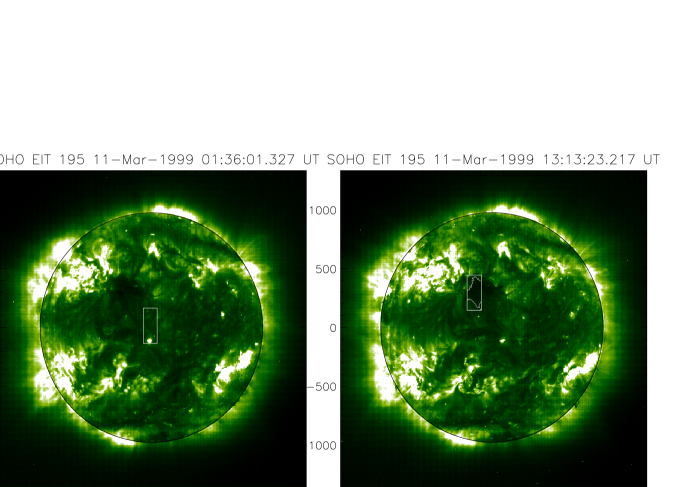
Figure 1: Two EIT images in the 195 Å passband. The white rectangles indicate the scanned regions by SUMER (left: QS right: ECH), the curve on the right image outlines the ECH boundary.

Table 1: Information of the SUMER observations

Date	Time	Solar X	Solar Y	Detector	slit	Exposure time
1999.03.11	01:28-02:25	(-63′′, 67′′)	0′′	A	2	30 s
1999.03.11	12:09-13:09	(-223′′, -88′′)	280′′	A	2	30 s

Hydrogen is the most abundant element in the solar atmosphere and its resonance lines play an important role in the energy transport of the Sun (Fontenla et al., 1988). Ly$\beta$ is the second prominent line in the H Lyman series. Important information on the highly dynamic TR structures may be carried by the profiles of this line. Early rocket and satellite observations obtained some Ly$\beta$  profiles (Reeves, 1976; Lemaire et al., 1978; Vial, 1982). However, the profiles obtained in these early observations suffered from geocoronal absorption. Theoretical models suggested that the reversal at the center of the Ly$\beta$  profiles is formed in the upper chromosphere and lower transition region, while the wings formed in the lower chromosphere (Gouttebroze et al., 1978; Barsi et al., 1979; Schmieder et al., 1998). Recently, the Ly$\beta$ profiles obtained with the SUMER instrument have been extensively investigated. Most Ly$\beta$  profiles appear to have a non-Gaussian shape with a self-reversal at the center and two peaks aside, with different shapes in different regions (Warren et al., 1998; Heinzel et al., 2001; Xia, 2003; Xia et al., 2004; Vial et al., 2007; Schmieder et al., 2007; Curdt et al., 2008; Tian et al., 2009a, b, c; Curdt et al., 2010a). It is believed that the asymmetries of the Ly$\beta$  profiles are probably caused by the combined effect of flows and opacity in different layers of the solar atmosphere (Fontenla et al., 2002; Gunár et al., 2008; Tian et al., 2009b). Higher-order Lyman line profiles were also studied. For example, Warren et al. (1998) found that the average profiles for Ly$\beta$ through Ly$\epsilon$ ($n$=5) are self-reversed and the remaining lines are flat-topped, and Madjarska & Doyle (2002) found that profiles through Ly-6 to Ly-11 reveal self-absorption during EEs. Madjarska & Doyle (2002) suggested that the observed central depression during EEs in Lyman lines may be mainly due to an emission increase in the wings.

Although previous studies have demonstrated that hydrogen Lyman series behave very differently in different solar regions, it is clear that more data need to be analyzed to advance our knowledge. As the second prominent line of the hydrogen Lyman series, Ly$\beta$  has been frequently used in SUMER observations, and can thus provide a valuable tool to diagnose different structures and properties in various solar regions.

In this paper, we use co-temporal observations of O vi, C ii, and Ly$\beta$ in a quiet-Sun region (QS) and an equatorial coronal hole (ECH), to search for signatures of EEs in Ly$\beta$ profiles in these different solar regions. The correlation between the increased peak emission of Ly$\beta$ profiles and the enhanced wing emission of O vi and C ii is investigated and discussed.

2 OBSERVATIONS AND DATA ANALYSIS

Information of the SUMER observations is listed in Table 1. The first data set was taken in the quiet Sun, and the second one was obtained in an equatorial coronal hole. The solar X (East-West) refers to the coordinate range of the scanned region. The solar Y (South-North) refers to the coordinate of the slit center. Each of the data includes O vi (1031.9 Å, $T_{e}\approx 3\times 10^{5}$K), C ii (1037.0 Å, $T_{e}\approx 5\times 10^{4}$K), and H I Ly$\beta$ (1025.7 Å, $T_{e}\approx 2\times 10^{4}$K) lines and a series of full detector readouts at different wavelengths. The scanned regions are outlined by white rectangles and overlapped on the EIT 195 images (see Fig.1).

We applied the standard procedures for correcting and calibrating the SUMER raw data. They include decompression, reversal, flat-field, dead-time, local-gain, and geometrical corrections. We extracted the raster scan coordinates from the head-data files of SUMER and eliminated effects of the solar rotation. The coalignment of images obtained by different instruments was achieved through a cross-correlation between the Ly$\beta$ intensity maps, the EIT images and MDI magnetograms.

EEs were identified by O vi and C ii profiles, respectively. We first used the procedure described in Xia (2003) to deduce the widths of all spectra and calculated the standard deviation of the widths. We disregarded the noisy profiles with a peak intensity smaller than the half-peak intensity of the average profile. Then the profiles with a width larger than three standard deviations (3$\sigma$) were singled out for further visual inspection to finally determine the occurrence of EEs. Our method is similar to those used by Teriaca et al. (2004).

3 RESULTS

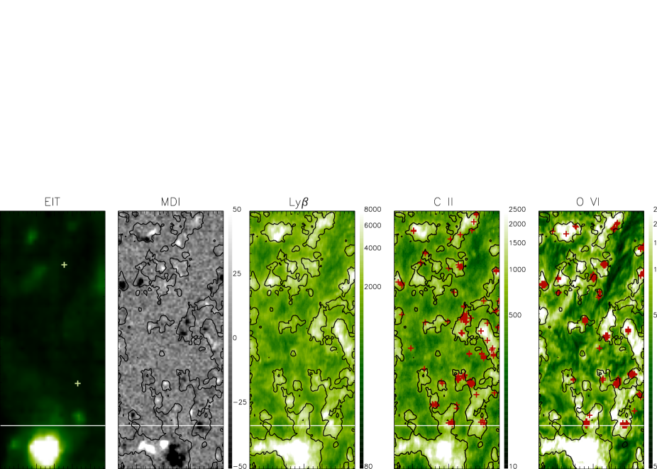
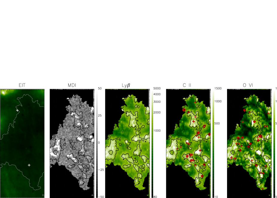
Figure 2: EIT images in the 195 Å passband, magnetograms (unit: G) obtained by MDI, intensity maps (unit: counts/30s/line) of Ly$\beta$ , C ii and O vi (top: QS bottom: ECH). Contours overlaid on the magnetogram and intensity maps of SUMER, obtained from the continuum around 1032 Å, outline the chromospheric network. EEs are marked with the red ’+’ symbols. The ’+’ symbols in EIT images mark locations of four EEs which are analyzed in Fig.3.

Figure 2 shows the EIT images in the 195 Å passband, magnetograms obtained by MDI, intensity maps of Ly$\beta$ , C ii and O vi. In the upper panel, in order to remove the interference of a coronal bright point (seen in the bottom of the EIT map), we used only the region above the horizontal line to calculate the averaged quiet-Sun profiles. In the lower panel, the boundary of the equatorial coronal hole was determined with the intensity threshold of the EIT image (Xia, 2003). The magnetogram, intensity maps of Ly$\beta$ ,C ii and O vi are overlaid by black contours to outline the chromospheric network, which occupies 33% of the whole area and is characterized by the highest intensities of the continuum around 1032 Å. It is clear that the network coincides with the concentration of strong photospheric magnetic fields. In the QS region, strong magnetic fields with positive (white) and negative (black) polarities are both present inside the network, while in the ECH region the network regions are dominated by strong positive magnetic fields and only a few weak mixed-polarity fields are present. The network structures indicated by the continuum intensity coincide well with the strong emission of the three lines. There are many loop-like structures which have visible footpoints lying on the edge of networks and extend into the cell interiors. The loop-like structures can be identified much easier in the ECH than in the QS. A more detailed discussion about the morphology in these two regions can be found in Xia et al. (2004).

Explosive events are best seen in typical transition-region lines like Si iv($T_{e}\approx 8\times 10^{4}$ K), they can generally be detected in spectral lines with formation temperatures ranging from $\sim$10⁴ to 5$\times$10⁵ K (Madjarska & Doyle, 2002; Teriaca et al., 2002; Popescu et al., 2007). Here we use two transition-region lines C ii and O vi, respectively, to identify EEs. The identified events are referred to as “C ii EEs” and “O vi EEs” hereinafter. In Fig. 2, the red ’+’ in intensity maps of C ii and O vi mark locations of pixels where EEs were identified. We find 136 EE pixels detected by the C ii line and 167 by the O vi line in the QS, and 70 and 78 correspondingly in the ECH. Neighboring EE pixels in each spectral line are regarded as given by a single event. The average occurrence rates of EEs in both regions are then estimated to be about 1$\times 10^{-20}cm^{-2}s^{-1}$, which is comparable to that obtained by Teriaca et al. (2004) in a QS region. It is clear that most of the EEs lie in the network or on the edge of the network, in line with previous studies. Furthermore, it is interesting to find that the pixel positions of the EEs observed in the C ii and O vi lines are not spatially overlaid with each other in most cases. However, this doesn’t mean that there is no connection between these two lines during the events. By inspection of detailed line profiles, when an EE detected only in one spectral line (i.e., with the line width wider than 3$\sigma$), the other one recorded in the same spectral window at the same location often responses simultaneously and reveals a significant non-Gaussian profile although its line width is still smaller than 3$\sigma$. Note that the formation temperature of the C ii line is about 5 $\times 10^{4}$ K which is an order lower than that of the O vi line. This difference of line temperature may result in a different spectral response to an EE. The response may depend on the height where an EE occurs. A time delay may also exist in the response of the high temperature line with respect to the lower temperature line, if an EE bursts at a lower height.

Figure 3: O vi, Ly$\beta$ , C ii profiles of four EEs (marked in the EIT images of Fig. 2). Thin lines show the average profiles in the QS and ECH. Dotted-lines represent the enhanced radiation by subtracting the mean profiles from the EE profiles.

We selected four individual EEs at different locations detected simultaneously by both the C ii and O vi lines (two in QS and two in ECH, two dominated by red peak and two by blue peak). These EEs are marked on the EIT images shown in Fig.2. In Fig.3, we present EE profiles of the three lines including O vi, Ly$\beta$ and C ii (shown by thick lines), as well as the mean profiles in the whole QS and ECH (shown by thin lines). The emission enhancements in the wings of the O vi and Ly$\beta$ lines are better revealed in the dotted lines which are given by subtracting the mean profiles from the EE ones. We find that during the EEs, velocities of the order of 50-100 km/s are clearly present on the O vi line wings, while the C ii line presents a significant bursting feature. Note that we can only plot the profiles with Doppler velocity of $\pm 80$ km/s for the C ii line due to the presence of another two lines (C ii at 1036.3Å  and O vi at 1037.6Å). It can be seen that the corresponding Ly$\beta$ profiles behave rather differently with a stronger enhancement at the wings and a deeper reversal at the center. In most cases, the distance of the two peaks of Ly$\beta$ profiles is apparently larger than that of the mean Ly$\beta$  profiles, and the intensity and position of the wing peaks of the Ly$\beta$ line correlate well with those of the O vi line (shown by dotted lines). For the three events shown in the first, third and fourth rows of Fig.3, their Ly$\beta$ profiles show very small change of intensity in the line center compared to the mean profile, although their wings enhance very strongly. Note that the above descriptions are only for the four selected individual events detected simultaneously with both the O vi and C ii lines. The more general properties of the observed events will be analyzed below.

Figure 4: Different kinds of average O vi, Ly$\beta$  and C ii profiles (left column: O vi, middle column: Ly$\beta$, right column: C ii; top panels: ECH, bottom panels: QS). Thin solid line is the average profile of each region of entire ECH and QS. Thin dash-dotted, thin dotted and thin dashed lines represent profiles averaged in the top 33%, lower 33%, and intermediate-Ly$\beta$-radiation regions, respectively. Thick solid line shows the average profile of EEs detected by the O vi line and thick dashed line by the C ii line. See also the legend in the top-left panel.

Figure 4 shows different kinds of average O vi, Ly$\beta$ and C ii profiles observed in the QS and ECH regions. The dashed-vertical lines in each panel indicate the central position of the profile averaged in the relevant QS or ECH region. According to the intensity of the Ly$\beta$ line, we divided each region of ECH and QS into three parts: top 33%, lower 33%, and intermediate-radiation regions. Then we calculated the average O vi, Ly$\beta$ and C ii profiles in each radiation region. We find that the red peak of Ly$\beta$  profile is higher than the blue peak in the QS, and the trend becomes more apparent with increasing intensity of Ly$\beta$(seen in bottom panels). In the ECH, the self reversal at the center of the Ly$\beta$  profile is obvious and a deeper one is observed with increasing intensity, while the strengths of two peaks are basically the same (seen in top panels).

In Fig. 4, we also plot the average O vi, Ly$\beta$ and C ii profiles of the O vi EEs (shown by thick solid lines) and the C ii ones (shown by thick dashed lines), respectively. It can be seen that the average Ly$\beta$ profiles of the EEs in both ECH and QS regions show a deeper self-reversal and two prominent wing peaks, and the trend is more obvious for the C ii EEs than the O vi ones. In the ECH, compared with the mean ECH profile(shown by thin solid lines), the average O vi profile of the O vi EEs has a broader width and is shifted towards the blue side, while that of the C ii EEs is not very different. The C ii line of the O vi EEs is on average broader than that of the mean ECH profile, and that of the C ii EEs is even broader. They both tend to have a more enhanced blue wing. And again, the blue wing of the C ii EEs is more enhanced than that of the O vi ones. For the Ly$\beta$  line, the average profile of the O vi EEs is almost symmetric and that of the C ii EEs has an obviously stronger blue peak. The distances of the two peaks observed in both the O vi EEs and C ii EEs are larger than that of the mean ECH profile, and that for the C ii EEs is the largest. In the QS, similar trends can be found for the widths of the C ii and O vi lines. However, the C ii profile of the O vi EEs shows a more enhanced red wing, which may be at least partly caused by the greatly enhanced blue wing of another O vi line at 1037.6Å. And, for the Ly$\beta$ line, the red peak is stronger in the QS, in contrast with the features observed in the ECH. The distance of the two peaks in the QS also shows a similar trend as that in the ECH.

Figure 5: Relationship between photon counts of blue/red wing of O vi and C ii profiles and photon counts of blue/red peak of Ly$\beta$ profiles during EEs. The correlation coefficient is shown in each panel (upper two panels: QS; bottom two panels: ECH)

Table 2: Correlation coefficients of enhanced emission during EEs

correlated parameters	O vi EEs		C ii EEs
	red	blue	red	blue
QS (O vi wing $\sim$ Ly$\beta$  peak)	0.74	0.37	0.77	0.51
QS (C ii wing $\sim$ Ly$\beta$  peak)	0.60	0.60	0.76	0.63
CH (O vi wing $\sim$ Ly$\beta$  peak)	0.70	0.36	0.36	0.34
CH (C ii wing $\sim$ Ly$\beta$  peak)	0.83	0.72	0.72	0.76

In order to quantify the correlation between the increased peak emission of Ly$\beta$ profiles and the enhanced wing emission of O vi, we calculated the photon counts of blue/red wing (Doppler velocity from 30 km/s to 100 km/s) of O vi profiles and the photon counts of blue/red peak (Doppler velocity from 30 km/s to 70 km/s ) of Ly$\beta$ profiles at EE pixels in the QS and ECH, respectively. In the same way, we also calculated the correlation coefficients between the C ii wings (Doppler velocity from 30 km/s to 70 km/s) and the Ly$\beta$ peaks. Figure 5 presents the corresponding scatter plots. We also list the calculated correlation coefficients in Table 2, which are all positive. It seems that the enhancement of the Ly$\beta$ peaks represents the signature of EEs. Furthermore, the correlation seems to be quite good for all red/blue wings of C ii profiles and all red wings of O vi profiles. For the O vi line, the correlation seems to be weaker on the blue than the red side. Note that the formation temperature of the C ii line is much closer to that of the Ly$\beta$ line than that of the O vi line. This may explain the better correlation between the increased peak emission of the Ly$\beta$ line and the enhanced C ii wings during EEs.

4 DISCUSSION

The major finding of this paper is that there is a clear correlation between the increased peak emission of Ly$\beta$ profiles and the enhanced wing emission of the transition-region lines, especially the C ii line, which has a formation temperature close to that of the Ly$\beta$  line. This result indicates that EEs can greatly modify Ly$\beta$ profiles, especially the two peaks of the profiles. The clear correlation suggests that EEs are responsible for the enhanced peak emission of Ly$\beta$.

We can assume that the Ly$\beta$ emission during EEs has two components, the background emission and the jet emission. The former is the emission from the background QS or CH. Its source lies in the upper chromosphere and lower TR. As it propagates to the upper atmosphere, emission from the central part of the profile is absorbed by the atomic hydrogen, revealing a central depression in the profile. On the other hand, the jet emission is largely different. Jets produced by EEs can heat the relatively cold background plasma causing enhanced ionization and further emission in the whole profile of colder lines. This is confirmed by the jet emission of C ii shown in Fig.3. At the same time, the plasma can also be accelerated to a much higher velocity causing greatly enhanced emission in their line wings. Since the jets are usually bidirectional with a high speed, the Ly$\beta$ photons emitted by the jets should also be Doppler-shifted towards both longer and shorter wavelengths. If the speed of the jets has a line-of-sight component, we should observe these Doppler-shifted Ly$\beta$ emission which is added to the almost-at-rest background Ly$\beta$ emission, causing enhancement of the peaks of the background Ly$\beta$ profiles. The jet-emitted Ly$\beta$ profiles experience much less radiative transfer process. This is because that the EEs are most prominent in the middle and upper TR, above which the density is very low and the atomic hydrogen can not significantly absorb the emission from below. Also, the almost rest coronal atmosphere could not absorb the Doppler-shifted jet emission due to the lack of the wavelength match.

Madjarska & Doyle (2002) found that profiles through Ly-6 to Ly-11 reveal self-absorption during EEs. The authors concluded that the observed central depression during EEs in Lyman lines may be mainly due to an emission increase in the wings. Our analysis of the Ly$\beta$ profiles during EEs suggests that the jets produced by EEs emit Doppler-shifted Ly$\beta$ photons and cause enhanced emission at the peaks of Ly$\beta$ profiles. Our result complements that in Madjarska & Doyle (2002). In addition, most previous studies on EE-like dynamic events were conducted based on analysis of optically-thin spectral lines (such as Si IV and O VI lines). Our result further indicates that Ly$\beta$ and other Lyman lines could be used to identify these transient events even in absence of strong spectral lines in the transition region. Since Ly$\beta$ is the second prominent line in the hydrogen Lyman series and is much more frequently used in observations, the variation of the Ly$\beta$ profiles provides a good tool to diagnose different structures and properties in different regions. Our finding of the signatures of EEs in Ly$\beta$ profiles is thus helpful to investigate the thermodynamics of the jets produced by EEs.

The average Ly$\beta$ profiles of EEs have an obviously stronger red peak in the QS, while in the ECH the blue peak seems to be stronger for the C ii EEs. The different relative strengths of the blue-shifted and red-shifted jet-components might account for the different asymmetries. In Section 3, we have discussed the average line widths of EE pixels and found the C ii profile of the C ii EEs in the ECH has an enhanced blue wing being more pronounced than other profiles. Correspondingly, the blue peak of Ly$\beta$ is relatively stronger and the peak separation is larger. The blue-shift of EEs may cause the relatively significant blue peak of Ly$\beta$ profiles. As we know, fast bidirectional jets can lead to the separation of the two peaks. From line profiles of the four typical EEs, we suggest that the different asymmetry of Ly$\beta$ profiles seems to be a result of different speed and strength of EEs’ jets.

In the quiet Sun, most Ly$\beta$ profiles are found to have a stronger red peak (Warren et al., 1998). In fact, the Ly$\beta$ profile has different shapes in different regions. Xia (2003) and Xia et al. (2004) found that there are more Ly$\beta$ profiles with a stronger blue peak in equatorial coronal holes than in the quiet Sun, so that the red-peak asymmetry of the average Ly$\beta$ profile is less pronounced in the ECH. Tian et al. (2009b) found that Ly$\beta$ profiles in polar coronal hole have a stronger blue-peak which is opposite to those in the QS. Here we find that the average Ly$\beta$ profile in the ECH has almost symmetrical peaks. The different asymmetries of the Ly$\beta$ profiles might reflect different flow fields of the upper solar atmosphere in different parts of the Sun. The most prominent difference of systematic flow systems between the polar coronal hole and quiet-Sun regions is that upflows are predominant in the upper TR of polar coronal holes (Dammasch et al., 1999; Hassler et al., 1999; Tu et al., 2005; Tian et al., 2010), while upflows are localized at network junctions in the upper TR of the quiet Sun (Hassler et al., 1999; Tian et al., 2008, 2009d). In ECHs, the flow pattern in the upper TR might be similar to that of the polar coronal hole but the magnitude of the upflows might be smaller (Xia et al., 2003; Aiouaz et al., 2005; Raju, 2009). So the average Ly$\beta$ profile in the ECH reveals an almost symmetrical shape, in an intermediate phase between the red-peak-dominance in the quiet Sun and blue-peak-dominance in polar coronal holes. Another possibility might come from the larger opacity in the coronal hole. Our data reveals that the Ly$\beta$ profiles are on average more reversed in the the ECH than in the QS, which indicates that the opacity is larger in the ECH. This finding complements the previous finding of a larger opacity in polar coronal holes than in the quiet Sun (Tian et al., 2009b). We may assume that the Ly$\beta$ line behaves more or less similar to typical TR lines in the quiet Sun. In polar coronal holes, the opacity is so large that the Ly$\beta$ line now behaves more similar to Ly$\alpha$ , with a stronger blue peak (Curdt et al., 2010b). If the opacity in the ECH is larger than that in the QS but smaller than that in the polar coronal holes, then it is not surprising to observe the almost symmetrical Ly$\beta$ profile in the ECH.

The average and four typical Ly$\beta$ profiles imply the contribution from the wings of EEs. We qualitatively analyzed the relevance between the wings of EEs and peaks of Ly$\beta$ profiles. The relevance between C ii wings of EEs and Ly$\beta$ peaks is very significant, but for the O vi line, the relevance between blue wings of EEs and blue peaks is genenally poorer than that between their red counterparts, especially in the ECH. As we know, C ii has a formation temperature close to that of Ly$\beta$, which is about an order lower than that of O vi. During EEs, it seems that in general, the variation of Ly$\beta$ peaks correlates more closely with that of C ii. However, the scan data used here have no information of time. A larger error appears if the time difference exists among the different lines which are emitted in different layers of the solar atmosphere when EE occurs, especially when we are using the scan data with larger exposure time. For example, Madjarska & Doyle (2002) have observed a time delay of about 20-40 s in the response of the transition-region line (S VI, 200 000K) with respect to the chromospheric line (H I Ly 6, 20 000K), when an EE can be seen in a chromospheric line. Therefore, this conclusion should be verified in the future by analyzing more data, especially time-series data with short exposure times.

Previous studies have confirmed that the line shapes of Ly$\alpha$ and Ly$\beta$ were significantly affected by quasi-steady flow field in the transition region (Curdt et al., 2008; Tian et al., 2009a). In this paper, we find the Ly$\beta$ profiles are also modified by the transient flow field generated by EEs in QS and ECH. This finding implies that one should be careful in the modelling and interpretation of such observational data. According to our results, Lyman profiles, especially when observed at a high spatial and temporal resolution, are affected by both EEs and opacity. When the underlying dynamic process of the solar atmosphere is analyzed by using Ly$\beta$ and other Lyman lines, one should consider not only the line source function and opacity, but also the flow field in the transition region, including both the quasi-steady and transient flows. For instance, one needs to take all these factors into account for the numerical simulation in order to explain the observed line shapes of Lyman series and their relation with the flow field.

The Ly$\beta$ line is the second strongest line of hydrogen Lyman series. Some observational features of this line are similar to those of Ly$\alpha$, while some are very different. The opacity of Ly$\alpha$ is much larger than that of Ly$\beta$. It is interesting to ask whether there are similar behaviours of Ly$\alpha$ profile during EEs, which needs to be addressed in the future. Since hydrogen is the most abundant component of the Sun and Ly$\alpha$ is the most prominent line emitted by the chromosphere and lower transition region, such studies could thus be important for the future high-resolution observations of Lyman lines. Moreover, it is also interesting to look for signatures of other solar dynamic events (such as flares and CMEs) in Lyman lines in order to study these dramatic eruptions. As the formation height of Lyman lines in the solar atmosphere is relatively low, their response to the events could be used to study the initiations of these eruptions and to advance the predicting technology of the associated space weather events.

5 CONCLUSION

We have used co-temporal observations of O vi, C ii and Ly$\beta$ in a quiet-Sun region and an equatorial coronal hole to search for signatures of explosive events in Ly$\beta$ profiles. We find that EEs have significant impacts on the profiles of Ly$\beta$. During EEs, the center of Ly$\beta$  profiles becomes more reversed and the distance of the two peaks becomes larger, both in the equational coronal hole and in the quiet Sun. The average Ly$\beta$  profile of the EEs detected by C ii has an obvious stronger blue peak. Statistical analysis shows that there is a clear correlation between the increased peak emission of Ly$\beta$ profiles and the enhanced wing emission of C ii and O vi. The correlation is more obvious for the Ly$\beta$  peaks and C ii wings, and less significant for the Ly$\beta$  blue peak and O vi blue wing. It indicates that the jets produced by EEs emit Doppler-shifted Ly$\beta$ photons, causing enhanced emission at positions of the peaks of Ly$\beta$ profiles. The more-reversed Ly$\beta$  profiles confirm the presence of a larger opacity in the coronal hole than in the quiet Sun.