Kondo Quantum Criticality of Magnetic Adatoms in Graphene

Abstract

We examine the exchange Hamiltonian for magnetic adatoms in graphene with localized inner shell states. On symmetry grounds, we predict the existence of a class of orbitals that lead to a distinct class of quantum critical points in graphene, where the Kondo temperature scales as $T_{K}\propto|J-J_{c}|^{1/3}$ near the critical coupling $J_{c}$ , and the local spin is effectively screened by a super-ohmic bath. For this class, the RKKY interaction decays spatially with a fast power law $\sim 1/R^{7}$. Away from half filling, we show that the exchange coupling in graphene can be controlled across the quantum critical region by gating. We propose that the vicinity of the Kondo quantum critical point can be directly accessed with scanning tunneling probes and gating.

Graphene is a single atomic sheet of carbon atoms with elementary electronic quasiparticles that behave as massless Dirac fermionsNovo . The Kondo effect has been recently observed in graphenemanoharan ; Chen , and the formation of a Kondo screening cloud around a magnetic adatom is quantum critical at half fillingfradkin90 ; Zhang , crossing over at weak coupling to the standard Fermi liquid case, when the DOS is locally restored by disorderHentschel or gating effectsSengupta . The Kondo resonance in graphene is also strongly sensitive to the position of the adatom in the honeycomb lattice, where the interplay of orbital and spin degrees of freedom may give rise to an SU(4) Kondo effectWehling2 .

In this letter, after establishing a generic one-level exchange interaction Hamiltonian for magnetic adatoms in graphene, we show there is a symmetry class of orbitals in which quantum interference between the different hybridization paths leads to a fixed point where the Kondo temperature $T_{K}\propto|J-J_{c}|^{\nu}$, scales with the mean field exponent $\nu=1/3$, with $J$ as the Kondo coupling near criticality. In the $\nu=1/3$ class, graphene behaves as a super-ohmic bath for the local spin and the RKKY interaction is strongly suppressed, decaying spatially with a fast power law $\sim 1/R^{7}$. Furthermore, we show that the exchange coupling in graphene can be controlled by gating. This effect opens the possibility of exploring the proximity to the Kondo quantum critical point (QCP) in graphene directly with scanning tunneling probe (STM) measurementsUchoa09 ; Zhuang ; sengupta2 ; Wehling .

We start from the graphene Hamiltonian, $\mathcal{H}_{g}=-t\sum_{\sigma,\langle ij\rangle}a_{\sigma}^{\dagger}(\mathbf{R}_{i})b_{\sigma}(\mathbf{R}_{j})+{\rm h.c.},$ where $a,b$ are fermionic operators on sublattices $A$ and $B$, respectively, $t\sim 2.8$ eV is the nearest neighbors hopping energy and $\sigma=\uparrow\downarrow$ labels the spin. In the momentum space,

$$\mathcal{H}_{g}=-t\sum_{\mathbf{p}\sigma}\phi_{\mathbf{p}}a_{\sigma,\mathbf{p}}^{\dagger}b_{\sigma,\mathbf{p}}+h.c.,$$ (1)

where $\phi_{\mathbf{p}}=\sum_{i=1}^{3}\mbox{e}^{i\mathbf{p}\cdot\mathbf{a}_{i}}$, and $\mathbf{a}_{1}=\hat{x}$, $\mathbf{a}_{2}=-\hat{x}/2+\sqrt{3}\hat{y}/2$, and $\mathbf{a}_{3}=-\hat{x}/2-\sqrt{3}\hat{y}/2$ are the lattice nearest neighbor vectors.

In the presence of a localized level, the problem is described by the single impurity Anderson Hamiltoniananderson61 ; Uchoa08 , $\mathcal{H}=\mathcal{H}_{g}+\mathcal{H}_{f}+\mathcal{H}_{U}+\mathcal{H}_{V}$, where $\mathcal{H}_{f}=\sum_{\sigma}\epsilon_{0}\,\hat{n}_{f,\sigma}$ is the Hamiltonian of the localized electrons, with $\hat{n}_{f,\sigma}=f_{\sigma}^{\dagger}f_{\sigma}$ as the number operator, and $\epsilon_{0}$ is the energy of the local state measured relative to the Dirac point, $\mathcal{H}_{U}=U\hat{n}_{f,\uparrow}\hat{n}_{f,\downarrow}$ gives the electronic repulsion in the localized level, and $H_{V}$ describes the hybridization between the local level and the graphene electrons.

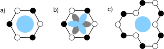
Figure 1: Representation of (a) an $s$-wave and (b) an $f$-wave orbital, when the adatom sits in the center of the graphene honeycomb hexagon. (c) Substitutional impurity in a single vacancy. In the three cases, the adatom hybridizes equally with the neighboring carbons on the same sublattice.

The adatoms in graphene can sit for instance on top of a carbon atom, where the hybridization Hamiltonian is $\mathcal{H}_{V}^{A}\!=\!V\sum_{\sigma}a_{\sigma}^{\dagger}(0)f_{\sigma}+h.c.$, or in the hollow site in the center of the honeycomb hexagon, where the adatom hybridizes with the two sublattices, $\mathcal{H}_{V}^{H}\!=\!\sum_{\sigma}\sum_{i=1}^{3}\left[V_{a,i}a_{\sigma}^{\dagger}(\mathbf{a}_{i})+V_{b,i}b_{\sigma}^{\dagger}(-\mathbf{a}_{i})\right]f_{\sigma}+h.c.$, with $V_{x,i}$ ($x=a,b$) representing the hybridization strength of the localized orbital with each of the three surrounding carbon atoms sitting on a given sublattice. In momentum representation Uchoa09 ,

$$\mathcal{H}_{V}=\sum_{\mathbf{p}\sigma}\left[V_{b,\mathbf{p}}b_{\sigma,\mathbf{p}}^{\dagger}+V_{a,\mathbf{p}}^{*}a_{\sigma,\mathbf{p}}^{\dagger}\right]f_{\sigma}+h.c.\,,$$ (2)

where $V_{a\mathbf{p}}\equiv V\,,$ and $V_{b,\mathbf{p}}=0$ for a top carbon site, say on sublattice $A$ ($A$-site). When the adatom sits in the center of the hexagon ($H$-site), or else for a substitutional impurity in a single vacancykras ($S$-site), the hybridization function is $V_{x,\mathbf{p}}=\sum_{i=1}^{3}V_{x,i}\mbox{e}^{i\mathbf{p}\cdot\mathbf{a}_{i}}.$ On $H$-sites, for an $s$-wave orbital, $V_{x,i}\equiv V$, giving $V_{x,\mathbf{p}}\equiv V\phi_{\mathbf{p}}$, whereas for an in-plane $f$-wave orbital, as shown in Fig. 1b, where the orbital is odd in the two sublattices, $V_{b,i}=-V_{a,i}\equiv V$, resulting in $-V_{a,\mathbf{p}}=V_{b,\mathbf{p}}\equiv V\phi_{\mathbf{p}}$. In the case of an $s$ or in-plane $f$-wave orbital on an $S$-site on sublattice $A$, $V_{a,\mathbf{p}}=0$, and $V_{b,\mathbf{p}}\equiv V\phi_{\mathbf{p}}$, whereas for a substitutional impurity on a $B$-site, $V_{a,\mathbf{p}}\equiv V\phi_{\mathbf{p}}$, and $V_{b,\mathbf{p}}=0$ (see Fig. 1c).

Diagonalizing the non-interacting part of the Hamiltonian $\mathcal{H}$ in the $A$, $B$ sublattices,

$$\mathcal{H}_{g}=\sum_{\mathbf{p}\alpha\sigma}\,E_{\alpha}(\mathbf{p})c_{\alpha,\sigma,\mathbf{p}}^{\dagger}c_{\alpha,\sigma,\mathbf{p}}\,,$$ (3)

where $E_{\alpha}(\mathbf{p})=\alpha t|\phi_{\mathbf{p}}|$ is the graphene tight-binding spectrum, with $\alpha=\pm$ labeling the conduction and valence bands, and $c_{\pm,\sigma,\mathbf{k}}=(b_{\sigma,\mathbf{k}}\pm\phi_{\mathbf{k}}^{*}/|\phi_{\mathbf{k}}|a_{\sigma,\mathbf{k}})/\sqrt{2}$ are the new operators in the diagonal basis. The hybridization term in the rotated basis is

$$\mathcal{H}_{V}=V\sum_{\alpha=\pm}\sum_{\mathbf{p},\sigma}\left[\Theta_{\alpha,\mathbf{p}}c_{\alpha,\mathbf{p}\sigma}^{\dagger}f_{\sigma}+h.c.\right],$$ (4)

where

$$\Theta_{\alpha,\mathbf{p}}=(V_{b,\mathbf{p}}+\alpha V_{a,\mathbf{p}}^{*}\phi_{\mathbf{p}}^{*}/|\phi_{\mathbf{p}}|)/(\sqrt{2}V).$$ (5)

In particular, $\Theta_{\alpha,\mathbf{p}}^{A}=1/\sqrt{2}$ when the adatom is on top of an $A$-site, $\Theta_{\alpha,\mathbf{p}}^{B}=\alpha\phi_{\mathbf{p}}^{*}/(\sqrt{2}|\phi_{\mathbf{p}}|)$ on a $B$-site, and $\Theta_{\alpha,\mathbf{p}}^{H,\gamma}=[\phi_{\mathbf{p}}+(-1)^{\gamma}\alpha\phi_{\mathbf{p}}^{*2}/|\phi_{\mathbf{p}}|]/\sqrt{2}$ when the adatom sits on an $H$-site, where $\gamma=0$ for an $s$-wave orbital and $\gamma=1$ in-plane $f$-wave orbital. In the substitutional case, $\Theta_{\alpha,\mathbf{p}}^{S_{A}}=\phi_{\mathbf{p}}/\sqrt{2}$ for an impurity on sublattice $A$, and $\Theta_{\alpha,\mathbf{p}}^{S_{B}}=\alpha\phi_{\mathbf{p}}^{*2}/(|\phi_{\mathbf{p}}|\sqrt{2})$ on sublattice $B$.

For all possible symmetries, the orbitals of adatoms sitting on $S$ or $H$ sites can be classified among those that either break or preserve the $C_{3v}$ point group symmetry of the triangular sublattice in graphene. Since $|\phi_{\mathbf{p}}|$ scales with $|\omega|/t$, the orbital level broadening, $\Delta(\omega)=\pi V^{2}\sum_{\alpha,\mathbf{p}}|\Theta_{\alpha,\mathbf{p}}|^{2}\delta(\omega-\alpha t|\phi_{\mathbf{p}}|)$ is either $\Delta(\omega)\propto V^{2}\rho(\omega)$ for orbitals that explicitly break the $C_{3v}$ point group symmetry, in which case $|\Theta_{\alpha,\mathbf{p}}|$ scales to a constant near the Dirac points, where $\rho\propto|\omega|$ is the graphene density of states (DOS), or else $\Delta(\omega)\propto V^{2}\rho(\omega)|\omega|^{2}/t^{2}$, for $C_{3v}$ invariant orbitals, when $|\Theta_{\alpha,\mathbf{p}}|\propto|\phi_{\mathbf{p}}|$ scales to zero at small energy. The first class of orbitals, where $\Delta(\omega)\propto|\omega|$ (say, type I), represents the standard case of ohmic dissipationleggett , and is described for instance by adatoms on top carbon sites, by $E_{1}$($d_{xz},$$d_{yz}$) and $E_{2}$$(d_{xy},d_{x^{2}-y^{2}})$ representations of $d$-wave orbitals and $f_{xz^{2}}$, $f_{yz^{2}}$, $f_{xyz}$, $f_{z(x^{2}-y^{2})}$ orbitals in $H$/$S$ sites. The second class, where $\Delta(\omega)\propto|\omega|^{3}/t^{2}$ (type II), represents a new class of super-ohmic dissipationleggett , and is described by $s$, $d_{zz}$, $f_{z^{3}}$, $f_{x(x^{2}-3y^{2})}$, and $f_{y(3x^{2}-y^{2})}$ orbitals in $H$ or $S$ sites (see Fig.1), where the adatom hybridizes equally with the three nearest carbon atoms on a given sublattice. On physical grounds, this new class emerges from quantum mechanical interference between the different hybridization paths in the honeycomb lattice, as the electrons hop in and out of the localized level. As we will show, these two classes of orbitals are described by two distinct types of Kondo QCP.

The Anderson Hamiltonian in graphene can be separated in two terms, $\mathcal{H}=\mathcal{H}_{0}+\mathcal{H}_{V}$, and then mapped into a spin exchange Hamiltonian through a standard canonical transformation, $\bar{\mathcal{H}}=\mbox{e}^{S}\mathcal{H}\mbox{e}^{-S}=\mathcal{H}+[S,\mathcal{H}]+\frac{1}{2}[S,[S,\mathcal{H}]]+...\,$, where $S=-\sum_{\mathbf{p},\alpha\sigma}V[(1-\hat{n}_{f,-\sigma})(\epsilon_{0}-\alpha t|\phi_{\mathbf{p}}|)^{-1}+\hat{n}_{f,-\sigma}(\epsilon_{0}+U-\alpha t|\phi_{\mathbf{p}}|)^{-1}]\Theta_{\alpha,\mathbf{p}}c_{\alpha,\mathbf{p}\sigma}^{\dagger}f_{\sigma}-h.c.\,,$ which results in a Hamiltonian that is quadratic in $V$ to leading order, $\bar{\mathcal{H}}=\mathcal{H}_{0}+[S,\mathcal{H}_{V}]/2+O(V^{3})$Schrieffer . At large $U$, the exchange Hamiltonian is given by

$$\mathcal{H}_{e}=-J\sum_{\mathbf{k}\mathbf{k}^{\prime}}\sum_{\alpha\alpha^{\prime}}\Theta_{\alpha\mathbf{k}}^{*}\Theta_{\alpha^{\prime}\mathbf{k}^{\prime}}\,\mathbf{S}\cdot c_{\alpha^{\prime},\sigma^{\prime},\mathbf{k}^{\prime}}^{\dagger}\vec{\sigma}c_{\alpha,\sigma,\mathbf{k}}\,,$$ (6)

where $\vec{\sigma}=(\sigma_{1},\sigma_{2},\sigma_{3})$ are Pauli matrices and

$$J(\mu)\approx V^{2}U/[(\epsilon_{0}-\mu)(\epsilon_{0}+U-\mu)]<0\,,$$ (7)

is the exchange coupling defined at the Fermi level, $\mu$.

The validity of the exchange Hamiltonian (6) is controlled by the ratio $\Delta(\epsilon_{0})/|\epsilon_{0}-\mu|\ll 1$, when the valence of the localized level is unitary (and hence, the local spin is a good quantum number) and perturbation theory is well defined in the original Anderson parametersnote3 . In graphene, where $\Delta(\omega)\propto\pi V^{2}\rho(\omega)(|\omega|/t)^{\eta}$, ($\eta=0,$ or $2$), with $\rho(\omega)=|\omega|/D^{2}$, and $D\sim 7$eV as the bandwidth, this criterion becomes $|J|\sim V^{2}/(\mu-\epsilon_{0})\ll D^{2}t^{\eta}/(\pi|\epsilon_{0}|^{1+\eta})$. When the level is exactly at the Dirac point, $\epsilon_{0}=0$, the level broadening is zeroUchoa08 and the exchange coupling $|J|\sim V^{2}/\mu$ has no upper bound and can be shifted by gating towards the strong coupling limit of the Kondo problem, $J\to\infty$, when the Fermi level is tuned to the Dirac point, $\mu\to 0^{+}$note0 . Since the experimentally accessible range of gate voltage for graphene on a 300 nm thick SiO₂ substrate is $\mu\in[-0.3,0.3]$ eV, the exchange coupling of a magnetic Co adatom, for instance, with $V=1$ eV and $\epsilon_{0}=-0.4$ eV, can be tuned continuously in the range between $|J|\in 1.4-10$ eV. This effect, which is allowed by the low DOS in graphene, brings the unprecedented experimental possibility of controlling the exchange coupling and switching magnetic adatoms between different Kondo coupling regimes in the proximity of a QCP, as we show in Fig. 2a.

Since the determinant of the exchange coupling matrix in Eq. (6), $\mbox{det}[\hat{J}_{\alpha\alpha^{\prime}}]$, is identically zero, the exchange Hamiltonian (6) can be diagonalized into a new basis where one of the channels decouples from the bathPulstilnik . The eigenvalues in the new basis are $J_{u,\mathbf{k},\mathbf{k}^{\prime}}=J\sum_{\alpha}\Theta_{\alpha\mathbf{k}}^{*}\Theta_{\alpha\mathbf{k}^{\prime}}$ and $J_{v}=0$, and hence, the generic one-level exchange Hamiltonian (6) maps into the problem of a single channel Kondo Hamiltonian, $\mathcal{H}_{e}=-2\sum_{\mathbf{k},\mathbf{k}^{\prime}}J_{u,\mathbf{k}\mathbf{k}^{\prime}}\mathbf{S}\cdot\mathbf{s}_{\mathbf{k},\mathbf{k}^{\prime}}$, where $\mathbf{s}$ is the itinerant spin, regardless the implicit valley degeneracy.

In the one-level problem, the renormalization of the constant $J$ due to the coupling of the local spin with the bath is given by: $J^{\prime}=J-2N_{s}J^{2}\rho(D)(D/t)^{\eta}\,\delta D/D$, after integrating out the high energy modes with energy $D$ at the bottom of the band, where $N_{s}=1,\,2$ describes the number of sublattices the adatom effectively hybridizes. Since a DOS in the form $\rho(\omega)\propto|\omega|^{r}$ has a scaling dimension $r$, where $r=1$ in graphene, the restoration of the cut-off in the “poor man’s scaling” analysis requires an additional rescaling $J^{\prime}\to[(D+\delta D)/D]^{r+\eta}J^{\prime}$fradkin90 , which results in the beta function

$$\beta(J)=\frac{\mbox{d}J}{\mbox{d}\ln D}=-(r+\eta)J-2N_{s}J^{2}\rho(D)(D/t)^{\eta}\,.$$ (8)

The renormalization group (RG) flow leads to a intermediate coupling (IC) fixed point at $J_{c}=-(r+\eta)t^{\eta}/[2N_{s}\rho(D)D^{\eta}]$, which separates the weak and strong coupling sectors. For type I orbitals (ohmic bath), one recovers the usual IC fixed point $J_{c}=-r/[2N_{s}\rho(D)]$fradkin90 , whereas for type II (super-ohmic bath, $\eta=2$) $J_{c}\approx-3t^{2}/(2N_{s}D)$ in the Dirac case ($r=1$). In graphene, this new fixed point describes a one-channel Kondo problem in the presence of an effective fermionic bath with DOS $\rho\propto|\omega|^{\bar{r}}$, where $\bar{r}\equiv r+\eta=3$. Since the tree level scaling dimension of the hybridization $V$ in the Anderson model is $(1-\bar{r})/2$, the case $\bar{r}=1$ corresponds to an upper critical scaling dimension, above which ($\bar{r}>1$) $V$ is an irrelevant perturbation in the RG senseVojta2 . In this situation, fluctuations are not important near the QCP, and the critical exponents are expected to be mean-field like, in contrast with the marginal case ($\bar{r}=1$), where mean field cannot be trustedVojta .

The RG analysis derived from the exchange Hamiltonian (6) can be verified directly from the hybridization Hamiltonian (2). In the large $N$ limit near the critical regime, singly occupied level states are enforced at the mean field level through the constraint $\lambda(\sum_{m}^{N}f_{m}^{\dagger}f_{m}-1)=0$Newns , with $N=2$ in the spin 1/2 case. The minimization of the energy $\partial\langle\mathcal{H}\rangle/\partial\lambda=0$ gives $\lambda=\frac{N}{\pi}\int_{-\infty}^{\infty}\mbox{d}\omega\,n(\omega)\,\mbox{Im}[G_{ff}(\omega)\Sigma_{ff}(\omega)],$ where $n(\omega)=[\mbox{e}^{(\omega-\mu)/T}+1]^{-1}$ is the Fermi distribution, $T$ is the temperature, and $G_{ff}(\tau)=-\langle T[f_{\sigma}(\tau)f_{\sigma}^{\dagger}(0)]\rangle$ is the $f$-electrons Green’s function, $G_{ff}(\omega)=[\omega-\epsilon_{0}-\lambda+\Sigma_{ff}(\omega)+i0^{+}]^{-1}$. $\Sigma_{ff}(\omega)=V^{2}\sum_{\alpha,\mathbf{p}}|\Theta_{\alpha,\mathbf{p}}|^{2}\,\hat{G}_{\alpha\mathbf{p}}^{0\,R}(\omega)$ is the self-energy of the $f$-electrons in the presence of the graphene bath, where $\Delta(\omega)=-\mbox{Im}\Sigma_{ff}(\omega)$ defines the level broadening and $G_{\alpha,\mathbf{p}}^{0\,R}(\omega)=(\omega-\alpha|\phi_{\mathbf{p}}|+i0^{+})^{-1}$ is the retarded Green’s function of the $c$-electrons in the diagonal basis, $G_{\alpha}^{0}(\tau)=-\langle T[c_{\alpha}(\tau)c_{\alpha}^{\dagger}(0)]\rangle$. In the critical regime, where $\lambda=\mu-\epsilon_{0}\equiv V^{2}/|J|$, the Kondo temperature in graphene is extracted to leading order in $V$ from the equation

$$\frac{1}{J}=-\frac{N}{2}\sum_{\mathbf{p},\alpha}\frac{|\Theta_{\alpha,\mathbf{p}}|^{2}}{\alpha t|\phi_{\mathbf{p}}|+\mu}\tanh\!\left[\frac{\alpha t|\phi_{\mathbf{p}}|+\mu}{2T_{K}}\right].$$ (9)

In the Dirac cone approximation, the Kondo temperature for orbitals of type II ($\eta=2$) is

$$T_{K}=(D/2)\left(1-J_{c}/J\right)^{1/3}$$ (10)

at half filling, where $J_{c}=-3t^{2}/(N_{s}ND)$ is the same critical coupling derived from the RG equation (8). Away from half filling, $J_{c}$ defines the crossover between the Fermi liquid weak coupling regime, at $J/J_{c}\ll 1$, where $T_{K}=(|\mu|/2)\exp[D^{3}/(3|\mu|^{3})(1-J_{c}/J(\mu)+3\mu^{2}/D^{2})]$, and the strong coupling regime, for $|J|\gtrsim|J_{c}|\approx(2/N_{s})$eV, where $T_{K}\approx(D/2)[1-J_{c}/J(\mu)+3\mu^{2}/D^{2}]^{1/3}$, as shown in Fig. 2b. At the critical coupling $(J=J_{c})$,

$$T_{K}=(D/2)|3\mu^{2}/D^{2}|^{1/3}\,,$$ (11)

and the fingerprint of the QCP at $\mu=0$ can be observed in the scaling of the Kondo temperature with $\mu$ in the vicinity of the QCP, at $J\sim J_{c}$. This scaling can be measured in STM, where the signature of the Kondo effect is manifested in the form of a Kondo resonance in the DOS at the Fermi level, for $T<T_{K}$.

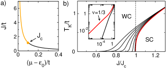
Figure 2: (color online) a) Kondo coupling vs. gate $\mu$ for $U/t=1$ and $V/t=0.3$. The dot illustrates a typical value for the critical coupling $J_{c}$. b) Kondo temperature $T_{K}/t$ vs. $J$ for $C_{3v}$ invariant orbitals. Red (light) curve: $\mu=0$; black: $\mu/D=$0.05, 0.1, 0.15, 0.2, $0.25$, and 0.3. The line $J\sim J_{c}$ sets the crossover scale between the Kondo weak coupling (WC) and strong coupling (SC) regimes. Inset: $T_{K}/t$ vs. $J/J_{c}-1$ near the QCP ($\mu=0$), in log scale. Red (light) line: type II orbitals ($\nu=1/3$); black: type I ($\nu=1$) (see text).

In Fig. 2b, we numerically calculate the scaling of the Kondo temperature in tight-binding. For type II orbitals, the $\nu=1/3$ exponent in the Kondo temperature, $T_{K}\propto|J-J_{c}|^{\nu}$, found in the linear cone approximation persists above room temperature, up to $T_{K}/t\sim 1$ (red curves). In the more standard ohmic case, for spins on top carbon sites (black curve of the inset), the scaling is linear ($\nu=1$) at the mean-field level.

Tracing the conduction electrons in the exchange Hamiltonian (6), the RKKY Hamiltonian of a spin lattice in graphene is $H_{RKKY}=-J^{2}\sum_{ij}\chi_{ij}^{x,y}\,\mathbf{S}_{i}\cdot\mathbf{S}_{j}\,,$ where $\chi_{ij}^{x,y}\equiv\chi^{x,y}(\mathbf{R}_{i}-\mathbf{R}_{j})$ is the spin susceptibility, with $i,j$ indexing the local spins, and $x,y=A,\,B,\,H,\,S_{A},\,S_{B}$ label the position of the magnetic adatoms in lattice. In momentum space,

$$\chi^{x,y}(\mathbf{q})=\sum_{\alpha\alpha^{\prime},\mathbf{p}}\mathcal{M}_{\alpha,\alpha^{\prime}\mathbf{p},\mathbf{q}}^{x,y}\frac{n[E_{\alpha^{\prime}}(\mathbf{p}+\mathbf{q})]-n[E_{\alpha}(\mathbf{p})]}{E_{\alpha^{\prime}}(\mathbf{p}+\mathbf{q})-E_{\alpha}(\mathbf{p})}\,,$$ (12)

where $\mathcal{M}_{\alpha,\alpha^{\prime},\mathbf{p},\mathbf{q}}^{xy}=\Theta_{\alpha\mathbf{p}}^{*x}\Theta_{\alpha\mathbf{p}}^{y}\Theta_{\alpha^{\prime}\mathbf{p}+\mathbf{q}}^{x}\Theta_{\alpha^{\prime}\mathbf{p}+\mathbf{q}}^{*y}$.

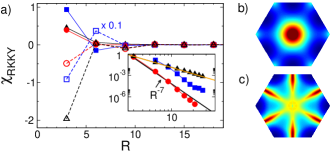
Figure 3: (color online) a) $\chi(R)$ vs distance $R$, along a zigzag direction (in lattice units), for $A$-sites (black triangles), $H$-sites (blue squares), and $S$ sites for spins on the same sublattice (red circles). Solid lines: $\mu=0$; dashed: $\mu=t$. Inset: $|\chi_{ij}|$ plot in a log scale. Orange (light) guide line: $1/R^{3}$; black: $1/R^{7}$. On the right: $\chi(\mathbf{q})$ for $A$ site spins, plotted in the graphene BZ at b) $\mu=0$ and c) $\mu=t$. Red (dark) regions represent $\chi(\mathbf{q})>0$ and blue (light) regions $\chi(\mathbf{q})<0$.

For spins on the same sublattice, $\mathcal{M}^{AA}\!=\!1/4$, whereas on opposite sublattices $\mathcal{M}^{AB}\!=\!\alpha\alpha^{\prime}\phi_{\mathbf{p}}\phi_{\mathbf{p}+\mathbf{q}}^{*}/(4|\phi_{\mathbf{p}}||\phi_{\mathbf{p}+\mathbf{q}}|)$, in agreement with Ref.Brey , in the Dirac cone limit. For an $H$-sitenote ,

$$\mathcal{M}^{HH}=|\Theta_{\alpha,\mathbf{p}}^{H}|^{2}|\Theta_{\alpha^{\prime},\mathbf{p}+\mathbf{q}}^{H}|^{2},$$ (13)

where $|\Theta_{\alpha,\mathbf{p}}^{H,\gamma}|^{2}=|\phi_{\mathbf{p}}|^{2}\left[1+(-1)^{\gamma}\alpha\mbox{Re}(\phi_{\mathbf{p}}^{3})/|\phi_{\mathbf{p}}|^{3}\right]$ for orbitals of type II; for $S$-sites, $\mathcal{M}^{S_{A}S_{A}}=|\phi_{\mathbf{p}}|^{2}|\phi_{\mathbf{p}+\mathbf{q}}|^{2}/4$ for spins on the same sublattice, and $\mathcal{M}^{S_{A}S_{B}}=\alpha\alpha^{\prime}\phi_{\mathbf{p}}^{3}\phi_{\mathbf{p}+\mathbf{q}}^{*\,3}/(4|\phi_{\mathbf{p}}||\phi_{\mathbf{p}+\mathbf{q}}|)$ for opposite ones.

In Fig. 3a, we show the spacial decay of the RKKY interaction on the lattice for type II orbitals on $A$, $H$ and $S_{A}$ site spins. At half filling, the RKKY interaction is always ferromagnetic for same sublattice spins, substitutional or not, and antiferro for spins on opposite sublatticesSaremi ; Brey . The $H$ case on the other hand, is ferromagnetic for nearest neighbor spins and antiferromagetic at longer distances (blue squares). In the $H$ and $S$ cases, the interaction is short ranged and decays with a fast power law $\sim 1/R^{7}$, in contrast to the known $1/R^{3}$ decay in the $A$ site caseVozmediano ; Cheianov ; Saremi ; Brey , as shown in the inset of Fig. 3. This fast decay is consistent with the case of carbon nanotubes, where the RKKY interaction decays with $1/R$ for top carbon sites and with $1/R^{5}$ for isotropic orbitals on $H$ sitesKirwan .

Fig. 3b and 3c display the magnetic peaks in the susceptibility in the $A$-site case for $\mu=0$, and $\mu=t$. For $\mu<t$, $\chi(\mathbf{q})$ has a strong ferromagnetic forward scattering peak around the center of the BZ ($q=0$), and six subdominant antiferromagnetic peaks at corners of the BZ. Exactly at $\mu=t$, a strong peak emerges at the $M$ point due to the nesting of the Van-Hove singularities (VHS) of the graphene band (see Fig. 3c), where the DOS diverges logarithmically. This peak reverses the ordering pattern of the RKKY interaction in comparison to the $\mu=0$ regime in all studied cases, as shown in the dashed lines of Fig. 3a. When $\mu$ is at the VHS, the interaction between spins on same (opposite) sublattices, substitutional or not, is always antiferromagnetic (ferro). In the same way, the RKKY interaction in the $H$ site case becomes antiferromagnetic for nearest neighbor sites and ferromagnetic at long distances.

In conclusion, we have derived the one-level exchange Hamiltonian for magnetic adatoms in graphene and shown the existence of two symmetry classes of magnetic orbitals that correspond to distinct classes of Kondo QCP. We also showed that the exchange coupling can be controlled across the quantum critical region with the application of a gate voltage.

We thank E. Fradkin, A. Balatsky, L. Brey and S. Lal for discussions. BU acknowledges partial support from the DOI grant DE-FG02-91ER45439 at University of Illinois. TGR acknowledges support of CNPq and FAPERJ. AHCN acknowledges DOE grant DE-FG02-08ER46512.

Erratum: Kondo Quantum Criticality of Magnetic Adatoms in Graphene
[Phys. Rev. Lett. 106, 016801 (2011)]

Bruno Uchoa, T. G. Rappoport, and A. H. Castro Neto

In Ref.uchoa_E we have predicted the existence of two different classes of quantum critical points for the Kondo problem in graphene, which was shown to correspond effectively to the problem of a localized spin $1/2$ coupled to a fermionic bath with electronic density of states $\rho(\omega)\propto|\omega|^{\bar{r}}$, with $\bar{r}=1$ or $3$. Here we point out that the mean field exponent $\nu=1/3$ derived within the slave boson approach for the class of orbitals of type II $(\bar{r}=3$) is incorrect.

Above the upper critical scaling dimension of the Anderson model ($\bar{r}>1$), the intermediate coupling fixed point is non-interacting and describes the level crossing between singlet and doublet states with the trivial exponent $\nu=1$Vojta_E . Albeit fluctuations do not play a role in the critical behavior for $\bar{r}>1$, the critical theory is not of the Ginzburg-Landau type and the validity of the mean-field slave boson equation of state (9) breaks down in the $\bar{r}=3$ class, invalidating Eq. (10), (11), and the inset of Fig. 2b for the case of type II orbitals.

All the other results of the paper remain valid, including the spin exchange Hamiltonian in Eq. (6) and the prediction of a fast power law for the spatial decay of the RKKY interaction for type II orbitals ($\sim 1/R^{7}$).

We note that since hyperscaling is not obeyed for $\bar{r}>1$, the scaling prediction for the Kondo temperature with the chemical potential, $\mu$, in the quantum critical region, $T_{K}\propto|\mu|$, can be violatedVojta2_E . In the situation where the scaling prediction fails, the criticality in the $\bar{r}=1$ and $\bar{r}=3$ classes can be in principle distinguished. That will be verified with NRG methods elsewhere.

We acknowledge M. Vojta for many helpful discussions.

References

(1)A. H. Castro Neto et. al.,Rev.
Mod. Phys.81, 109 (2009).
(2)L. S. Mattos et al. (to be published).
(3)J.-H. Chen et al., arXiv:1004.3373 (2010).
(4) D. Withoff and E. Fradkin, Phys. Rev. Lett. 64,
1835 (1990).
(5)G.-M. Zhang et al., Phys. Rev. Lett. 86,
704 (2001); B. Dora et al., Phys. Rev. B 76, 115435
(2007); P. S. Cornaglia et. al., Phys. Rev. Lett. 102,
046801 (2009); C. R. Cassanello, and E. Fradkin, Phys. Rev. B 53,
15079 (1996); Phys. Rev. B 56, 11246 (1997).
(6)M. Hentschel et al., Phys. Rev. B 76,
115407 (2007).
(7)K. Sengupta et. al., Phys. Rev. B 77, 045417 (2008).
(8)T. O. Wehling et al., Phys. Rev. B 81,
115427 (2010).
(9)B. Uchoa et al., Phys. Rev. Lett. 103,
206804 (2009).
(10)H.-B. Zhuang et. al., Europhys. Lett. 86,
58004 (2009).
(11)K. Saha et al., Phys. Rev. B 81,
165446 (2010).
(12)T. O. Wehling et. al., Phys. Rev. B 81, 115427
(2010).
(13) P. W. Anderson, Phys. Rev. 124, 41
(1961).
(14)B. Uchoa et. al., Phys. Rev. Lett. 101,
026805 (2008).
(15) A. V. Krasheninnikov et al., Phys. Rev. Lett.
102, 126807 (2009).
(16)A. J. Leggett et al., Rev. Mod. Phys. 59,
1 (1987).
(17)J. R. Schrieffer et al., Phys. Rev. 149,
491 (1966).
(18) The condition
is also required.
(19) In this limit, is regularized by midgap states
induced by the scattering potential of the impurity. See Ref. Hentschel .
(20)M. Pustilnik et al., Phy. Rev. Lett. 87,
216601 (2001).
(21)D. M. Newns and N. Reed, Adv. Phys., 36,
799 (1987).
(22)M. Vojta, and L. Fritz, Phys. Rev. B 70,
094502 (2004).
(23) M. Vojta et al., arXiv:1002.2215 (2010).
(24)S. Saremi, Phys. Rev. B 76, 184430 (2007).
(25)L. Brey, et al., Phys. Rev. Lett. 99,
116802 (2007).
(26)The RKKY interaction for -sites is not described
by the charge polarization, as suggested in Ref. Brey .
(27)M. A. H. Vozmediano, et al. Phys. Rev. B 72,
155121 (2005).
(28)V. Cheianov et. al., Phys. Rev. Lett. 97,
226801 (2006).
(29)D. F. Kirwan, et al., Phys. Rev. B 77,
085432 (2008)