Dynamical studies of macroscopic superposition states: Phase engineering of controlled entangled number states of Bose-Einstein condensates in multiple wells

Abstract

We provide a scheme for the generation of entangled number states of Bose-Einstein condensates in multiple wells with cyclic pairwise connectivity. The condensate ground state in a multiple well trap can self-evolve, when phase engineered with specific initial phase differences between the neighboring wells, to a macroscopic superposition state with controllable entanglement – to multiple well generalization of double well NOON states. We demonstrate through numerical simulations the creation of entangled states in three and four wells and then explore the creation of “larger” entangled states where there are either a larger number of particles in each well or a larger number of wells. The type of entanglement produced as the particle numbers, or interaction strength, increases changes in a novel and initially unexpected manner.

I Introduction

Entanglement, a nonclassical correlation between two or more physical systems, lies at the heart of the profound difference between quantum mechanics and a local classical description of the world einstein1935 . Apart from their discussions in the philosophical and foundational aspects of quantum mechanics bell1987 , entangled states in recent years have become an essential resource for the emerging field of quantum information processing horodecki2009 . Entangled and squeezed states hold promise in studies related to quantum measurement, Heisenberg limited atom interferometry and precision measurements huelga1997 ; pezze09 , and quantum computing and quantum communication. Since multi-particle entangled states can be more useful than the two-particle/two-photon states, there have been steady attempts toward creating such states monroe2002 . Such states have been created with several systems – with five photons zhao2004 , eight atoms in an ion trap haffner2005 , ten nuclear spins in a molecule jones2009 , and also with cold atoms in an optical lattice mandel2003 ; oberthaler2008 . There have been several proposals to create superposition states with a large number of particles such as using a tiny mirror marshall03 and microorganisms such as viruses cirac10a .

While the consequence of entanglement for an Einstein-Podolsky-Rosen (EPR) pair is quantified in Bell’s inequality bell1965 , a more striking conflict between quantum mechanics and local realism is exhibited by three maximally entangled spins also known as the Greenberger-Horne-Zeilinger (GHZ) states greenberger1990 . GHZ state of $N$ spins has the form

$$|\Psi\rangle=\frac{1}{\sqrt{2}}\left(|{N},0\rangle+|0,{N}\rangle\right)$$ (1)

This state can also be written in the notation $|00...0\rangle+|11...1\rangle$ where $|0\rangle$ and $|1\rangle$ are the basis states. The superposition of two macroscopically distinct states, rather than simply the internal degrees of freedom, each occupied by all $N$ particles, has been discussed by Schrödinger in the famous cat parable sch1935 ; partial realization of such Schrödinger’s cat states has been obtained with Josephson junction loops friedman00 ; lloyd00 . That macroscopic superposition states are highly entangled has been discussed in Ref. morimae10 .

The analog for the GHZ state for ${N}$ particles in two wells is denoted like Eq. 1, $\frac{1}{\sqrt{2}}(|{N},0\rangle$ + $|0,{N}\rangle)$, and is colloquially referred to as “NOON” states. A generalization of this two state model to multi dimensions has been discussed in Ref. cerf2002 . In this paper, we discuss the generation of macroscopic entangled number states of a multiwell Bose-Einstein condensates (BEC) of the approximate form

$$|\Psi\rangle_{\{{N},M\}^{max}} = \frac{1}{\sqrt{M}}(|{N},0,0,\ldots,0\rangle+|0,{N},0,\ldots,0\rangle$$ (2)

$$+\ldots+|0,0,\ldots,{N}\rangle$$

This is the multiwell generalization of the double well NOON states where a macroscopic number of particles are simultaneously in $M$ different locations, with $M>2$. BEC in optical lattices review has been a promising research area with many new observations such as the superfluid to Mott insulator transition greiner2002 and number-squeezed states orzel2001 . Superfluid and Mott insulator states are the ground states of bosons in an optical lattice, whereas the multi-positional Schrodinger cat state of type Eq. 2 is the highest lying excited state. Due to the coherence properties and versatility of cold atom systems, it may be an ideal system to create such entangled states.

We show that states approximating the extreme entangled states of Eq. 2 may be generated in a controlled fashion by time evolution of appropriately phase imprinted ground states of a multiwell BEC with periodic boundary conditions for $M=3,4$, and $8$. The physical mechanism for creating such states can be understood from the phase space picture of a double well BEC mahmud2005 ; mahmudThesis where it was shown that the ground state wave packet displaced in phase and put on a hyperbolic fixed point of its underlying semiclassical phase space dynamically bifurcates to a macroscopic superposition state, a highly entangled state. Similarly, for a multi-well BEC, phase imprinting the ground state moves it to an unstable equilibrium, and subsequent dynamics creates entangled states. We show that the choice of initial barrier heights, which determine the extent of ground state number squeezing, and the rate of barrier ramping can be used to control the entanglement of the final states.

Based on results obtained for two, three, and four well configurations, we conjecture a generalized formula, for $M$ wells, for the phase offset between neighboring wells appropriate for the generation of number entangled states. Finally, we extend our analysis to larger systems where there are a larger number of particles in each well or a larger number of wells. In these cases, we find surprising results indicating the formation of a new type of number entangled state in four wells. We study the impact of increasing the number of particles or the interaction strength on the resultant entangled state.

The paper is organized as follows. In Sec II, we introduce our model and discuss the numerical methods. In Sec III, we review previously published mahmud2005 results for the generation of NOON like entangled states in a double well. This is done in order to motivate and generalize the double well results to multiple wells. In Sec IV, we present our study of three and four wells showing the phase engineering method for creating entangled states. We focus on small number of particles, mainly showing that the method works for multiple wells, and that we can control the final state by controlling the initial barrier height and barrier ramps. In Sec V, we study this for larger number of particles in four and eight wells, and find that a new type of entangled number state is also created in the process. Finally, we summarize our results in conclusion in Sec VI.

II Methods

Figure 1: Shown are multi-well configurations for three, four, and eight wells with periodic boundary conditions in a one dimensional circular array.

The physical configuration we study assumes multiple wells connected in a circular array, which has been realized experimentally by amico2005 , and is illustrated in Fig. 1.

We approximate the physics of a BEC in a multiwell potential by the Bose-Hubbard (BH) model fisher1989 ; jaksch1998 . Thus

$$\hat{H} = -J\sum_{i}(a_{i}^{\dagger}a_{i+1}+a_{i+1}^{\dagger}a_{i})+\sum_{i}\epsilon_{i}\hat{n_{i}}$$ (3)

$$+\frac{1}{2}U\sum_{i}\hat{n_{i}}(\hat{n_{i}}-1)$$

where $\hat{n_{i}}=a_{i}^{\dagger}a_{i}$ is the number operator, $J$ is the nearest neighbor tunneling term, $U$ is the on-site energy, and $\epsilon_{i}$ is the energy offset of the $i$th lattice. To simplify a theoretical study, we make a one parameter approximation of the tunneling and interaction strength: $U/J=1/e^{-\alpha(t)}$; and for the symmetric wells explored here, $\epsilon_{i}=0$. Because of the tunability in optical lattices, $U$ and $J$ can be changed in time with varying lattice depth, and we take $\alpha(t)$ as a function of time $t$. $\alpha(t)$ is a dimensionless parameter that can be mapped onto the barrier height. This parametrization allows a simple study of continuous change of barrier height through the variation of a single parameter $\alpha(t)$. For example, for a lattice made of red detuned laser with $\lambda=985$ nm and for ²³Na, a barrier height $15E_{R}$ gives $U=0.15E_{R}$ and $J=0.07E_{R}$ jaksch1998 where $E_{R}=\frac{\hbar^{2}k^{2}}{2m}$ is the recoil energy from absorption of a photon; these experimental parameters then correspond to $\alpha=2.14$.

Our numerical studies focus on three size regimes: I) a small number of particles in a small number of wells, II) a large number of particles in small number of wells, similar to the experiments of orzel2001 , and III) a small number of particles in a larger number of wells, such as the experiments of greiner2002 . For ${N}$ identical bosons in $M$ wells the number of Hilbert space dimension is $D=\frac{({N}+M-1)!}{{N}!(M-1)!}$. The latter two cases result in large $D$ and necessitate the use of parallel processing techniques. The largest systems we have investigated at the time of writing is 512 particles in four wells with 202 million nonzero entries, $D$=22,632,705 and 24 particles in eight wells, $D$=2,629,575 with 3.5 million nonzero entries. Details of our parallel implementation of the Bose Hubbard model can be found in leung2007 .

The main equation we solve is the time dependent Schrödinger equation (TDSE):

$$\sum_{k}[H]_{jk}c_{k}(t)=i\hbar\frac{dc_{j}(t)}{dt}$$ (4)

where $H$ is the discretized BH Hamiltonian in the Fock state basis $|m\rangle$. The solution of the time dependent Schrödinger equation in the full Fock space is then of the form

$$|\Psi(t)\rangle=\sum_{m=0}^{D-1}{c_{m}(t)|m\rangle}$$ (5)

III Entangled number states of the BEC in two wells

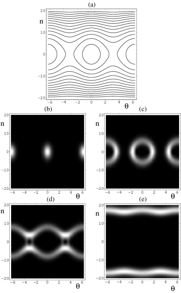
Figure 2: Comparison of the classical nonrigid physical pendulum phase space with quantum phase space shown with the Husimi probability distributions for double well eigenstates. Shown are (a) classical energy contour. Husimi projections for (b) ground state which is minimum uncertainty wavepacket centered at the origin, (c) 6th state, (d) 12th state, and (e) 35th state which is analogous to a superposition of classical pendulum rotor motions in two opposite directions. The analogy between the double well BEC and physical pendulum points to a way to the creation of macroscopic superposition states by displacing the ground state to the unstable equilibrium points in the classical phase space.

In order to generalize the creation of entangled states in multiple wells, we briefly review here the physical principles behind creating such states in a double well which was described in Ref. mahmud2005 ; mahmudThesis . The physics of creating such states in a double well as well as its extension to multiple wells as presented here can be understood in terms of the underlying classical phase space dynamics.

The most general state vector in a double well is a superposition of all the number states

$$|\Psi\rangle=\sum_{n_{L}=0}^{N}c^{(i)}_{n_{L}}|n_{L},N-n_{L}\rangle$$ (6)

where $n_{L}$ is the number of particles in the left well, and $N$ the total number of particles. Finding the eigenvalues and eigenvectors of the Bose-Hubbard hamiltonian for two wells can be easily accomplished by diagonalizing a $(N+1)\times(N+1)$ tridiagonal matrix, getting the coefficients $c^{(i)}_{n_{L}}$.

After we implement the cat state generation method, states of the following form can be generated,

$$|\Psi\rangle=\frac{1}{\sqrt{2}}\left(|N-n_{L},n_{L}\rangle+|n_{L},N-n_{L}\rangle\right)$$ (7)

When $n_{L}=0$ or $N$, it becomes an extreme superposition state

$$|\Psi_{extreme}\rangle=\frac{1}{\sqrt{2}}\left(|N,0\rangle+|0,N\rangle\right)$$ (8)

where all the particles are simultaneously in the left and right wells. Here the cat states are positional NOON states where $N$ particles occupy spatially separated modes in two wells. There can also be NOON states of other kinds such as with $N$ particles occupying the two quasi-momentum modes of counter-propagating superfluid flow states in a rotating ring lattice that have been proposed in Ref. dunningham2006 ; nunnenkamp08 .

Anderson manybody1964 showed that the Hamiltonian for a system of two quantum fluids connected by a tunneling junction can be described as a physical pendulum. For BEC in a lattice, in the semiclassical limit valid for large $N$, the operators $\hat{a_{i}}$ in Eq. 3 can be approximated by the c-numbers $\sqrt{n_{i}}e^{i\theta_{i}}$, where $n_{i}$ and $\theta_{i}$ are the number and phase of particles in the $i$th well. For a two site Bose-Hubbard model, the Hamiltonian then turns into a classical Hamiltonian of a nonrigid physical pendulum with the number and phase differences ($n=(n_{L}-n_{R})/2$,$\theta=\theta_{L}-\theta_{R}$) between the wells as conjugate variables. The dynamics of double well BEC is then described by a classical pendulum model that has been studied in detail in Ref. smerzi1997 and experimentally verified in  albiez05 . Fig. 2(a) shows the classical energy contour showing the classical phase space structure. This system has two fixed points – (0,0) and (0,$\pi$). The (0,0) is a stable equilibrium, while the (0,$\pi$) is stable in the $\pi$-state regime ($UN/J<1$) and unstable otherwise ($UN/J>1$). Two types of pendulum motions – oscillations and rotor motions appear in the phase space, below and above the separatrix. Question can be raised on how much of the classical phase space is actually contained in a full quantum analysis. This was answered in Ref. mahmud2005 showing quantum-classical correspondence between the classical pendulum and double well BEC.

Husimi probability distribution mahmud2005 ; husimi40 can be used to project, in a squeezed coherent state representation, the classical phase space properties from quantum wavefunctions. In $(n,\theta)$ representation, Husimi function is defined as

$$P_{j}(n,\theta)=|\langle\theta+in|\Psi_{j}\rangle|^{2}$$ (9)

where

$$\langle\theta+in|\Psi_{j}\rangle=\frac{1}{(\pi\kappa)^{1/4}}\sum_{n^{\prime}=-N/2}^{N/2}c^{j}_{n^{\prime}}\exp[i\theta n^{\prime}-\frac{(n^{\prime}-n)^{2}}{2\kappa}]$$ (10)

Here $n^{\prime}=\frac{n_{L}-n_{R}}{2}$, rather than being the simpler left particle counter, and $c_{n^{\prime}}$ is the corresponding Fock-state coefficient. The ‘coarse-graining’ parameter $\kappa$ determines the relative resolution in phase space in the conjugate variables number and phase.

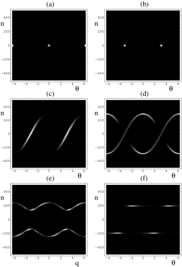
Figure 3: A visual depiction of the underlying physical principles for the generation of entangled states in a double well. Quantum phase space pictures of Husimi projections are plotted here - (a) the ground state at t=0, (b) $\pi$-phase imprinted ground state at the hyperbolic fixed point, (c) at t=0.012 ms the wavepacket is bifurcating along the separatrix, (d) at t=0.019 ms it continues to move along the separatrix, (e) with simultaneous ramping of the barrier the wavepacket splits completely at t=0.49 ms, and (f) at t=2.84 ms a sharply peaked entangled state is obtained which is a macroscopic superposition of particles simultaneously in both wells.

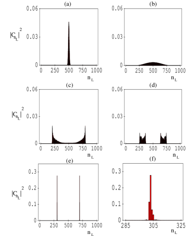
Figure 4: Shown is the evolution to a cat state in Fock space at the same time instants as in the previous figure: (a) the phase imprinted ground state at t=0, (b) at t=0.012 ms the Gaussian distribution broadens, (c) at t=0.019 ms it bifurcates, (d) at t=0.49 ms it splits completely, (e) at t=2.84 ms a highly entangled state is formed; (f) is a magnified version of (e) showing the nonvanishing Fock state coefficients.

Figs. 2(b)-(e) show representative Husimi projections for 40 particles for the ground state, 6th , 12th and 35th states respectively. The ground state is a wave packet centered on (0,0) in the classical phase space, with a finite width in number and phase differences. The higher lying states in (c) is a harmonic oscillator like state, (d) is a state which lies on the separatrix and (e) is a cat state, which in classical sense, is a superposition of clockwise and counter-clockwise pendulum rotor states. After understanding this quantum-classical correspondence, we can argue that a ground state wave packet displaced in phase by $\pi$ and put onto the unstable fixed point (0,$\pi$) would bifurcate along the separatrix and create a superposition of two pendulum rotor states, if allowed to time evolve. The $\pi$ displacement of the ground state can be accomplished by phase imprinting one of the wells by an amount $\pi$ which in experiments could be done by a phase engineering technique that has been demonstrated in experiments investigating solitons in the BEC denschlag2000 .

For a concrete example of our method, we show results of a numerical simulation in Figs. 3 and 4. Fig. 3 demonstrates the underlying physical principles quite visually in quantum phase space using Husimi projections. First in panel (a) we have a ground state that is at the center of phase space, then in (b) we displace this by $\pi$ in the horizontal direction so that it is on an unstable equilibrium. Since it is no longer an eigenstate, it will time evolve spontaneously, and in this case the trajectories in phase space follow along the separatrix and symmetrically spits in two directions as in (c) at t=0.012 ms. In this process the phase space points reach the top and bottom of the separatrix as in (d) at t=0.019 ms. If we simultaneously increase the barrier height during this time evolution, we can completely split the top and bottom as shown in (e) at t=0.49 ms, finally giving rise to a desired cat state in (f) at t=2.84 ms. The times for this example of double well as well as three wells in next section are given for a ⁸⁷Rb condensate, $\lambda=840$ nm, $a_{sc}=5.8$ nm, $J=0.04E_{R}e^{-\alpha}$ where $E_{R}=\frac{\hbar^{2}k^{2}}{2m}$ is the recoil energy from absorption of a photon, and $\alpha$ is a dimensionless parameter that can be mapped onto the inverse tunneling rate, and taking $U=0.04E_{R}$ as approximately constant for calculation purposes. Here $\alpha$ varies as $\alpha=3+2t$. The evolution to an entangled state is shown in Fock space coefficients in Fig. 4 – the process of the formation of a superposition state can also be understood from this. For a two-component spinor Bose gas, Ref. micheli03 shows the generation of entangled state, where there is no need for initial phase imprint. We demonstrate here the generation of number entangled cat states of the NOON type; we do not discuss generation of phase cat states piazza08 that are superpositions of many coherent phase states. Much of the intuition for later sections is derived from an in depth study of the double well as briefly described here and presented in detail in mahmud2005 .

IV Entangled number states in three and four wells with small particle number

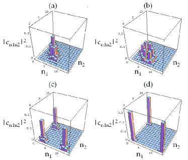
Figure 5: (color online). Fock state coefficients for 12 particles in three wells: (a) the ground state, (b) 10th, (c) 76th and (d) 91st, the highest state. The ground state has a Gaussian shape, while higher lying states are entangled number states. $n_{1}$ and $n_{2}$ are the Fock state indices and the vertical axis shows probabilities. Points beyond the cross-diagonal are unphysical.

In order to gain insight into the multiwell Bose-Hubbard model, we first analyze the quantum mechanical properties of the simplest multiwell potential, $M=3$, assuming three symmetric wells in a circular array circularandlineararray .

The state vector for three wells is a superposition of all the number states

$$|\Psi_{i}\rangle=\sum_{n_{1},n_{2}=0}^{N}c_{n_{1},n_{2}}^{(i)}(t)|n_{1},n_{2},n_{3}\rangle$$ (11)

Here $n_{1}$, $n_{2}$, and $n_{3}={N}-n_{1}-n_{2}$ are the number of particles in each of the three wells. Fig. 5 shows the Fock space probabilities, $\left|c_{n_{1},n_{2}}^{(i)}\right|^{2}$, for representative stationary states for $N=12$ and $\alpha=0$ ($U/J=1$). $n_{1}$ and $n_{2}$ are the Fock state indices and the vertical axis shows probabilities. The ground state in Fig. 5(a) is a broad Gaussian while the higher lying states, Figs. 5(c)-(d), are number entangled states of increasing extremity corresponding to increasing numbers of particles simultaneously in all three wells, the highest of which in panel (d) approximates an extreme superposition state of the form $|N,0,0\rangle+|0,N,0\rangle+|0,0,N\rangle$. Note that there are still some nonvanishing Fock space components. As $U/J$ increases the highest lying state approaches the extreme state of Eq 2. The number of non vanishing Fock state coefficients determines sharpness, and thus (d) is sharper than (c).

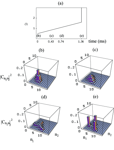
Figure 6: (color online). Evolution to an entangled Fock space state for three wells: (a) barrier ramp showing the location of the following time evolved states: (b) initial state, (c) at 0.43 ms the Gaussian distribution broadens, (d) at 0.74 ms the distribution is ‘splitting’, (e) A three-peaked state is formed at 1.36 ms; a macroscopic superposition of definite number of particles simultaneously in all three wells. A comparison with the double well Fock state evolution in Fig. 4 shows that the physical mechanism for generating entangled states is the same in a double well and multiple wells.

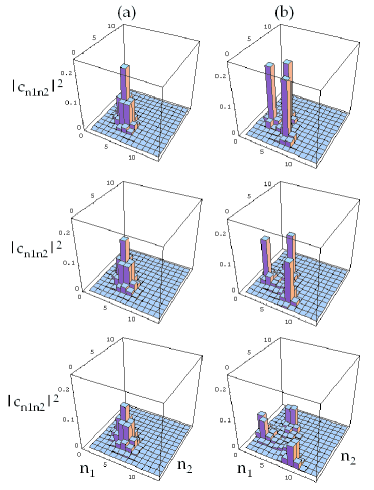
Figure 7: (color online). Entangled states evolved from ground states with different initial squeezing. Row (1) shows the states with $\alpha=1.0+t$: (a) initial ground state and (b) final state. Row (2) is for $\alpha=0.5+t$ and (3) is for $\alpha=t$. Column (b) gives the states at t=1.85 ms, t=1.36 ms, and t=0.99 ms respectively. The initial squeezing of the ground state thus determines the extremity of the resulting entangled states.

It is unlikely that such maximally entangled states can be generated via a sequence of single particle excitations. They may however, be dynamically generated via phase engineering from the appropriate ground state, as elucidated in previous section for the double well. Writing phases on part of a condensate is experimentally feasible via interaction with a far off-resonance laser denschlag2000 , and is assumed to be sudden with respect to the dynamics of the condensate. Mathematically, this corresponds to multiplying the coefficients in an expansion of the type of Eq. 5 by $e^{in_{i}\theta_{i}}$, where $|n_{1},n_{2},...n_{i},...\rangle$ is the corresponding Fock state, and $\theta_{i}$ is the phase for particles in the $i$th well.

Entangled state generation, obtained via integration of the linear time-dependent Schrödinger equation, is shown in Fig. 6, following phase imprinting of an initial phase difference of $\frac{2\pi}{3}$ between the neighboring wells, and a simultaneous linear ramping of the barrier as $\alpha=0.5+t$, as shown in Fig. 6(a) (t here is dimensionless). Panels 6(b) shows the initial ground state; 6(c) at time 0.43 ms, the distribution broadens; 6(d) at 0.74 ms, in the process of splitting the state towards the three corners; and 6(e) at 1.36 ms a sharp, although not extreme, entangled number state with its signature of three major non vanishing expansion coefficients.

When an appropriately entangled state is reached the barrier is suddenly raised to halt further evolution in n-space. For the parameter values used here, a simple time evolution without any change of barrier also produces an entangled state, however barrier ramping is used here to sharpen the resulting state, and completely split Fock state coefficients into three parts. Control of the extremity of the states can be achieved by choice of the initial barrier height controlling the initial squeezing of the ground state. This is demonstrated in Fig. 7, where different initial squeezing have been used for rows (1), (2) and (3). The columns show: (a) the ground state, and (b) the final state at the end of the barrier ramping. It is important to be able to tune to less extreme entangled states, as such states are more robust to loss and decoherence mahmud2005 ; mahmudThesis . In our study here, we show the proof of principles that cat states can be produced and controlled. To be able to get extreme superpositions, analysis can be made with optimal control theory on the correct parameters and ramping to be used. Phase imprinting with a phase difference of $\frac{4\pi}{3}$ produces an equivalent state, with different phase space dynamics.

What is so special about phase imprinting $\frac{2\pi}{3}$? Similar to the simple double well, the triple well, $M=3$, can be thought of as two coupled pendulums franzosi2003 with complicated dynamics – quantum and semiclassical aspects of three well BEC have been elucidated in Ref. mossman06 ; trimborn09 ; viscondi10 . Here the semiclassical conjugate variables are $\Delta n_{12}=n_{1}-n_{2}$, $\Delta n_{23}=n_{2}-n_{3}$, $\Delta\theta_{12}=\theta_{1}-\theta_{2}$ and $\Delta\theta_{23}=\theta_{2}-\theta_{3}$. The unstable fixed points in these conjugate variables are (0,0,$\frac{2k\pi}{3}$,$\frac{2k\pi}{3}$), $k=1,2$. So, a phase imprint of $\frac{2\pi}{3}$ or $\frac{4\pi}{3}$ puts the ground state wavepacket on the unstable equilibrium, and subsequent dynamics gives rise to these states.

Figure 8: (color online). Four well stationary and time evolved states: (a) ground state, (b) an entangled state evolved from the ground state following a $\pi$ relative phase shift. The three dimensions show the Fock state indices $n_{1}$, $n_{2}$ and $n_{3}$, probabilities are shown in the color intensity scale. For graphical clarity, only the points higher than $40\%$ of the highest probability are shown, with the highest probabilities normalized to 1.

Figure 9: Initial phase configurations that generate number entangled states. These phase differences are motivated by the fixed point of the underlying semiclassical phase space – bifurcation characteristics of the unstable equilibrium generating the macroscopic superpositions. Shown here are examples for a double well (a), triple well (b and c), and four wells (d, e and f). There are $M-1$ different possibilities for $M$ wells. The known case of $\pi$ phase differences for an even number of wells is seen to be a special case.

One important aspect of our method is the controllability of the final state which works for multiple wells as illustrated in Fig. 7. It works in three ways – I) A simultaneous ramping of the barrier with the natural dynamics at the unstable fixed point has been empirically found to be useful in directing the desired evolution of the wavepacket. II) Initial barrier height, that is the initial squeezing, helps shape the initial wave packet stretching it into different regions of accessible phase space; and, III) the initial barrier height sets the (negative) curvature of the potential at the hyperbolic fixed point, controlling the rate of splitting of the wave packet.

We found that all the features of the double well entanglement generation apply to the three well case, and thus, many of the insights from the two and three well dynamics can be extended to arbitrary number of wells in a circular array. Next, we explore it for four wells. For four wells, the values of phase imprints that take the ground state to fixed points are $\frac{\pi}{2}$, $\pi$ and $\frac{3\pi}{2}$. Fig. 8(a) shows a typical ground state in four wells that is an approximate Gaussian. After a phase imprint of $\pi$ between neighboring wells, the ground state can be evolved into an extreme entangled number state as shown in Fig. 8(b) for $N=16$, $U=0.01$ $E_{R}$, $J=0.04$ $E_{R}$ $e^{-\alpha}$, with $\alpha=0.175$, and assuming the case of ⁸⁷Rb in the previous example. Phase difference of $\pi$ between neighboring wells is equivalent to writing alternating $\pi$ phases on the lattice. The other fixed point dynamics of $\frac{\pi}{2}$ and $\frac{3\pi}{2}$ also lead to symmetric states but do not lead to the highly entangled states of the kind we discuss in this article.

In Ref. polkovnikov2002 , a truncated Wigner approximation was used to study an alternating $\pi$ phase difference dynamics for even number of wells. In comparing our four well results to theirs, we have done an exact time evolution study, and find that the $\pi$ configuration in an even number of wells that they have identified is just a special case of many phase imprint dynamics that could generate interesting correlated states in multiple wells. Their changes in system parameters is to drive the system from stability to a regime of instability. On the other hand, we take our system to be in the unstable regime and demonstrate the controllability of entangled states with barrier manipulation; potentially useful for experimental detection.

For the two, three, and four wells, we find $M-1$ distinct phase differences between the neighboring wells for the multi-well fixed points franzosi2003 . These are given by a general formula $\frac{2\pi j}{M}$ where $j=1,2,....M-1$, with $M$ being the number of wells, which gives a $\pi$ phase difference for the $M=2$ double well, a $\frac{2\pi}{3}$ and $\frac{4\pi}{3}$ phase difference for the $M=3$ triple well, and a $\frac{\pi}{2}$, $\pi$, and $\frac{3\pi}{2}$ phase difference for the $M=4$ quadruple well configuration – we investigated the dynamics generated by all of these phase difference imprints. Note that the total change in phase in the circular loop is a multiple of $2\pi$, a vortex like condition. We thus propose a general formula for $M$ wells,

$$\Delta\theta=\frac{2\pi j}{M}\text{,}$$ (12)

for the constant phase offset between neighboring wells leading to the dynamical generation of entangled states. Here $j=1,2,..,M-1$, and Eq. (12), being valid for any number of wells, even or odd, provides a substantial generalization of the $\pi$ phase offset mentioned in Ref. polkovnikov2002 , which is valid only for the special cases of an even number of wells and for $j=M/2$. Fig. 9 shows the phase configurations of Eq. (12). The multiplicity of Eq. (12) is prominent for large number of wells, e.g. for 12 wells, there are 11 phase offset possibilities. Symmetries may prevent all the imprinting offsets of Eq. 12 from generating independent dynamics.

Although detailed work on four and eight wells was done more recently and is being presented here as a coherent whole for multiple wells, the work on three well was done much earlier as documented in Ref. mahmudThesis ; mahmud04 . Many studies of quantum, semiclassical and entanglement aspects of three coupled BECs have appeared since then, that continue to explore the rich yet simpler lattice physics of the system of three well BEC.

V Large entangled number states in multiple wells

In this section we investigate the creation of large entangled number states where there are a large number of particles in each well and/or a large number of wells. Following the techniques described above and in leung2007 , we explored the creation of entangled number states in four and eight wells with periodic boundary conditions. We present results from our simulations of entangled number states in four wells in the Section V A, eight wells in V B, and in V C we analyze the types of entangled states generated and describe a new type of entangled number state.

In systems with wells $M>4$, visualization of multi-dimensional entangled states becomes more difficult. To facilitate the visualization we introduce the joint probability function

$$P(n_{\beta},n_{\gamma},t)=\frac{1}{M}\sum_{n_{i}=0,\forall i\neq\beta,\gamma}^{N}|c_{n_{1},n_{2},\ldots,n_{i},\ldots,n_{M}}(t)|^{2}$$ (13)

where the sum over $n_{i}$ does not include $n_{\beta}$ or $n_{\gamma}$, as they are held fixed and particle conservation requires a fixed total number of particles. $P(n_{\beta},n_{\gamma},t)$ shows the probability of finding $n_{\beta}$ particles in $\beta$th well simultaneously with finding $n_{\gamma}$ particles in the $\gamma$th well.

V.1 Large entangled number states in four wells

Figure 10: (color online). Ground and entangled number state for 128 particles in four wells: (a) Ground state and (b) entangled number state at $t=2.40$ ms for 128 particles in four wells, $U=0.01E_{R}$, $J=0.04e^{-\alpha}E_{R}$ with $\alpha=0.175$. The time shown in (b) represents the earliest time when maximum probability occurs for an entangled number state. Shown is the joint probability function $P(n_{1},n_{2})$ versus the number of particles in wells 1 and 2 on the $x$ and $y$ axes, respectively.

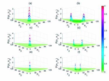
Figure 11: (color online). Varying the tunneling parameter, $J$, for four wells: (a) Ground state and (b) entangled number state for 128 particles in four wells with $U=0.01E_{R}$ and $J=0.04e^{-\alpha}E_{R}$ with $\alpha=0.175$ and $t=2.40$ ms, $\alpha=1.175$ and $t=3.65$ ms, and $\alpha=2.175$ and $t=5.70$ ms in rows 1, 2, and 3. This shows that initial squeezing can be used to control the final entanglement as have been shown for three wells in Fig. 7 and double wells in Ref. mahmud2005

The results of our investigation of the creation of entangled number states in four wells with a large number of particles in each well are provided below. The regime we explore in four wells is similar to the Kasevich orzel2001 experiments and we report results using experimental parameters relevant to their work for a condensate made of ${}^{87}Rb$ with $\lambda=840$ nm and $a_{sc}=5.8$ nm. We assume an intial phase offset of $\pi$ between the wells. Fig. 10 shows the joint probability function for (a) the ground state at $t=0$ and (b) entangled number state at time $t=2.40$ ms for 128 particles in four wells. In this figure and all following the time depicted represents the earliest time when maximum probability for an entangled state occurs. The ground state has a Gaussian distribution centered around the state where the particles are equally distributed between the wells. The joint probability function for the entangled number state has two peaks one where there are 57 particles in the $\beta=1$ well and 7 particles in the $\gamma=2$ well and another peak of equal probability where there are 7 particles in the $\beta=1$ well and 57 particles in the $\gamma=2$ well. Besides this highest probability state, there are other non-vanishing coefficients that are smaller and distributed around this peak.

Fig. 11 shows the effect of varying $J$, the tunneling parameter. Column (a) shows the joint probability function for the ground state at $t=0$ and column (b) shows an entangled number state at $t=2.40$, $3.65$, and $5.70$ ms in rows 1, 2, and 3, respectively. The tunneling parameter is set to $J=0.04e^{-\alpha}E_{R}$ with $\alpha=0.175$, $\alpha=1.175$, and $\alpha=2.175$ for rows 1, 2, and 3 respectively. Increasing $\alpha$ corresponds to decreasing tunnelling and correlates with increased time to evolve into the entangled number state. Increased $\alpha$ also means starting with a state with larger number squeezing, and thus we see in panels (a), (b) and (c) that the extremity of the final cat state is determined by initial squeezing. This same behavior was shown with double well mahmud2005 , and with three wells in the previous section, and thus we show that it is a general characteristic of multi-well cat states. We should emphasize the finding that to obtain a more extreme cat state, the initial barriers have to be low.

Fig. 12 illustrates the effect of varying the number of particles. Column (a) shows the ground state at $t=0$ and column (b) shows the entangled number state for 256 particles at $t=1.74$ ms, 384 particles at $t=1.47$ ms, and 512 particles at $t=1.30$ ms. Increasing the particle number raises the strength of the interaction term in the BH Hamiltonian and results in decreased tunneling, explaining the increased squeezing of the ground and entangled number states with increased particle number.

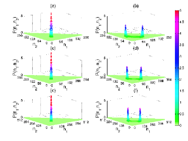
Figure 12: (color online). Varying number of particles for four wells: (a) Ground state and (b) entangled number state with $U=0.01E_{R}$ and $J=0.04e^{-\alpha}E_{R}$ with $\alpha=0.175$ for 256 particles at $t=1.74$ ms, 384 particles at $t=1.47$ ms, and 512 particles at $t=1.30$ ms in four wells for rows 1, 2, and 3. For the same barrier height, higher number of particles give rise to less extreme superpositions.

Our simulations indicate that entangled number states evolve through natural time evolution of the BEC with an initial phase offset of $\pi$ between the wells even with a large number of particles in each well. The extremity of the entangled number state can be controlled by varying the tunneling parameter or the number of particles.

V.2 Entangled number states in eight wells

Figure 13: (color online). 24 particles in eight wells: (a) Ground state and (b) entangled number state at $t=2.79$ ms for 24 particles in eight wells with $U=0.01E_{R}$ and $J=0.04e^{-\alpha}E_{R}$ with $\alpha=0.175$.

We present the dynamic creation of entangled number states in eight wells with just a few particles per well; this regime is similar to the regime studied by Greiner greiner2002 and we report our results using experimental parameters relevant to their work; ${}^{87}Rb$, $\lambda=852$ nm, $a_{sc}=5.8$ nm. Fig. 13 shows (a) ground state and (b) the time evolved entangled number state for 24 particles in eight wells with $J=0.04e^{-\alpha}E_{R}$ with $\alpha=0.175$ and $U=0.01E_{R}$ with an initial phase offset of $\pi$ between the wells. Our investigations show that entangled number states can also be realized in a larger number of wells with a small number of particles in each well.

V.3 Analysis of entangled number states: a new type of entangled state

The extreme entangled state for a multiwell BEC takes the form of Eq. 2. And the less extreme entangled states in multiple wells can have the approximate form

$$|\Psi\rangle_{\{N,M\}^{non-extreme}} = \frac{1}{\sqrt{M}}(|N-jn,n,\ldots,n\rangle$$ (14)

$$+|n,N-jn,n,\ldots,n\rangle$$

$$+\ldots+|n,\ldots,N-jn\rangle)$$

where $n<<N$ and $j=M-1$. The four well cat state shown in Fig. 8(b) is an extreme cat state in the approximate form $|\Psi\rangle=\frac{1}{\sqrt{4}}\left(|16,0,0,0\rangle+|0,16,0,0\rangle+|0,0,16,0\rangle+|0,0,0,16\rangle\right)$. An example of a less extreme cat state would be of the form $|\Psi\rangle=\frac{1}{\sqrt{4}}\left(|13,1,1,1\rangle+|1,13,1,1\rangle+|1,1,13,1\rangle+|1,1,1,13\rangle\right)$. Thus, one would expect a similar form for the large entangled states described in this section, however this is not what we found, as is shown below.

The states in Fig. 10 with the highest probability at $t=0$ and $t=2.40$ ms are shown in the first two entries of Table 1 and indicate there are 32 particles in each of the wells in the ground state and 57 particles simultaneously in all four wells in the entangled number state. The highest probability states in Fig. 11 with varying $J$ are shown in Table 1. Table 1 shows the ground states with the particles equally distributed between the wells and the entangled states with 57, 48, and 42 particles in all the wells. The highest probability states for Fig. 12 with varying $N$ are shown in Table 2, and Table 3 shows the highest probability states for the ground and entangled number states for the eight well system shown in Fig. 13. We would like to emphasize that the listed state is the highest coefficient state, and there are other lower coefficient states around this.

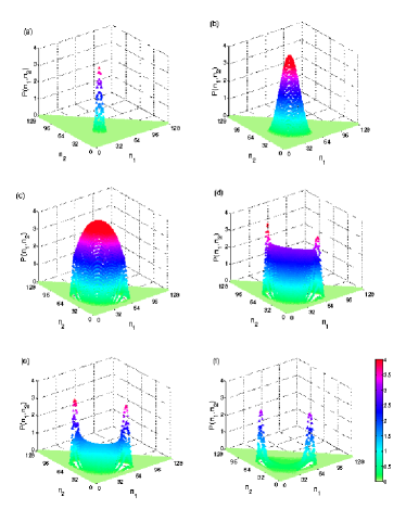
Figure 14: (color online). Evolution of entangled state for 128 particles in four wells, shown in the joint probability distribution space of Eq. 13 for sites 1 and 2. Shown are (a) at t=0, the ground state, (b) at t=1.22 ms, the ground state broadens, (c) at t=1.71 ms, (d) at t=1.84 ms the state is beginning to split just as it does in a double well and triple well, (e) at t=1.96 ms, and (f) at t=2.42 ms, the final entangled state is formed. The evolution here further illustrates that the underlying physical mechanism for the creation of cat states is the same in a double well and multiple wells.

Table 1: Highest probability states for 128 particles in four wells with $U=0.01E_{R}$ and varying $J$, where $J=0.04e^{-\alpha}E_{R}$. These states correspond to Fig. 11. It should be emphasized that all the Tables in this article show only the highest state; however, there are other non-vanishing coefficients as well as evident from Fig. 11. Those coefficients are smaller and spread out around the highest probability peak.

t (ms)	$\alpha$	highest probability state
0.0	0.175	$|32,32,32,32\rangle$
2.4	0.175	$\frac{1}{\sqrt{2}}(|57,7,57,7\rangle+|7,57,7,57\rangle)$
0.0	1.175	$|32,32,32,32\rangle$
3.65	1.175	$\frac{1}{\sqrt{2}}(|48,16,48,16\rangle+|16,48,16,48\rangle)$
0.0	2.175	$|32,32,32,32\rangle$
5.7	2.175	$\frac{1}{\sqrt{2}}(|42,22,42,22\rangle+|22,42,22,42\rangle)$

Table 2: Highest probability states in four wells with $J=0.04e^{-0.175}E_{R}$, $U=0.01E_{R}$ and varying $N$. These states correspond to Fig. 12.

t (ms)	$N$	highest probability state
0.0	256	$|64,64,64,64\rangle$
1.74	256	$\frac{1}{\sqrt{2}}(|102,26,102,26\rangle+|26,102,26,102\rangle)$
0.0	384	$|96,96,96,96\rangle$
1.47	384	$\frac{1}{\sqrt{2}}(|143,49,143,49\rangle+|143,49,143,49\rangle)$
0.0	512	$|128,128,128,128\rangle$
1.30	512	$\frac{1}{\sqrt{2}}(|183,73,183,73\rangle+|73,183,73,183\rangle)$

Table 3: Highest probability states in eight wells with $J=0.04e^{-0.175}E_{R}$, $U=0.01E_{R}$. These states correspond to Fig. 13.

t (ms)	highest probability state
0.0	$|3,3,3,3,3,3,3,3\rangle$
2.79	$\frac{1}{\sqrt{2}}(|6,0,6,0,6,0,6,0\rangle+|0,6,0,6,0,6,0,6\rangle)$

Based on the empirical evidence of the entangled number states shown in this section we find the entangled number states for large $N/M$ and large $M$ tend towards the approximate form

$$|\Psi\rangle = \left(\frac{1}{\sqrt{2}}\right)|\frac{2N}{M}-n,n,\frac{2N}{M}-n,\ldots,n\rangle$$ (15)

$$+|n,\frac{2N}{M}-n,n,\ldots,\frac{2N}{M}-n\rangle$$

where $n<N$ and there are $\frac{2N}{M}-n$ particles simultaneously in all $M$ wells. We say ‘approximate form’ because although the highest probability state has this form, there are many non-vanishing coefficients as well with smaller amplitudes, and spread out around the highest probability peak. The initial parameters of the system and dynamics determines the relative amplitudes of the non-vanishing coefficients for the final entangled states generated in our model.

To our knowledge at the time of writing, number entangled states in the form of Eq. 15 have not been discussed elsewhere and represent a new type of entanglement. Well known entangled states include Greene, Horne, Zeilnger states greenberger1990 shown in Eq. 1 which for two wells and $N$ particles is an extreme entangled state of the form, $(1/\sqrt{2})(|N,0\rangle+|0,N\rangle$), also known as NOON states. Another type of state is the W-state dur00 , which for $N$ qubits has the form, $(1/\sqrt{N})(|10..00\rangle+|01..00\rangle+..+|00..01\rangle)$. Because of the ‘twin-like’ nature, we refer to the number entangled states of Eq. 15 as Siamese states. For the case of qubits, W state was found to be more robust than GHZ state. For multi-dimensional quDits, the Siamese states introduced here may have different properties than other forms of number entangled states. We have only shown here a way of generating such novel states with cold atoms in a lattice without yet knowing their properties.

Tables 4 and 5 illustrate the relationship between particle number and interaction energy and these new types of entangled states. Table 4 shows that when we increase the number of particles, the Fock state number distribution in the final evolved state slowly turn into twin-like states. Same observation can also be made from the increase of interaction parameter $U$. Since particle number increment is effectively an increase in effective interaction, these results complement each other. Since in the Bose-Hubbard model the properties are determined by the ratio of $U/t$, we can say that starting with a small value of tunneling or a high barrier (highly squeezed state) is a prerequisite for obtaining these states. This actually makes the distinction very clear for the four well results, since we have shown for double well and three well, that to get toward an extreme cat state limit we need to start in the opposite limit of low barrier (gaussian state).

Fig. 14 shows evolution of a four well state, for a twin-like state. In the graphical representation of two-site joint probability function, a twin-like state and a four-legged cat state cannot be differentiated. For that we look at the coefficients of different Fock states to verify that this is a twin-like state, with the highest probability state being $(|57,7,57,7\rangle$+$|7,57,7,57\rangle)$, with other non-vanishing coefficients that are smaller. Fig. 14 presents the general picture of how a four well state evolves – (a) shows the phase imprinted ground state, (b) and (c) shows the broadening of the Gaussian distribution, (d) and (e) shows the process of splitting into superpositions, and (f) shows the final evolved state. This entangled number state example is for 128 particles, and $U=0.01E_{R}$, $J=0.04e^{-\alpha}E_{R}$ with $\alpha=0.175$. Figure 14 can be compared with Figs. 4 and 6 for double well and triple well respectively. We see that the dynamics of entangled state generation in a double well and multiple well follow similar properties – a gaussian ground state once phase imprinted to an unstable equilibrium, evolves first by broadening the gaussian, and then slowly splitting symmetrically to a macroscopic superposition state.

The detailed mechanism whereby the entangled states of Eq. 2 cross over to the new type of entangled states, with alternating populations as observed here, is not fully understood. Nor it it obvious why other types of entanglement pairings and types of alternation do not seem to occur. However, the most likely explanation of the cross-over effect itself will simply involve the fact that the entangled states of Eq. 2 have the maximal possible energies for the system: the proposed types of phase engineering explored here simply do not lead, as $N$ and $U$ increase, to energies high enough to allow simple time evolution into entangled states of such high energy. In terms of the underlying classical phase space dynamics, we can say that the characteristics of the unstable equilibrium (0,0,0,$\pi$,$\pi$,$\pi$) (in the conjugate variables $n_{12}$, $n_{23}$, $n_{34}$, $\phi_{12}$, $\phi_{23}$, $\phi_{34}$) changes as $U$ and $N$ is increased. For the double well case we know that $UN/J>1$ makes the $\pi$-phase an unstable equilibrium, and stable otherwise. Similarly, here the combination of values of $U$ and $N$ changes the scenario and beyond a certain value of $UN$, a complicated phase space dynamics constrains the motion in phase space in such a way that only certain region is accessible. Since we have presented quantum dynamics of multi-well in this paper based on intuition from its semiclassical aspects without a detailed study of dynamics in the underlying classical phase space as was done for the double well mahmud2005 , we cannot quantify our findings.

Table 4: Highest probability states in four wells with $J=0.04e^{-\alpha}E_{R}$ with $\alpha=0.0$, $U=0.01E_{R}$ and varying $N$.

t(ms)	$N$	highest probability state
7.69	20	$\frac{1}{\sqrt{4}}(|20,0,0,0\rangle+|0,20,0,0\rangle+$
		$|0,0,20,0\rangle+|0,0,0,20\rangle)$
6.39	24	$\frac{1}{\sqrt{4}}(|23,0,1,0\rangle+|0,23,0,1\rangle+$
		$|1,0,23,0\rangle+|0,1,0,23\rangle)$
6.24	28	$\frac{1}{\sqrt{4}}(|26,0,2,0\rangle+|0,26,0,2\rangle+$
		$|2,0,26,0\rangle+|0,2,0,26\rangle)$
5.38	32	$\frac{1}{\sqrt{4}}(|27,0,5,0\rangle+|0,27,0,5\rangle+$
		$|5,0,27,0\rangle+|0,5,0,27\rangle)$
2.91	64	$\frac{1}{\sqrt{2}}(|32,0,32,0\rangle+|0,32,0,32\rangle)$
2.15	128	$\frac{1}{\sqrt{2}}(|59,5,59,5\rangle+|5,59,5,59\rangle)$

Table 5: Highest probability states in four wells with $J=0.04e^{-\alpha}E_{R}$ with $\alpha=0.0$, $N=32$ and varying $U$ with $U=u(0.01E_{R})$.

t(ms)	$u$	highest probability state
5.70	0.15	$\frac{1}{\sqrt{4}}(|32,0,0,0\rangle+|0,32,0,0\rangle+$
		$|0,0,32,0\rangle+|0,0,0,32\rangle)$
5.38	0.25	$\frac{1}{\sqrt{4}}(|27,0,5,0\rangle+|0,27,0,5\rangle+$
		$|5,0,27,0\rangle+|0,5,0,27\rangle)$
2.91	0.50	$\frac{1}{\sqrt{4}}(|18,0,14,0\rangle+|0,18,0,14\rangle+$
		$|14,0,18,0\rangle+|0,14,0,18\rangle)$
2.47	0.75	$\frac{1}{\sqrt{4}}(|17,1,13,1\rangle+|1,17,1,13\rangle+$
		$|13,1,17,1\rangle+|1,13,1,17\rangle)$
2.08	1.00	$\frac{1}{\sqrt{4}}(|16,2,12,2\rangle+|2,16,2,12\rangle+$
		$|12,2,16,2\rangle+|2,12,2,16\rangle)$
1.66	1.25	$\frac{1}{\sqrt{4}}(|14,2,14,2\rangle+|2,14,2,14\rangle)$

VI Conclusions

We have demonstrated phase engineering schemes for the generation of entangled number states in multiple wells. These states represent a superposition of particles in a large number of spatial locations – a multi-positional generalization of double well NOON states. It is shown that entangled number states can be evolved from phase imprinted ground states of BEC in multiple wells, and the number of particles participating in the entanglement can be controlled by varying the height of the barrier between the wells, controlling the rate of ramping, and/or the number of particles. The less extreme entangled number states, which we show how to create in a controlled way, represent macroscopic superposition states that are more robust to experimental conditions and particle loss. We demonstrated our scheme with small number of particles in a small lattice, large number of particles per well, as well as with a large number of wells. Our investigations for four wells revealed a new type of number entangled state where a twin like state is formed, which we refer to as Siamese states. We demonstrated a relationship between the particle number and interaction strength and the formation of these new types of entangled states.

The physical mechanism by which these states are generated can be understood in terms of the underlying semiclassical phase space. Ground state put on an unstable equilibrium splits the wavepacket symmetrically to create these states. We briefly describe our earlier work on double well mahmud2005 ; mahmudThesis to demonstrate this in the semiclassical phase space, and to motivate and generalize the study to larger number of wells and lattices. The significance of the phase imprint values of $2\pi/3$ for three wells, and $\pi$ for four wells is explained this way. For the initial phase difference between the neighboring wells required to create these states, we presented a novel series of formulae that is valid for any number of wells, even or odd.

The creation, characterization, and applications of multidimensional/multipositional Schrödinger cat states of atoms discussed in this article remain largely unexplored experimentally, and the theoretical ramifications of such states, should they be easily produced, are just emerging.

- (1) A. Einstein, B. Podolsky, and N. Rosen, Phys. Rev. 47, 777 (1935).
- (2) J. S. Bell, Speakable and Unspeakable in Quantum Mechanics (Cambridge Univ. Press, Cambridge, 1987).
- (3) R. Horodecki, P. Horodecki, M. Horodecki, and K. Horodecki,, Rev. Mod. Phys. 81, 865 (2009).
- (4) S. F. Huelga et al., Phys. Rev. Lett. 79, 3865 (1997); V. Giovannetti, S. Lloyd, L. Maccone, Phys. Rev. Lett. 96 010401 (2006);
- (5) L. Pezze and A. Smerzi, Phys. Rev. Lett. 102 100401 (2009).
- (6) C. Monroe, Nature 416, 238 (2002).
- (7) Z. Zhao et al., Nature 430, 54 (2004).
- (8) H. Haffner et al., Nature 438, 639 (2005).
- (9) J. A. Jones et al., Science 324, 1166 (2009).
- (10) O. Mandel, M. Greiner, A. Widera, T. Rom, T. W. Hansch, I. Bloch, Nature 425, 937 (2003).
- (11) J. Esteve, C. Gross, A. Weller, S. Giovanazzi, and M. K. Oberthaler, Nature 455, 1216 (2008).
- (12) W. Marshall, C. Simon, R. Penrose, and D. Bouwmeester, Phys. Rev. Lett. 91, 130401 (2003).
- (13) O Romero-Isart, M. L. Juan, R Quidant, and J. I. Cirac, New J. Phys. 12, 033015 (2010).
- (14) J. S. Bell, Physics 1, 195 (1965).
- (15) D. M. Greenberger, M. A. Horne, A. Shimony, and A. Zeilinger, Am. J. Phys. 58, 1131 (1990).
- (16) E. Schrödinger, Naturwissenschaften 23, 807 (1935).
- (17) J. R. Friedman et al., Nature 406, 43 (2000).
- (18) C. H. van der Wal et al., Science 290, 773 (2000).
- (19) T. Morimae, Phys. Rev. A 81, 010101(R) (2010).
- (20) N. J. Cerf, S. Massar, and S. Pironio, Phys. Rev. Lett. 89, 080402 (2002).
- (21) O. Morsch, M. Oberthaler, Rev. Mod. Phys. 78, 179 (2006); M. Leweinstein, A. Sanpera, V. Ahufinger, B. Damski, A. Sen, and U. Sen, Advances in Physics 56, 243 (2007).
- (22) M. Greiner, O. Mandel, T. Esslinger, T. W. Hansch, and I. Bloch, Nature 415, 39 (2002).
- (23) C. Orzel, A. K. Tuchman, M. L. Fensclau, M. Yasuda, and M. A. Kasevich, Science 291, 2386 (2001).
- (24) K. W. Mahmud, H. Perry, and W. P. Reinhardt, Phys. Rev. A 71,023615 (2005); K. W. Mahmud, H. Perry, and W. P. Reinhardt, J. Phys. B 36, L265 (2003).
- (25) K. W. Mahmud, Ph.D. Thesis, University of Washington (2004).
- (26) L. Amico, A. Osterloh, and F. Cataliotti, Phys. Rev. Lett 95, 063201 (2005); K. Henderson, C. Ryu, C. MacCormick and M. G. Boshier, New J. Phys. 11, 043030 (2009).
- (27) M. P. A. Fisher, P. B. Weichman, G. Grinstein, and D. S. Fisher, Phys. Rev. B 40, 546 (1989).
- (28) D. Jaksch, C. Bruder, J. I. Cirac, C. W. Gardiner, and P. Zoller, Phys. Rev. Lett 81, 3108 (1998).
- (29) M. A. E. Leung and W. P. Reinhardt, Comp Phys Comm, 177 (4), 348 (2007).
- (30) J. Dunningham and D. Hallwood, Phys. Rev. A 74, 023601 (2006); J. A. Dunningham, K. Burnett, R. Roth, and W. D. Phillips, New J. Phys. 8, 182 (2006).
- (31) A. Nunnenkamp, A. M. Rey, and K. Burnett, Phys. Rev. A 77, 023622 (2008).
- (32) P. W. Anderson, Lectures on The Many-Body Problem, Vol 2, Pages 113-135, Academic Press, 1964.
- (33) A. Smerzi, S. Fantoni, S. Giovanazzi, and S. R. Shenoy, Phys. Rev. Lett. 79, 4950 (1997); S. Raghavan et al., Phys. Rev. A 59, 620 (1999).
- (34) M. Albiez, R. Gati, J. Folling, S. Hunsmann, M. Cristiani, M. K. Oberthaler, Phys. Rev. Lett. 95, 010402 (2005);
- (35) K. Husimi, Proc. Physico-Math. Soc. Japan 22, 264 (1940); H. Lee, Phys. Rep. 259, 147 (1995).
- (36) J. Denschlag et al., Science 287, 97 (2000).
- (37) A. Micheli, D. Jaksch, J. I. Cirac, and P. Zoller, Phys. Rev. A 67, 013607 (2003).
- (38) F. Piazza, L. Pezze, and A. Smerzi, Phys. Rev. A 78, 051601 (2008).
- (39) A variety of array configurations have been studied, including linear and circular arrays. The trimeric linear array with differing has been studied by: P. Buonsante, R. Franzosi, V. Penna, Phys. Rev. Lett 90, 050404 (2003).
- (40) R. Franzosi and V. Penna, Phys. Rev. E 67, 046227 (2003).
- (41) S. Mossmann and C. Jung, Phys. Rev. A 74, 033601 (2006).
- (42) F. Trimborn, D. Witthaut, and H. J. Korsch, Phys. Rev. A 79, 013608 (2009).
- (43) T. F. Viscondi, K. Furuya, M. C. de Oliveira, EPL 90, 10014 (2010).
- (44) A. Polkovnikov, Phys. Rev. A 68, 033609 (2003); A. Polkovnikov, S. Sachdev, S. M. Girvin, Phys. Rev. A 66, 053607 (2002).
- (45) K. W. Mahmud, M. A. Leung, and W. P. Reinhardt, arXiv:cond-mat/0403002.
- (46) W. Dur, G. Vidal and J. I. Cirac, Phys. Rev. A 62, 062314 (2000).