X-ray Flares of EV Lac: Statistics, Spectra, Diagnostics

Abstract

We study the spectral and temporal behavior of X-ray flares from the active M-dwarf EV Lac in 200 ks of exposure with the Chandra/HETGS. We derive flare parameters by fitting an empirical function which characterizes the amplitude, shape, and scale. The flares range from very short ($<1\,\mathrm{ks}$) to long ($\sim 10^{4}\,\mathrm{s}$) duration events with a range of shapes and amplitudes for all durations. We extract spectra for composite flares to study their mean evolution and to compare flares of different lengths. Evolution of spectral features in the density-temperature plane shows probable sustained heating. The short flares are significantly hotter than the longer flares. We determined an upper limit to the Fe K fluorescent flux, the best fit value being close to what is expected for compact loops.

1. Introduction

Coronal activity is ubiquitous among late type stars of all classes: pre-main sequence, main sequence, evolved binaries, and even some single giants. Activity on main sequence stars is generally correlated with rotation rate except at the shortest periods where saturation occurs. Flaring is common among the coronally active stars (as defined by high X-ray band luminosity relative to the bolometric luminosity, $\log(L_{\mathrm{x}}/L_{\mathrm{bol}})\sim-4$ to $-3$). Nearly every sufficiently long (many kiloseconds) X-ray observation of coronal sources shows flares, as defined by a rapid increase in flux accompanied by a hardening of the spectrum and subsequent decay and softening. Flares are the most dynamic aspects of coronal activity and are possibly a significant source of coronal heating. From Solar studies, we know that flare mechanisms involve magnetic field reconnection, particle beams, chromospheric evaporation, rapid bulk flows, mass ejection, and heating of plasma confined in loops.

Many stellar activity studies have attempted to avoid flares in order to determine quiescent coronal properties such as emission measure distributions, elemental abundances, loop heights, and geometric distribution of active regions. Since flares are a phenomenon of magnetic reconnection thought to occur on small spatial scales, modeling the dynamic behavior allows us to constrain loop properties in ways that cannot be done from analysis of quiescent coronae that necessarily require a spatial and temporal average over a large ensemble of coronal structures. Use of rotational modulation of flux and velocity has become a common and important technique (Doppler imaging, and related methods) for mapping the stable and non-uniform structures of stellar activity. Flare modeling has the potential to become as important for determining the properties of transient loop structures and their energetics (e.g. Reale, 2007; Aschwanden & Tsiklauri, 2009).

Here we exploit the flaring behavior in EV Lac— one of the brightest, most reliable flaring sources available — to obtain spectra and temporal profiles in flares from Chandra X-ray Observatory (CXO) High Resolution Transmission Grating Spectrometer (HETGS) observations. The $200\,\mathrm{ks}$ exposure, flare frequency, and amplitudes are sufficient to provide spectral diagnostics in flares if we combine multiple events to examine the mean properties of emission line and continuum evolution. In addition, we study the distribution of flare temporal morphologies.

Even though EV Lac has a high flare rate, we are still forced to work with some mean quantities by combining data from multiple, possibly physically different flares. Nevertheless, the results are interesting and are necessary groundwork for guiding future studies. In this paper, we characterize the flares and present some simple diagnostics from different flare states. We also model Fe K fluorescence. Detailed hydrodynamic models will be applied in future work.

1.1. Characteristics of EV Lac

EV Lac is a nearby (5 pc) dM3.5e ($0.35M_{\odot}$, $0.36R_{\odot}$) flare star with a photometric period of 4.4 days. It is among the X-ray brightest of single dMe flare stars (Robrade & Schmitt, 2005), having a mean $L_{\mathrm{x}}\sim 3-5\times 10^{28}\,\mathrm{ergs\,cm^{-2}\,s^{-1}}$. It is of particular interest for this study for these specific reasons:

$\bullet$ EV Lac has consistently shown frequent and strong flares whenever observed in X-rays, as has been demonstrated with $ROSAT$ and $SAX$ (Sciortino et al., 1999), $ASCA$ (Favata et al., 2000), $XMM/Newton$ (Mitra-Kraev et al., 2005; Robrade & Schmitt, 2006), $Chandra$ (Osten et al., 2005), and Suzaku (Laming & Hwang, 2009). Models imply that the flaring structures are of a compact nature. Such a compact geometry is more efficient for producing Fe K fluorescent emissions due to the larger solid angle seen by the photosphere, and also because lower loop heights have a greater the yield of Fe K photons from the fluorescing photosphere — more hard X-ray photons enter at small angle and have a lower optical depth for escape (Bai, 1979). The X-ray flare frequency is about $0.4\,\mathrm{hr^{-1}}$ (see Figure 1), similar to previously quoted rates of $0.2-0.3\,\mathrm{hr^{-1}}$ for X-ray, UV, and U-band flares (Osten et al., 2005; Mitra-Kraev et al., 2005). Some of the flares are very short ($\leq 1\,\mathrm{ks}$; Figure 1 and Osten et al. (2005)). The short duration attests to a compact size since larger volumes have longer cooling times due to their lower density which reduces the radiative and conductive loss rates. With the addition of the new HETG observations, we have identified 25 flares in $200\,\mathrm{ks}$ (Figure 1), with a broad range in amplitude and timescales.

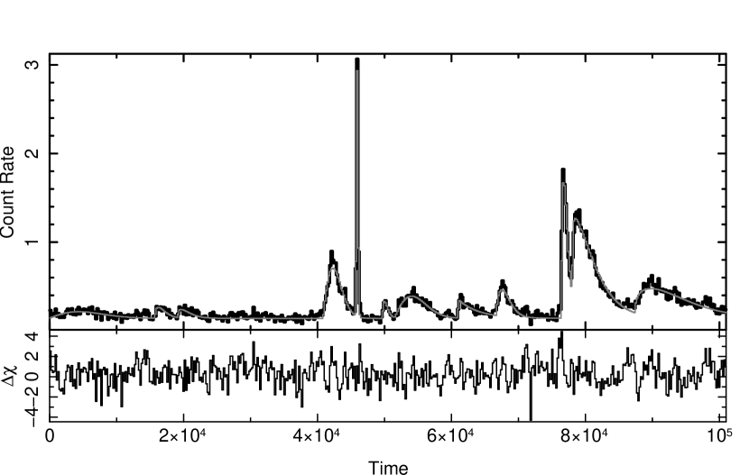
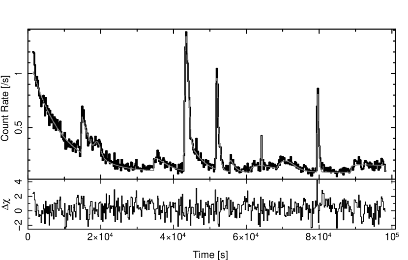
Figure 1.— These are the light curves from the two HETGS observations, for HEG and MEG $1-25\,\mathrm{{\AA}}$ events. The top shows the 2001 observation (ObsID 1885), and bottom 2009 (ObsID 10679). It is clear that flares are frequent; 25 were identified and fit with an empirical function, for which we show the model (overlayed smooth, light-colored curve) and residuals (lower panels).

$\bullet$ EV Lac’s O vii triplet ratio showed a density of about $6\times 10^{10}\,\mathrm{cm}^{-3}$ (Testa, Drake & Peres, 2004; Ness et al., 2004). The ability to measure density provides strong constraints on the emitting volume.

$\bullet$ EV Lac is one of 3 in a sample of 22 coronally active stars which showed presence of opacity as determined from the ratios of H-like Ly$\alpha$ to Ly$\beta$ resonance lines (Testa et al., 2007a). Measurement of opacity can also provide constraints on emitting structure geometry. Testa et al. (2007a) derived a compact coronal height of about 0.06 stellar radii.

$\bullet$ EV Lac has a strong and variable magnetic field ($3\,\mathrm{kG}$) with about a 50% surface filling factor (Johns-Krull & Valenti, 1996; Phan-Bao et al., 2006), and it was both poloidal and asymmetric (Donati et al., 2008). Strong fields may be necessary for forming and maintaining compact loops which give rise to the short, energetic flares. The star is near the expected mass boundary for transition from an $\alpha-\omega$ dynamo to a turbulent dynamo and so could be an important case theoretically.

2. Chandra/HETGS Observations and Data Processing

Chandra has observed EV Lac twice with the HETGS, once in 2001 (Observation Identifier 1885) for $100\,\mathrm{ks}$, and once in 2009 (ObsID 10679, as part of the HETG Guaranteed Time Observation program) for $97\,\mathrm{ks}$. The spectrometer and observatory are described by Canizares et al. (2005) and Weisskopf et al. (2002), respectively. The observational data were processed with the standard software suite, CIAO (Fruscione et al., 2006) to filter, transform, bin spectra, and construct the observation-dependent responses. These CIAO programs were in turn driven by the TGCat (Mitschang, Huenemoerder & Nichols, 2010) reprocessing scripts which automates the CIAO processes into an end-to-end pipeline. This was especially useful for extraction of hundreds of spectra and responses in time-filtered intervals (see §4). Light curves were binned from the event files using the “ACIS Gratings Light Curve” package (aglc), which bins counts and count rate light curves over multiple detector chips, grating orders, grating types, and wavelength regions of the dispersed grating spectrum.

3. Flare Light Curve Fitting & Statistics

The Weibull distribution is a convenient function for empirically fitting the shapes of the flares, whether impulsive or gradual. The normalized distribution is

$$f(p;a,s)= \left(\frac{a}{s}\right)p^{(a-1)}e^{-p^{a}}$$ (1)

$$p= (t-t_{0})/s$$ (2)

in which $a$ is a shape parameter ($a>0$), the decay scale (or width of the distribution) is specified by $s$ ($s>0$), the offset is given by $t_{0}$ ($t_{0}\geq 0$); the independent time coordinate is $t$ ($t\geq t_{0}$). Shapes $a\leq 1$ are exponential-like — there is no resolved rise. A shape $a>1$ is more Gaussian-like, becoming more symmetric as $a$ increases. For $a<1$, the function falls faster than an exponential, and for $a>1$, it falls somewhat slower than an exponential, up to a factor of about 1.5, as defined by the $e$-folding time from the peak rate.

Light curves were binned to $100\,\mathrm{s}$ using events from positive and negative first orders, HEG and MEG, from $1.5$–$25\,\,\mathrm{{\AA}}$. These uniformly-binned light curves were fit iteratively using a sum of Weibull distributions scaled by an amplitude parameter, and including a constant basal count rate; in other words, we fit $Af(p;a,s)+R_{0}$ in which $A$ is the flare area in counts, $R_{0}$ the baseline rate in $\,\mathrm{cts\,s^{-1}}$ for the observation, and $f$ is given by equations 1-2. We first defined model components for obvious flares, fitting the region of significantly overlapping flares, and then added components as required to flatten the residuals. Since we physically expect single-loop flares undergoing radiative decay to be exponential in time, or likely prolonged by sustained heating, we constrained the shape, $a$, to be $\geq 1$ so that the decay is exponential or slower.

Table 1Flare Light Curve Fit Parameters

$n$	$area$	$t_{0}$	$a$	$s$	$\tau_{1}$	$\tau_{2}$	$r$
	[cts]	[s]	-	[s]	[s]	[s]	[cts/s]
(1)	(2)	(3)	(4)	(5)	(6)	(7)	(8)
101	595 (494, 713)	0 (0, 524)	1.89 (1.46, 2.47)	6474 (5691, 7857)	9818	4346	0.08
111	234 (183, 292)	15685 (15685, 15785)	1.40 (1.04, 1.77)	1383 (1047, 1833)	2116	563	0.12
112	226 (170, 281)	19101 (19101, 19202)	1.32 (1.00, 1.75)	1715 (1304, 2144)	2586	588	0.10
102	1533 (1452, 1614)	40861 (40747, 40904)	1.85 (1.72, 2.02)	2181 (2068, 2316)	3320	1432	0.57
103	854 (802, 905)	45726 (45721, 45726)	2.13 (2.00, 2.30)	239 (230, 250)	354	177	3.18
104	184 (138, 232)	49645 (49486, 49745)	1.47 (1.02, 2.81)	698 (508, 866)	1076	321	0.20
105	1154 (1073, 1237)	51548 (51548, 51926)	1.89 (1.55, 2.05)	3752 (3358, 3954)	5689	2517	0.25
106	675 (554, 802)	60934 (60898, 60998)	1.00 (1.00, 1.13)	3100 (2322, 4115)	3104	0	0.22
107	666 (586, 749)	66725 (66642, 66825)	1.53 (1.33, 1.72)	1659 (1462, 1840)	2563	834	0.30
108	1753 (1669, 1840)	76370 (76364, 76370)	1.45 (1.38, 1.52)	819 (777, 868)	1260	366	1.58
109	4639 (4492, 4786)	78078 (78065, 78078)	1.19 (1.15, 1.22)	3264 (3140, 3397)	4627	682	1.08
110	3089 (2928, 3260)	87418 (87255, 87422)	1.38 (1.31, 1.47)	7105 (6681, 7611)	10839	2776	0.32
9	7742 (7436, 9336)	1305 (0, 1371)	1.00 (1.00, 1.01)	8071 (7652, 8529)	8084	0	0.96
8	1052 (725, 1292)	14639 (14538, 14639)	1.01 (1.00, 1.36)	2738 (1505, 3429)	2912	33	0.36
10	200 (123, 450)	17654 (17300, 18358)	2.45 (1.00, 4.81)	1895 (1082, 2855)	2724	1528	0.10
4	537 (454, 645)	34448 (34261, 34540)	1.19 (1.01, 1.44)	3501 (2853, 4718)	4988	761	0.12
1	1291 (1140, 1416)	42782 (42664, 42783)	1.24 (1.15, 1.44)	3804 (3366, 4469)	5575	1024	0.25
12	1154 (1035, 1296)	42969 (42891, 42984)	1.71 (1.56, 1.99)	890 (827, 994)	1369	533	1.02
2	760 (702, 818)	51628 (51601, 51628)	1.24 (1.16, 1.33)	616 (563, 674)	904	167	0.92
3	166 (127, 232)	55447 (55347, 55548)	1.16 (1.00, 1.51)	1202 (898, 2009)	1664	212	0.11
13	547 (428, 691)	60975 (60900, 61478)	1.42 (1.09, 1.71)	6547 (5303, 8475)	10046	2787	0.06
7	71 (50, 181)	64091 (63982, 64091)	1.27 (1.00, 3.33)	142 (100, 225)	210	42	0.37
6	406 (304, 511)	68413 (67939, 68814)	1.81 (1.46, 2.47)	3918 (3294, 4760)	5981	2512	0.08
5	436 (397, 475)	79369 (79354, 79369)	1.57 (1.45, 1.72)	424 (390, 460)	655	224	0.78
11	2246 (1012, 63190)	88716 (88315, 88918)	1.12 (1.00, 1.28)	25389 (10008, 278646)	33882	3459	0.07

Note. — The central horizontal line separates the 2001 and 2009 observations. Parameters $t_{0}$, $a$, and $s$ are as defined by Equations 1-2, and the $area$ is the flare amplitude. The index $n$ is an arbitrary identifier (with no significance to the order); it is used to mark the flares displayed in Figure 3. The vertical line separates the fitted parameters from some derived parameters which may be more intuitive. Values in parentheses are $90\%$ confidence limits.

Table 1 gives the flare parameters. The first column, $n$, is an arbitrary index used as a unique identifier for each flare (with no significance to the order). The second column, $area$, is the overall normalization, or amplitude, of the flare in counts, integrated over $1$–$25\,\mathrm{{\AA}}$. The next three columns (3–5) give the Weibull distrubution’s parameters, $t_{0}$, the flare start time (measured from the start of the observation), the shape parameter, $a$, and the scale parameter, $s$. The values in parentheses are the $90\%$ confidence intervals of the parameters.

The last three columns (6–8) are not independent parameters, but are given as an alternate and more familiar characterization of the flares. They are the $e$-folding time from the peak, $\tau_{1}$, the lag from the start to the peak, $\tau_{2}$, and the count rate at the peak, $r$. The horizontal line midway down the table separates the 2001 observation ($n>100$) from that of 2009. Figure 2 shows the shapes, scales, and areas graphically. The baseline count rates, $R_{0}$ were slightly different for the two observations, being $0.151\,(0.004)$ in 2001, and $0.092\,(0.002)$ in 2009 (uncertainties are for 90% confidence).

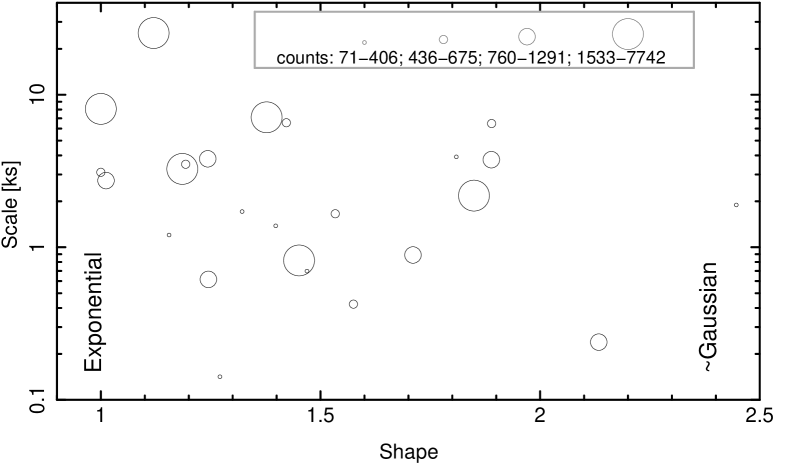
Figure 2.— Flare fit parameters. These specify the model used in Figure 1 and listed in Table 1. A $shape$ ($a$) of 1 means exponential decay, while larger shapes have resolved rises. The $scale$ ($s$) is approximately the $e$-folding time from the peak rate. Circles’ radii are proportional to the $\log$ of the flare counts, grouped in quartiles (the inset key gives actual ranges in counts). There is no obvious correlation among these parameters.

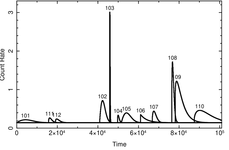
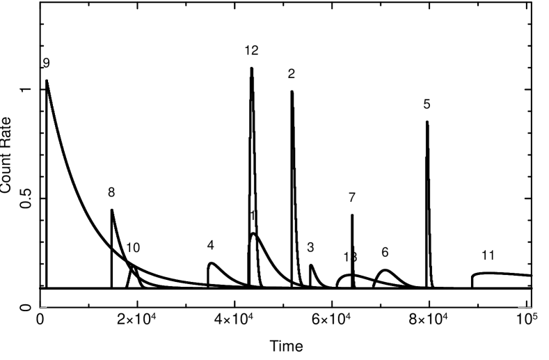
Figure 3.— These are the model components for each flare, with the index, $n$, as given in Table 1.

4. Flare Spectral Profile Extraction & Fitting

In order to get enough counts in different flare states, we need to extract spectra as a function of time during flares, then form composite spectra from states deemed similar. Time ranges and number of spectra to extract were identified manually from the light curves, using higher time resolution during intervals of more rapid change. Given a list of start times, stop times, and number of spectra, good-time-interval (GTI) tables were constructed which were then used to filter the events and extract spectra. We extracted 121 spectra for the 2001 observation, and 118 for 2009. Processing was automated using the tgcat scripts so that each spectrum also has the appropriate response for its time interval.

Given the extractions, the flare phase of each time bin was then defined as “low”, “rise”, “peak”, “decay high”, “decay low”, or “ignore”. Of the 249 total spectra extracted (each comprised of HEG and MEG positive and negative first orders), 109 were assigned to the noticed groups, the ignored remainder being of ambiguous phase due to overlapping flares of comparable magnitude. Table LABEL:tbl:flarestatestats gives some summary statistics on the selections. Since the rises are often very sharp, we have the shortest exposure and fewest counts in this group. The longest time bin, for the low phase, was $17\,\mathrm{ks}$, while during flares we used bins as short as $300\,\mathrm{s}$. In Figure 4 we show detail of some of the flare phase selections.

Table 2Flare Phase Information

Phase	$N$	$t_{\mathrm{exp}}$	Counts
		[ks]
low	13	50	7235
rise	15	9	3036
peak	21	10	8133
decay-high	26	18	10585
decay-low	34	22	7369
$N$ is the number of spectra extracted in each flare phase.

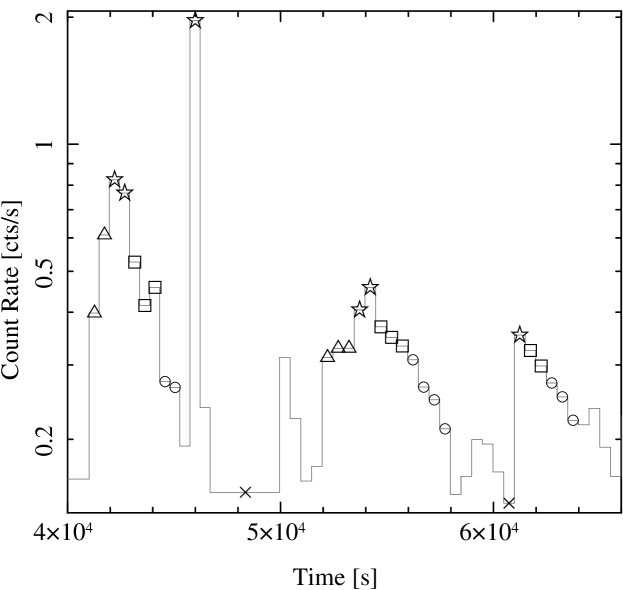
Figure 4.— Here we show detailed evolution for flares 104–106, events with resolved rise and decay, no resolved rise, or only the unresolved peak. We define the flare “phases” as the rise (triangles), peaks (stars), decay-high (squares), decay-low (circles), and low (crosses).

The spectral analysis fitting was done by loading the individual spectral counts histograms and their associated response files into the ISIS (Houck, 2002; Houck & Denicola, 2000) analysis system where they could then be associated and combined dynamically during fitting. Spectral grouping was also done dynamically as appropriate to obtain sufficient statistics per wavelength bin.

5. Flare Modeling

We study the flares by applying different model approaches to derive diagnostics at different levels, using Solar flare models as a basis. The numerical models have become very sophisticated; codes and methods have been tested in detail against spatially resolved solar observations (see for examples, Reale, 2007; Klimchuk, Patsourakos & Cargill, 2008; Aschwanden & Tsiklauri, 2009). In application of these models to EV Lac flares coupled with spectral diagnostics, we can potentially constrain flare loop conditions in this M-dwarf and relate it to the Sun and other stars.

Many solar X-ray flares are characterized by simple rise plus decay light curves and typically involve localized loop structures, where the plasma is confined by the coronal magnetic field. It is then possible to describe the flaring plasma as a compressible fluid which moves and transports energy along the magnetic field lines and use time-dependent hydrodynamic models. In these conditions, it has been shown that the flare decay time scales with the length of the flaring loop (Serio et al., 1991) and the presence of significant heating in the decay can make the decay longer than expected (Jakimiec et al., 1992; Sylwester et al., 1993). Such heating can be diagnosed from the analysis of the flare path in the density-temperature diagram: the flare decay path becomes shallower. From numerical modeling, scaling laws have been derived to estimate the loop length after correcting for the effect of heating (Reale et al., 1997): $L_{9}=C\,\tau_{\mathrm{x}}\sqrt{T_{7}}$, where $L_{9}$ is the loop half length ($10^{9}\,\mathrm{cm}$), $\tau_{\mathrm{x}}$ the decay time of the X-ray light curve in seconds, $T_{7}$ is the maximum flare temperature ($10^{7}\,\mathrm{K}$), and $C$ a proportionality factor. Such a diagnostic tool is well established and has been commonly applied to analyze stellar flares (Reale & Micela, 1998; Favata & Schmitt, 1999; Maggio et al., 2000; Stelzer et al., 2002; Briggs & Pye, 2003; Pillitteri et al., 2005; Favata et al., 2005). Without heating, the scale factor $C=1/120$ (Serio et al., 1991), but the scaling law can greatly overestimate the loop length. More recently, new diagnostic tools have been developed to obtain information on the flaring plasma and structures from the flare rise phase (Reale, 2007). It has been also shown that flares with more complex light curves, e.g. with multiple peaks, can involve more coronal loops (Reale et al., 2004).

We are limited by statistics to composites of heterogeneous flare types. Nevertheless, the behavior agrees in general with theoretical expectations. Since no single flare is strong enough for this analysis, we combined spectra from several flares and provide diagnostics for both lines and continua. One theoretically interesting diagnostic is the evolution of temperature and density (or its proxy, $\sqrt{EM}$). The helium-like to hydrogen-like line ratios are a strong function of temperature. From a portion of the spectrum which includes a line pair, we can derive a characteristic temperature and emission measure from a relatively simple, single-temperature APED model fit. Figure 5 shows the Si xiv–Si xiii region.

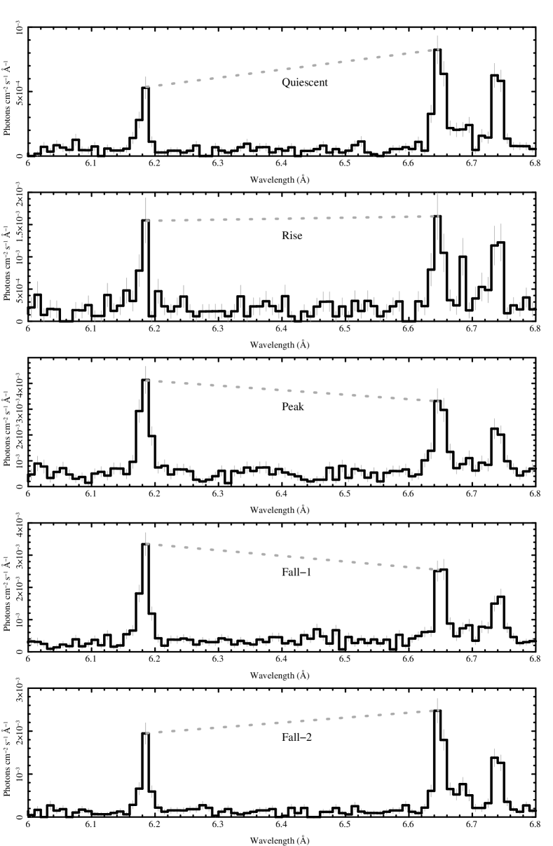
Figure 5.— This figure shows the evolution of the He-like Si xiv ($6.18\,\mathrm{{\AA}}$) to Si xiii ($6.65\,\mathrm{{\AA}}$) line fluxes through a composite flare. Note that the $y$-axes have very different scales.

We have derived temperatures from fits to several H-like to He-like line pairs and a $3-6\,\mathrm{{\AA}}$ continuum band using APED emissivities. Figure 6 shows the results for many flares in the existing data, grouped by flare phase as given in Table LABEL:tbl:flarestatestats. These agree qualitatively with paths expected from single-loop theory (Reale, 2007). The initial low-phase is the left-most point for each feature, and flare phase (or time, if it were a single flare event) proceeds (generally) clockwise around the loop. This is similar to results of Testa et al. (2007b) on a single, large flare in the active giant, HR 9024. Figure 6 also shows two arbitrarily placed lines, one of slope 2, and the other of slope $1/2$. The former is characteristic of radiative and conductive decay, and the latter of quasi-steady-state conditions in which the heating changes slowly enough that the temperature and density can obtain their equilibrium values in a hydrostatic magnetic “RTV” (Rosner, Tucker & Vaiana, 1978) loop. (For details on such hydrodynamic model trajectories, see Jakimiec et al. (1992); Reale (2007); Sylwester et al. (1993).) The measurements shown for EV Lac generally have slopes between these limits, implying that our flare composite has some sustained heating. The fact that some of the lines cross (e.g., for Si and Mg) likely means that we have mixed flares of very different physical characteristics, and that we require finer grouping by flare types (and consequently, better statistics).

The temperatures at identical phases differ between spectral features because we are sampling from plasma with a distribution of temperatures, and the features have different emissivity dependence upon temperature. In Figure 6, if we were to connect the points at identical phases, then we would have a crude emission measure distribution with temperature (in the square root, and vertically oriented) for each flare phase.

The naive scaling law for the range in peak temperatures seen ($T_{7}\sim 0.6-3.0$) and broad range in decay scales ($200-30000\,\mathrm{s}$) would imply a huge range in $L_{9}$, of two orders of magnitude, $\sim 1$–$100$. However, we know that we have a heterogeneous mix and that there is sustained heating, so the upper value is clearly a gross overestimate (for reference, the stellar radius in these units is 25). If we consider only the shortest flares — which are more likely to occur in one or few loops — then the range is a more plausible $L_{9}\sim 0.1-1$.

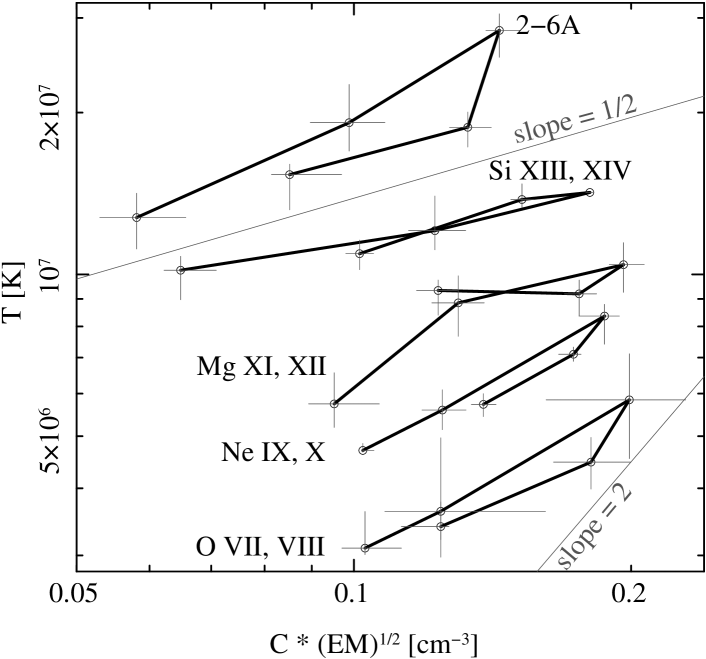
Figure 6.— Evolution of temperature and density proxy using several line pairs or a continuum band for the composite flare phase selections. The line flux and temperature diagram traces the evolution of a flare, using composite spectra from different phases of many flares. The 5 points on each curve correspond to the different flare phases, as defined in Table LABEL:tbl:flarestatestats, starting from the low phase at the left-most point in each case and proceeding through “rise”, “peak”, “decay-high”, and “decay-low”. When combined with time-dependent hydrodynamical flare models, the slopes in the different phases can be related to flare loop sizes and heating functions. We show two limits as gray lines — a slope of 2 is characteristic of radiative and conductive decay, and a slope of $1/2$ of quasi-steady-state decay. Errorbars are the 90% confidence limits from the single-temperature APED fits to each spectral region.

Further progress will likely require us to obtain better statistics in groups of similar flares, in order to constrain loop parameters with hydrodynamic models. For instance, due to limited time resolution, we are not certain that the temperature and density peak at the same flare phase, as they appear to do in Figure 6. If we had better temporally-resolved spectra for several similar flares (shape and duration), then we could apply detailed hydrodynamic modeling by solving accurately the time-dependent hydrodynamic plasma equations with the aid of the Palermo-Harvard numerical code (Peres et al., 1982; Betta et al., 1997). This approach allows one to obtain deeper insight into the flaring plasma and of the heating details, such as the detailed thermal structure and its evolution, and information about the loop aspect (Reale et al., 2004; Favata et al., 2005; Testa et al., 2007b). Such will be attempted in future work, and hopefully with a larger dataset which supports grouping of more like events.

5.1. Spectral Comparison of Different States

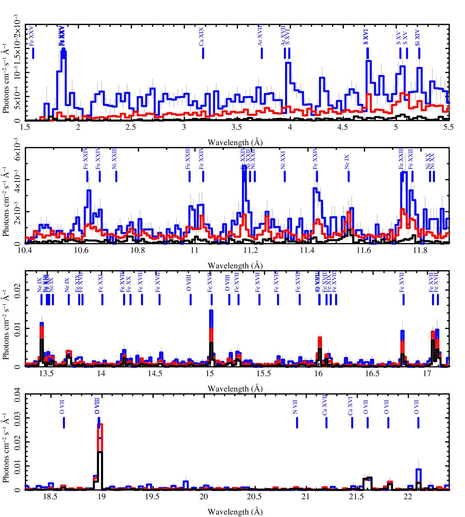
Figure 7.— Photon flux density spectra for different states in a few wavelength ranges: short flares (upper curves; blue), long flares (middle curve; red), and the low phase (lowest curve; black). These are “unfolded” spectra, in which the effective area has been factored out, but the instrumental line-spread-function remains. The short flare curve has more noise since it has the shortest exposure of $7\,\mathrm{ks}$. The others have $42\,\mathrm{ks}$ (long flares) and $50\,\mathrm{ks}$ (quiescent) exposures. Positions of some features (not all actually present) have been marked. The flare spectra have been integrated over their durations.

Figure 8.— The three-component APED fit parameters show the changes in temperature ($x$-axis) and emission measure ($y$-axis) for the short flares (circles), long flares (stars) and low phase (squares) spectra. The short flares are clearly much hotter than the long.

We can empirically compare spectra for the short and long flares to each other and to the low, or “quiescent” phase. We have extracted spectra integrated over the flare duration for short flares (flare numbers 2, 5, 7, 12, 103, 104 and 108; see Figure 3), long flares (numbers 4, 6, 8, 9, 10, 102, 105, 109, 110), and for low phases. In these groups, we respectively have exposures of $7\,\mathrm{ks}$, $42\,\mathrm{ks}$, and $50\,\mathrm{ks}$. To characterize the spectra, we have fit a 3-component APED model to each. Such a model is not as definitive as a line-based emission measure and abundance reconstruction. The temperature represents some average value since the line features can change dramatically over temperature differences of order of a factor of 2, which a 3-temperature model cannot fairly represent over the broad range of plasma temperatures. Also, the abundances are largely another line-strength parameter which can compensate for off-nominal temperatures as well as real abundance values; we do not consider abundance to be an interesting parameter for this purpose (determination of meaningful abundances requires line-based emission measure reconstruction). Nevertheless, the model is sufficient to show the primary differences between the phases. The short wavelength continuum ($<6\,\mathrm{{\AA}}$) constrains the highest temperature component, while the lines, primarily the H-like and He-like series, constrain the lower temperature components. Some lines, such as Fe xxiv can also have a significant effect at the high temperatures of flares.

In Figure 7, we show the three different spectra for different wavelength intervals. The upper (at the shorter wavelengths) curve (blue) shows the short flares’ peak phase. It is somewhat noisier than the other two curves due to its lower exposure, but is systematically stronger and has features characteristic of high temperature which are weaker or not present in the long flare (red middle curve) or quiescent (black lowest curve) states. Fe xxv and the S xv-S xvi series are prominent during the short flares (upper panel), as are other high ionization states of iron, such as Fe xxiii and Fe xxiv (second panel). At longer wavelengths (lower two panels), where low temperature features dominate, changes are less pronounced.

In Figure 8 we show the temperature versus emission measure from the three-component APED fits. It is clear that the shortest flares have much greater weight in the hottest plasma than the long flares. The long flares do have some high temperature plasma, but it does not dominate the emission measure. Their greater weight in cooler plasma during the decay implies that the emission originates from a multi-loop flaring system with simultaneous cooling and heating (Reale, Bocchino & Peres, 2002; López-Santiago et al., 2010). The sustained heating produces more hot plasma, which then cools and thereby enhance the cooler region of the emission measure distribution. The short, hot flares probably occur in single or few loops, and being short, do not ultimately provide as large a volume of plasma in the cooler state.

We should note again the limitations of the three-temperature fit: the short flare spectra do have emission from lower temperature ions such as O vii, O viii, and Fe xvii (see Figure 7), and so there should be some fourth point in the Figure 8 “Short” curve at low temperatures ($2$-$3\,\mathrm{MK}$) with significant emission measure. Such will be addressed in future work through detailed emission measure reconstruction.

6. Fe K Fluorescence

At present only the solar corona can be studied in spatial detail. Fluorescent lines provide a powerful spectroscopic method for probing flare geometry for the unresolved coronae of more distant stars. X-rays of energy $\gtrsim 7\,\mathrm{keV}$ emitted from a hot corona incident on the underlying photosphere are predominantly destroyed by photo-absorption events through inner-shell ionization of atoms or weakly ionized species. Observable fluorescent lines arise from photons emitted in outward directions by the $2p-1s$ decay of the excited atom. In a plasma with solar-like composition, only Fe fluorescent lines are expected to be detected (Bai, 1979; Drake, Ercolano & Swartz, 2008). The fluorescent line equivalent width depends on the height of the X-ray source above the photosphere and the heliocentric angle between the flare and line-of-sight. Line strength also depends on the relative photospheric Fe abundance but is independent of global metallicity except for very metal-poor stars. For coronal scale heights $>0.5R_{\star}$ the Fe K line becomes very weak owing to geometric dilution and the larger mean angle of incidence. The Fe K line is thus potentially a very powerful diagnostic of flare geometry and location; it can both constrain and calibrate physical models of flares.

In the first detailed study of this kind, Fe K fluorescence was produced by a single large flare in the HETGS observation of the active giant HR 9024. Testa et al. (2007b) found the origin compatible with photospheric photospheric heights and inferred a very compact scale height of $\leq 0.1\,R_{\star}$. A prominent Fe K fluorescent line was recently observed from a super flare on the RS CVn-like binary II Peg by Osten et al. (2007) who found the line to be surprisingly strong for photospheric fluorescence. Osten (2010) detected a very large flare on EV Lac with Swift, with a peak Fe K$\alpha$ flux of $0.027\,\mathrm{photons\,cm^{-2}s^{-1}}$. Their analysis obtained consistent results from fluorescence and hydrodynamic models, with a compact loop of height about $0.2R_{*}$.

Based on their rapid decay, the short flares seen from EV Lac are expected to be small, single-loop events, and hence efficient producers of Fe K fluorescence from the underlying photosphere (Ercolano, Barlow & Storey, 2005). To search for this fluorescence signature, we combined spectra from multiple short flares. The 90% confidence upper limit to the Fe K flux is about $6\times 10^{-5}\,\mathrm{phot\,cm^{-2}s^{-1}}$. Given our estimate of the $7$–$20\,\mathrm{keV}$ flux and the continuum intensity in the vicinity of the Fe K line, the expected equivalent width is $\sim 150$ eV for compact flares computed by Drake, Ercolano & Swartz (2008), corresponding to an Fe K flux of about $2\times 10^{-5}\,\mathrm{phot\,cm^{-2}s^{-1}}$. Figure 9 shows our fit to the flaring spectrum. A more sensitive observation is required in order to provide useful constraints from fluorescence on the flare scale height. We estimate for double the exposure in short flares ($14\,\mathrm{ks}$), we can detect a flux of $2\times 10^{-5}\,\mathrm{phot\,cm^{-2}s^{-1}}$ at 90% confidence.

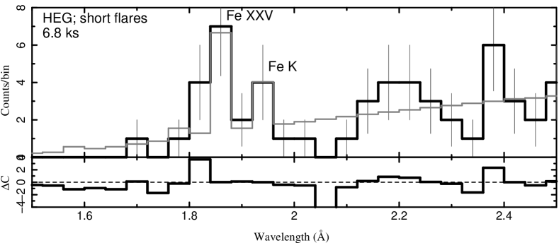
Figure 9.— Our current composite flare peak spectrum for $7\,\,\mathrm{ks}$ of short flares (dark histogram with light error bars) and best fit model (light curve). The best fit to Fe K gives a flux of $2\times 10^{-5}\,\mathrm{photons\,cm^{-2}\,s^{-1}}$, and a 90% confidence upper limit of $6\times 10^{-5}\,\mathrm{photons\,cm^{-2}\,s^{-1}}$.

7. Conclusions

We have shown that EV Lac is a reliable factory of X-ray flares, and that they come in a large range of shapes and sizes, from time scales of $\sim 100\,\mathrm{s}$ to over $10^{4}\,\mathrm{s}$, and a similar range in integrated HETG counts. However, their typical brevity and amplitude precludes study of spectral evolution for any single flare, so we have resorted to modeling of composite flares. The evolution of temperature and emission measure obtained from line emission does indicate that there is sustained heating and that simple loop model scaling laws are probably inappropriate. The short flares seem qualitatively different from the long flares in their highest weight for the hottest plasma. If we assume that there is no sustained heating in these flares, then the simple scaling laws would imply longer loops due to their higher temperatures, but the short timescale imply shorter loops. The simple scaling law (see §5) gives $L_{9}\sim 3-21$, roughly 0.1 to 1 stellar radius, a plausible range. Given the diversity of flare shapes and scales, we estimate that it would take an additional $200\,\mathrm{ks}$ observation to provide sufficient statistics in similar moderate length flares for detailed hydrodynamic modeling of spectral evolution, and also enough counts in short flares to provide a positive detection of Fe K fluorescence, and thus provide two independent determinations of loop sizes.

Facilities:

CXO (HETGS)

Acknowledgments

Support for this work was provided by the National Aeronautics and Space Administration through the Smithsonian Astrophysical Observatory contract SV3-73016 to MIT for Support of the Chandra X-Ray Center and Science Instruments, which is operated by the Smithsonian Astrophysical Observatory for and on behalf of the National Aeronautics Space Administration under contract NAS8-03060. JJD and PT acknowledge support from the Chandra X-ray Center NASA contract NAS8-03060. We thank Prof. Claude Canizares for granting HETG/GTO time for this project and for comments on the manuscript.

References

- Aschwanden & Tsiklauri (2009) Aschwanden, M. J., & Tsiklauri, D., 2009, ApJS, 185, 171
- Bai (1979) Bai, T., 1979, Sol. Phys., 62, 113
- Betta et al. (1997) Betta, R., Peres, G., Reale, F., & Serio, S., 1997, A&AS, 122, 585
- Briggs & Pye (2003) Briggs, K. R., & Pye, J. P., 2003, MNRAS, 345, 714
- Canizares et al. (2005) Canizares, C. R., et al., 2005, PASP, 117, 1144
- Donati et al. (2008) Donati, J., et al., 2008, MNRAS, 390, 545
- Drake, Ercolano & Swartz (2008) Drake, J. J., Ercolano, B., & Swartz, D. A., 2008, ApJ, 678, 385
- Ercolano, Barlow & Storey (2005) Ercolano, B., Barlow, M. J., & Storey, P. J., 2005, MNRAS, 362, 1038
- Favata et al. (2005) Favata, F., Flaccomio, E., Reale, F., Micela, G., Sciortino, S., Shang, H., Stassun, K. G., & Feigelson, E. D., 2005, ApJS, 160, 469
- Favata et al. (2000) Favata, F., Reale, F., Micela, G., Sciortino, S., Maggio, A., & Matsumoto, H., 2000, A&A, 353, 987
- Favata & Schmitt (1999) Favata, F., & Schmitt, J. H. M. M., 1999, A&A, 350, 900
- Fruscione et al. (2006) Fruscione, A., et al., 2006, in Society of Photo-Optical Instrumentation Engineers (SPIE) Conference Series, Vol. 6270
- Houck (2002) Houck, J. C., 2002, in High Resolution X-ray Spectroscopy with XMM-Newton and Chandra, ed. G. Branduardi-Raymont
- Houck & Denicola (2000) Houck, J. C., & Denicola, L. A., 2000, in ASP Conf. Ser. 216: Astronomical Data Analysis Software and Systems IX, Vol. 9, 591
- Jakimiec et al. (1992) Jakimiec, J., Sylwester, B., Sylwester, J., Serio, S., Peres, G., & Reale, F., 1992, A&A, 253, 269
- Johns-Krull & Valenti (1996) Johns-Krull, C. M., & Valenti, J. A., 1996, ApJ, 459, L95+
- Klimchuk, Patsourakos & Cargill (2008) Klimchuk, J. A., Patsourakos, S., & Cargill, P. J., 2008, ApJ, 682, 1351
- Laming & Hwang (2009) Laming, J. M., & Hwang, U., 2009, ApJ, 707, L60
- López-Santiago et al. (2010) López-Santiago, J., Crespo-Chacón, I., Micela, G., & Reale, F., 2010, ApJ, 712, 78
- Maggio et al. (2000) Maggio, A., Pallavicini, R., Reale, F., & Tagliaferri, G., 2000, A&A, 356, 627
- Mitra-Kraev et al. (2005) Mitra-Kraev, U., et al., 2005, A&A, 431, 679
- Mitschang, Huenemoerder & Nichols (2010) Mitschang, A. W., Huenemoerder, D. P., & Nichols, J. S., 2010, astro-ph, arXiv/1001.0039
- Ness et al. (2004) Ness, J.-U., Güdel, M., Schmitt, J. H. M. M., Audard, M., & Telleschi, A., 2004, A&A, 427, 667
- Osten (2010) Osten, R. A., 2010, ApJ, submitted
- Osten et al. (2007) Osten, R. A., Drake, S., Tueller, J., Cummings, J., Perri, M., Moretti, A., & Covino, S., 2007, ApJ, 654, 1052
- Osten et al. (2005) Osten, R. A., Hawley, S. L., Allred, J. C., Johns-Krull, C. M., & Roark, C., 2005, ApJ, 621, 398
- Peres et al. (1982) Peres, G., Serio, S., Vaiana, G. S., & Rosner, R., 1982, ApJ, 252, 791
- Phan-Bao et al. (2006) Phan-Bao, N., Martín, E. L., Donati, J.-F., & Lim, J., 2006, ApJ, 646, L73
- Pillitteri et al. (2005) Pillitteri, I., Micela, G., Reale, F., & Sciortino, S., 2005, A&A, 430, 155
- Reale (2007) Reale, F., 2007, A&A, 471, 271
- Reale et al. (1997) Reale, F., Betta, R., Peres, G., Serio, S., & McTiernan, J., 1997, A&A, 325, 782
- Reale, Bocchino & Peres (2002) Reale, F., Bocchino, F., & Peres, G., 2002, A&A, 383, 952
- Reale et al. (2004) Reale, F., Güdel, M., Peres, G., & Audard, M., 2004, A&A, 416, 733
- Reale & Micela (1998) Reale, F., & Micela, G., 1998, A&A, 334, 1028
- Robrade & Schmitt (2005) Robrade, J., & Schmitt, J. H. M. M., 2005, A&A, 435, 1073
- Robrade & Schmitt (2006) Robrade, J., & Schmitt, J. H. M. M., 2006, A&A, 449, 737
- Rosner, Tucker & Vaiana (1978) Rosner, R., Tucker, W. H., & Vaiana, G. S., 1978, ApJ, 220, 643
- Sciortino et al. (1999) Sciortino, S., Maggio, A., Favata, F., & Orlando, S., 1999, A&A, 342, 502
- Serio et al. (1991) Serio, S., Reale, F., Jakimiec, J., Sylwester, B., & Sylwester, J., 1991, A&A, 241, 197
- Stelzer et al. (2002) Stelzer, B., et al., 2002, A&A, 392, 585
- Sylwester et al. (1993) Sylwester, B., Sylwester, J., Serio, S., Reale, F., Bentley, R. D., & Fludra, A., 1993, A&A, 267, 586
- Testa, Drake & Peres (2004) Testa, P., Drake, J. J., & Peres, G., 2004, ApJ, 617, 508
- Testa et al. (2007a) Testa, P., Drake, J. J., Peres, G., & Huenemoerder, D. P., 2007a, ApJ, 665, 1349
- Testa et al. (2007b) Testa, P., Reale, F., Garcia-Alvarez, D., & Huenemoerder, D. P., 2007b, ApJ, 663, 1232
- Weisskopf et al. (2002) Weisskopf, M. C., Brinkman, B., Canizares, C., Garmire, G., Murray, S., & Van Speybroeck, L. P., 2002, PASP, 114, 1