The Heisenberg spin glass model on GPU: myths and actual facts

Abstract

We describe different implementations of the 3D Heisenberg spin glass model for Graphics Processing Units (GPU). The results show that the fast shared memory gives better performance with respect to the slow global memory only if a multi-hit technique is used.

Keywords: Spin Systems, GPU, Vector Processing.

1 Introduction

In spite of the availability of high performance multi-core systems based on traditional architectures, there is recently a renewed interest in floating point accelerators and co-processors that can be defined as devices that carry out arithmetic operations concurrently with or in place of the CPU. Among the solutions that have received more attention from the high performance computing community there are the NVIDIA Graphics Processing Units (GPU), originally developed for video cards and graphics, since they are able to support very demanding computational tasks. As a matter of fact, astonishing results have been reported by using them for a number of applications covering, among others, atomistic simulations, fluid-dynamic solvers and option pricing. Simulations of statistical mechanics systems based on Montecarlo techniques are another example of applications that may benefit of the GPU computing capabilities. In the present work we report the results obtained by following different approaches for the implementation of a typical statistical mechanics system: the classic Heisenberg spin glass model.

The paper is organized as follows: Section 2 contains a short introduction to the features of spin systems that are of interest from the computational viewpoint; Section 3 summarizes the main features of the GPUs used for the experiments; Section 4 presents the performances obtained by using a number of possible approaches for the implementation of the 3D Heisenberg spin glass model; Section 5 concludes with a summary of the main results and a perspective about possible future activities in this field.

2 Spin systems

In statistical mechanics “spin system” indicates a broad class of models used for the description of a number of physical phenomena. Although apparently quite simple, spin systems are far from being trivial to be studied and most of the times numerical simulations (very often based on Montecarlo methods) are the only way to understand their behaviour. A spin system is usually described by its Hamiltonian which has the following general form

$$H=-\sum_{i\neq j}J_{ij}\sigma_{i}\sigma_{j}$$ (1)

The spins are defined on lattice which may have one, two, three or even a higher number of dimensions. The sum in equation 1 runs usually on the first neighbors of each spin (2 in 1D, 4 in 2D and 6 in 3D). The spin $\sigma$ and the coupling $J$ may be either discrete or continuous and their values determine the specific model. In the present work we focus on the Heisenberg spin glass model where $\sigma_{i}$ is a 3-component vector such that $\overrightarrow{\sigma_{i}}\in\mathbb{R},|\sigma_{i}|=1$ and $J_{ij}$ is gaussian distributed with average value equal to $0$ and variance equal to $1$.
In a 3-dimensional system of size $L^{3}$, the contribution to the total energy of the spin $\overrightarrow{\sigma_{i}}$ with coordinates $x,y,z$ such that $i=x+y\times L+z\times L^{2}$ is

$$J_{x+1,y,z}\overrightarrow{\sigma}_{x,y,z}\cdot\overrightarrow{\sigma}_{x+1,y,z} + J_{x-1,y,z}\overrightarrow{\sigma}_{x,y,z}\cdot\overrightarrow{\sigma}_{x-1,y,z}+$$

$$J_{x,y+1,z}\overrightarrow{\sigma}_{x,y,z}\cdot\overrightarrow{\sigma}_{x,y+1,z} + J_{x,y-1,z}\overrightarrow{\sigma}_{x,y,z}\cdot\overrightarrow{\sigma}_{x,y-1,z}+$$

$$J_{x,y,z+1}\overrightarrow{\sigma}_{x,y,z}\cdot\overrightarrow{\sigma}_{x,y,z+1} + J_{x,y,z-1}\overrightarrow{\sigma}_{x,y,z}\cdot\overrightarrow{\sigma}_{x,y,z-1}$$ (2)

where $\cdot$ indicates the scalar product of two $\sigma$ vectors. In most Montecarlo techniques used for the simulation of the Heisenberg spin glass model (Metropolis, Heat Bath, etc.) it is necessary to evaluate the expression in equation 2 for each spin. The main goal of the present work is to present several approaches and to assess what is the most effective scheme to compute this expression on a GPU. As a consequence we are not going to address other issues, like the generation of random numbers, even if we understand their importance for an efficient GPU based simulation of spin systems, because they are already faced in other studies [5]. Actually, other authors already described efficient techniques for the simulation, on GPU, of spin systems (e.g., [2] for the Ising model in 2D and 3D and [3] for the three-dimensional Heisenberg anisotropic model). However their analysis appears somehow limited since they present results basically for a single implementation whereas a GPU offers several alternatives for an effective implementation that deserve to be considered and analyzed.

3 Graphic Processing Unit and CUDA

In table 1 we report the key aspects of the three GPUs we used for our numerical experiments: a Tesla C1060, a Tesla C2050 and a GTX 480. The C2050 and the GTX 480 are based on the latest architecture (“Fermi”) recently introduced by NVIDIA.

GPU model	Tesla C1060	Tesla C2050	GTX 480
Number of Multiprocessors	30	14	15
Number of cores	240	448	480
Shared memory per block (in bytes)	16384	49152	49152
L1 Cache (in bytes)	N/A	16384	16384
L2 Cache (in Kbytes)	N/A	768	768
Number of registers per block	16384	32768	32768
Max Number of thread per block	512	1024	1024
Clock rate	1.3 Ghz	1.15 Ghz	1.4 Ghz
Memory bandwidth	102 GB/sec.	144 GB/sec.	177 GB/sec.
Error Checking and Correction (ECC)	No	Yes	No

Table 1: Main features of the NVIDIA GPUs used for the experiments

The memory hierarchy is one of the most distinguish features of the NVIDIA GPUs and it includes:

• global memory (DRAM): this is the main memory of the GPU and any location of it is visible by any thread. The bandwidth between the global memory and the multiprocessors is more than 100 GB/sec but the latency for the access is also large (approximately 200 cycles);

• shared memory: access to data stored in the shared memory has a latency of only 2 clock cycles. However, shared memory variables are local to the threads running within a single multiprocessor and the size of the shared memory is tiny compared to the global memory that is, usually, in the range of GBytes;

• registers: on a GPU there are thousands of 32 bits registers. It is worth noting that, for each multiprocessor, there is more space for data in the registers than in the shared memory.

• cache: L1 and L2 caches have been included in the Fermi architecture. Actually, on each multiprocessor there are 64Kbytes of private L1 cache that can be split, at run time, in a 48 Kbytes shared memory and a 16KB L1 cache or in a 16Kbytes shared memory and a 48 L1 cache.

• constant and texture: these are special memories used respectively to store constant values and to cache global memory (separate from register and shared memory) offering dedicated interpolation hardware separate from the thread processors.

Figure 1 summarizes the memory hierarchy of a GPU that implements the Fermi architecture.

Figure 1: Memory hierarchy in the Fermi architecture

Data placement in the global or shared memory can be controlled explicitly and this, as shown in Section 4, makes a significant difference from the performance viewpoint.
For the GPU programming, we employed the version 3.0 of the CUDA Software Development Toolkit that offers an extended C compiler and is available for all major platforms (Windows, Linux, Mac OS). The extensions to the C language supported by the compiler allow starting computational kernels on the GPU, copying data back and forth from the CPU memory to the GPU memory and explicitly managing the different types of memory available on the GPU (with the notable exception of the caches) The programming model is a Single Instruction Multiple Data (SIMD) type. Each multiprocessor is able to perform the same operation on different data 32 times so the basic computing unit (called warp) consists of 32 threads. To ease the mapping of data to threads, the threads identifiers may be multidimensional and, since a very high number of threads run in parallel, CUDA groups threads in blocks and grids.
One of the crucial requirements to achieve a good performance on the NVIDIA GPU is to hide the high latency of the global memory accesses (both read and write) by following a set of rules that depend on the specific level of the architecture (to achieve what is called in CUDA jargon “coalesced” accesses). Also important is to avoid running out of registers since registers-spilling, although supported, has a very high cost.
Functions running on a GPU with CUDA have some limitations: they can not be recursive; they do not support static variables; they do not support variable number of arguments; function pointers are meaningless.
Further information about the features of the NVIDIA GPU and the CUDA programming technology can be found in [1].

4 Results

For the tests we implemented, with different techniques, the so-called Over-relaxation update [4] in which for each spin $\overrightarrow{\sigma}_{old}\rightarrow\overrightarrow{\sigma}_{new}$ is the maximal move that leaves the energy invariant, so that the change is always accepted. This dynamics is micro-canonical however, it is very effective when used in combination with an irreducible dynamics such as the Heat Bath. The main reason for making this choice for our tests is that the Over-relaxation update does not require random numbers. Moreover it requires only simple floating point arithmetic operations (20 sums, 3 differences and 28 products) plus a single division. Since there are no random numbers involved, the Over-relaxation update can be hardly considered a Montecarlo method but nevertheless it is a good benchmark since it requires the evaluation of the expression in formula 2 like real Montecarlo methods. Likewise Montecarlo methods, the Over-relaxation update can be carried out in parallel only on non-interacting spins. To this purpose a check-board decomposition can be applied similar to that used for vector processors [6]. This technique has been already implemented for the GPUs in [2]. As already mentioned in Section 3 an optimal data placement in the memory hierarchy of the GPU is fundamental to achieve good performances. The shared memory of the GPUs is very fast and it looks reasonable to use it for storing spins and the coupling among them. Unfortunately, the total size of the shared memory is limited (well below 1MB even on the latest generation GPUs) and only very small systems can fit completely in it. For the three dimensional Heisenberg model six memory locations per lattice point are required (three for the components of the spin and three for the couplings). In single precision, six memory locations occupy 24 bytes. With a total size of the shared memory in the range of 0.5 Mbytes, only $\sim 22000$ lattice points could be stored corresponding to a linear size $L<30$. As a consequence to simulate systems with $L\geq 32$ a “swapping” mechanism is required. A similar problem arises trying to use a GPU to solve a Laplace equation (the Laplace equation may be solved by using the Jacobi scheme that requires the evaluation of an expression very similar to that shown in formula 2). In this context a quite elegant solution has been proposed in [7] and [8] where only three planes are stored in shared memory. The three planes serve as a cyclic buffer. At each step along the $Z$-direction a new $XY$ plane enters in the buffer replacing that plane that does not serve to compute the output for the current plane. Such scheme is shown in figure 2. However, this scheme when applied in such a simple way to a spin system has a major drawback since on each plane only half of the spins can be updated concurrently (due to the constraint of updating only non-interacting spins). As a consequence, half of the threads are idle waiting their turn. To overcome this limitation, we developed a new scheme which makes use of four planes instead of three. In this scheme two consecutive planes (say the planes $k$ and $k+1$) are updated concurrently in two sub-steps:

• sub-step 1: the white spins of plane $k$ and the black spins of plane $k+1$;

• sub-step 2: the black spins of plane $k$ and the white spins of plane $k+1$.

In this scheme two planes are replaced at the end of each step along the $Z$ direction and each step increases $Z$ of 2 units. A multi-hit variant of this four-planes scheme has been developed as well. The multi-hit version allows to measure the effect of the initial loading.
For the Fermi architecture a further scheme has been implemented to measure the advantage provided by the cache. This scheme is quite similar to the three-plane shared memory scheme, meaning that a single plane is updated by changing concurrently all white spins and then all black spins. Finally, a version where the loading of data from the global memory is replaced with texture fetches has been also developed. Texture memory provides cached read-only access that is optimized for spatial locality and it should prevent redundant loads of global memory. When several blocks request the same region, the data are loaded from the cache. We wanted to test whether the texture helps with a memory access pattern like that required for the evaluation of the expression in formula 2.
All the tests have been carried out for a cubic lattice with periodic boundary conditions along the $X,Y$ and $Z$ directions. The indexes for the access to the data required for the evaluation of the expression 2 are computed in accordance with the assumption that the linear size $L$ of the lattice is a power of 2. In this way bitwise operations and additions suffice to compute the required indexes with no multiplications, modules or other costly operations. Other details about the implementation of the different approaches can be found looking directly at the source code available from
http://www.iac.rm.cnr.it/~massimo/hsgfiles.tgz. Most of the tests have been carried out on a lattice with linear size $L=128$. The time we report is in nanoseconds and corresponds to the time required to update a single spin. All the calculations are done in single precision. The correctness of the algorithms is confirmed by the fact that the energy remains the same (as expected since the dynamics of the over-relaxation process is micro-canonical) even if the spin configuration changes step-by-step. To have a reference point on a standard architecture we implemented also a highly tuned CPU version for an Intel i7 multicore with a cache of 8MBytes running at 2.93 Ghz. The CPU version makes use of the vector instructions (SSE) of the Intel architecture and is parallelized by using the OpenMP directives.

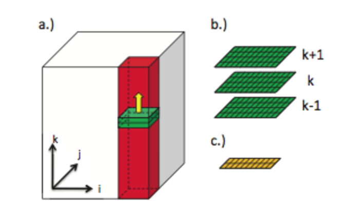
Figure 2: The “three planes” mechanism

Platform	number of threads	$T_{upd}$
Tesla C1060 GM	320	1.9 ns
Tesla C1060 CA	320	2.0 ns
Tesla C1060 SM	self determined	2.5 ns
Tesla C1060 SM4P	self determined	2.2 ns
Tesla C1060 TEXT	320	1.8 ns
GTX 480 (Fermi) GM	320	0.66 ns
GTX 480 (Fermi) CA	320	0.70 ns
GTX 480 (Fermi) SM	self determined	1.3 ns
GTX 480 (Fermi) SM4P	self determined	0.86 ns
GTX 480 (Fermi) TEXT	480	0.63 ns
Intel i7 (SSE instr.)	1	$\sim 13.5$ ns
Intel i7 (SSE instr. + OpenMP)	8	$\sim 5$ ns

Table 2: Timings for simulating a single Heisenberg spin glass system with continuous (gaussian distributed) isotropic couplings. The lattice size is set equal to $L=128$. $T_{upd}$ is the time in nanoseconds to process 1 spin. We ran 100 iterations and report the total time divided by the number of iterations and then divided by the number of spins in the system

The main results are reported in table 2. GM stands for Global GPU Memory. This is the most simple version which starts a very large number of threads and blocks by exploiting the fact that the Overrelaxation GPU kernel we wrote needs very few registers. The GPU kernel updates all white spins and then all black spins. The synchronization required between the updating of white and black spins is guaranteed by two distinct kernel invocations. To reduce the corresponding overhead, we could resort to a different synchronization mechanism although the lack of a native mechanism to synchronize, within a single kernel, the thread-blocks each other makes a bit tricky any alternative approach.

SM stands for Shared GPU Memory. This is the version which keeps three planes in shared memory and updates before white and then black spins of a plane before proceeding to the next plan. SM4P stands for Shared Memory version with 4 planes in memory. The difference with the SM version is that we update two plane concurrently (the white spins on the first plane and the black ones on the second plane and then the other way around: the black spins on the first plane and the white ones on the second plane). For the two shared memory versions (SM and SM4P) the number of threads is determined implicitly by the size of the available shared memory (so it varies between the Tesla C1060 where it is equal to 144 and the GTX 480 or the C2050 where it is equal to 384).

CA stands for “Cache”. This is the version developed for the Fermi architecture where a 48Kbyte cache is available on each MultiProcessor. The results in the table have been obtained by using the hint for L1 cache that sets it equal to 48K per MP. The idea is to update all the white spins of a plane and then all the black spins of the same plane. If the cache works as expected, three planes should be loaded when the white spins are updated. Then for the update of the black spins no new data should be loaded. We tested this version also on the Tesla architecture, although the Tesla does not have a cache, just to measure the overhead introduced by processing a single plane in each kernel.
Finally, we measured the overhead of invoking a CUDA kernel. This is basically independent on the method and represents a lower bound of the time that the update of a spin requires. The value we found is $0.1$ ns per spin.

Number of hits	$T_{upd}$ sm_arch=20	$T_{upd}$ sm_arch=13
1	0.911 ns	0.856 ns
2	0.606 ns	0.546 ns
5	0.429 ns	0.366 ns
10	0.373 ns	0.311 ns
$\infty$ (extrapolated)	0.313 ns	0.246 ns

Table 3: Timings with respect to the number of hits for the SM4P version on a GTX 480. Timings are reported for the compilation with two different setups (arch=sm_20, corresponding to the latest generation software that works only on the Fermi architecture and arch=sm_13 that works for both the previous and the latest architecture). The test case is the same as in table 2.

Platform	$T_{upd}$ ECC on	$T_{upd}$ ECC off
C2050 (Fermi) GM	1.0 ns	0.84 ns
C2050 (Fermi) CA	1.1 ns	0.87 ns
C2050 (Fermi) SM	1.63 ns	1.66 ns
C2050 (Fermi) SM4P	1.4 ns	1.3 ns
C2050 (Fermi) TEXT	1.0 ns	0.78 ns

Table 4: Timings with and without Error Checking and Correction on a C2050 (the GTX 480 does not have ECC). The test case is the same as in table 2. The compilation setup is arch=sm_13.

5 Discussion and Conclusions

In table 3 we report the results of a test in which the spins of the version SM4P are updated multiple times (“multi hit”) before moving to the next two planes. Since the updates after the first one do not require new accesses to the global memory (all data are already in the shared memory) this technique allows to measure the overhead introduced by the initial loading of the data as the difference between the total time required by the single hit and the time required by an infinite number of hits. Obviously it is not possible to carry out an infinite number of hits but it is easy to extrapolate the corresponding value by using a simple fit. The time we found is $\sim 0.6$ ns for both the compilation setups used for the tests. Interestingly, at this time, it is more efficient to compile on the Fermi architecture with a setup (arch=sm_13) introduced for the previous generation GPUs. On the other hand it is absolutely necessary to take into account the specific features of the new architecture like the different size of the shared memory or the new integer multiplication capability. For instance, if on the Fermi architecture the multiplication between two integers is carried out by using the __mul24 (as it was suggested on the previous generation GPUs when the result of the multiplication fitted in 24 bits) there is a penalty of about $5\%$ for our code. If we consider the time ($0.63$ ns per spin update) required by the best “single-hit” technique, that is the texture based one, and use the estimate of 60 floating point operations per spin update (that does not take into account the index arithmetics), we obtain a sustained performance very close to $100$ GFlops. Besides that, the most interesting observation is that, despite the much higher latency of the global memory, the simple versions (the GM one and the TEXT one) that use neither the shared memory nor the cache (where available) are significantly faster unless a “multi-hit” variant of the shared memory version is used. A possible explanation of this behaviour is that the limited size of the shared memory (and of the cache) allows to start fewer threads with respect to the case of a global memory based version where the only limitation is the number of registers. Moreover, although the shared memory version allows to reduce the number of global memory transactions when loading data (spins and couplings), it offers no advantage when the updated spins are stored back in global memory. The advantage of using texture fetches instead of simple load operations from the global memory is quite limited (about $5\%$). However, only very minor changes are required to the code to take this advantage so it is worth it. It is more puzzling that, apparently the cache does not offer advantages at all. A possible explanation is that the overhead introduced by calling the computational kernel a number of times equal to twice the linear dimension of the lattice (instead of calling it just once as we do in the GM or TEXT version) is as large and possibly larger than the saving in time that the cache may offer. The requirement of calling the kernel multiple times arises because on each plane it is necessary to update all white spins and then all black spins. So, for each step in the $Z$ direction, two invocations are required.
As shown in table 4, the Error Checking and Correction introduces a sizeable overhead for the methods working in global memory (GM, TEXT, CA). For reasons that we could not determine, the methods working in shared memory undergo a much more limited penalty when the ECC is on.
Finally, it is worth to highlight two facts: i) a well tuned GPU implementation can achieve almost an order of magnitude of speedup with respect to a well tuned vector-multicore implementation ($0.63$ ns per spin update for the TEXT version on the GTX 480 vs. $5$ ns per spin update on a multicore Intel i7; ii) the performances of the GPUs keep on to increase significantly in a pretty short time (the performances of the new architecture are double and in some cases even more than double with respect to the previous generation cards that are only two years old) making it a very interesting platform for the numerical simulation of spin systems.

References

- [1] NVIDIA CUDA Compute Unified Device Architecture Programming Guide http://www.nvidia.com/cuda
- [2] Preism T, Virnau P, Paul W, and Schneider JJ, GPU accelerated Monte Carlo simulation of the 2D and 3D Ising model. Journal of Computational Physics 228, 4468-4477 (2009).
- [3] Sanz González J M, Heisenberg spin glass on graphic cards: preliminary tests (in preparation).
- [4] Adler S, Over-relaxation method for the Monte Carlo evaluation of the partition function for multiquadratic actions. Phys. Rev. D 23, 2901–2904 (1981).
-
[5]
Hower L, Thomas D,
Efficient Random Number Generation and Application Using CUDA,
http://http.developer.nvidia.com/GPUGems3/gpugems3_ch37.html - [6] Landau D, Vectorisation of Monte Carlo programs for lattice models using supercomputers, in “The Monte Carlo Method in Condensed Matter Physics”, Topics in Applied Physics, Volume 71 (1992).
-
[7]
Giles M, Jacobi iteration for a Laplace discretisation
on a 3D structured grid
http://people.maths.ox.ac.uk/ gilesm/codes/laplace3d/laplace3d.pdf -
[8]
Fatica M, Phillips E H, Implementing the Himeno
Benchmark with CUDA on GPU clusters,
http://www.citeulike.org/user/naoya/article/7163266(2009).