Models of population dynamics under the influence of external perturbations: mathematical results

Abstract.

In this Note, we describe the stationary equilibria and the asymptotic behaviour of an heterogeneous logistic reaction-diffusion equation under the influence of autonomous or time-periodic forcing terms. We show that the study of the asymptotic behaviour in the time-periodic forcing case can be reduced to the autonomous one, the last one being described in function of the “size” of the external perturbation. Our results can be interpreted in terms of maximal sustainable yields from populations. We briefly discuss this last aspect through a numerical computation.

Résumé: Analyse de modèles de dynamique de populations sous l’influence de perturbations externes. Cette Note a pour objet l’étude des états stationnaires et du comportement asymptotique d’équations de réaction-diffusion avec coefficients hétérogènes en espace, auxquelles nous ajoutons un terme de perturbation stationnaire ou périodique en temps. Nos résultats peuvent s’interpreter en termes de récolte maximale supportable par une population. Nous soulignons cet aspect à l’aide d’un calcul numérique.

1. Introduction

The purpose of this Note is to study the following model:

(1.1) $$u_{t}=\nabla\cdot(A(x)\nabla u)+u(\mu(x)-\nu(x)u)-f(\omega t,x)\rho_{\varepsilon}(u),\ (t,x)\ \in\ \mathbb{R}_{+}\times\Omega.$$

The reaction-diffusion models of the type $u_{t}=\nabla\cdot(A(x)\nabla u)+u(\mu(x)-\nu(x)u)$ correspond to the natural extension of the classical Fisher model [4]. They were first introduced by Shigesada et al. [9] for population dynamics. Our aim is to understand the asymptotic behaviour of the solutions of such models, when we add a time-periodic forcing term $f(\omega t,x)$. With such additional term, this can interpreted as an harvesting model with seasonal harvesting. In real-life context this perturbation term can arise when a quota is set on the harvesters.

We make the following assumptions on the coefficients: the diffusion matrix $A(x)$ is assumed to be of class $C^{1,\alpha}$ (with $\alpha>0$) and uniformly elliptic; i.e. there exists $\tau>0$ such that $A(x)\geq\tau I_{N}$ for all $x\in\Omega$. The functions $\mu$ and $\nu$ belong to $L^{\infty}(\Omega)$. Moreover, we assume that there exist $\underline{\nu}$ and $\overline{\nu}$ such that $0<\underline{\nu}<\nu(x)<\overline{\nu}$ for all $x$ in $\Omega$. The function $f$ is 1-periodic in the first variable and belongs to $C^{0}(\mathbb{R}\times\Omega)$, and the function $\rho_{\varepsilon}$ defines a “regularized threshold”: it is a $C^{1}(\mathbb{R})$ nondecreasing function such that $\rho_{\varepsilon}(s)=0$ for all $s\leq 0$ and $\rho_{\varepsilon}(s)=1$ for all $s\geq\varepsilon$. This threshold guarantees the non-negativity of the solutions of (1.1).

Two kinds of domains $\Omega$ are considered: either $\Omega=\mathbb{R}^{N}$ or $\Omega$ is a smooth bounded domain of $\mathbb{R}^{N}$. We qualify the first case, $\Omega=\mathbb{R}^{N}$, as the sp-case and the second one as the bounded case. Indeed, in the sp-case, we assume that $A(x)$, $\mu(x)$, $\nu(x)$ and $f(s,x)$ depend on the variables $x=(x_{1},\cdots,x_{N})$ in a space-periodic fashion (i.e. for $L_{1},\ldots,L_{N}$ fixed positive numbers, a function $g$ is said to be sp-periodic if $g(x+k)=g(x)$ for all $x\in\mathbb{R}^{N}$ and $k\in L_{1}\mathbb{Z}\times\cdots\times L_{N}\mathbb{Z}$). In the bounded case, throughout this paper, we assume that we have Neumann boundary conditions on $\partial\Omega$.

2. The case of autonomous forcing

All the results of this section remain true either in the sp-periodic or bounded cases. The proofs are detailed in [7].

We consider the equation (1.1) with $f(wt,x)=\delta h(x)$, i.e.

(2.1) $$u_{t}=\nabla\cdot(A(x)\nabla u)+u(\mu(x)-\nu(x)u)-\delta h(x)\rho_{\varepsilon}(u),\ (t,x)\ \in\ \mathbb{R}_{+}\times\Omega,$$

where $h$ is a continuous function such that there exist $\alpha,\beta>0$ with $\alpha<h(x)<\beta\hbox{ for all }x\in\Omega$, and which is sp-periodic in the sp-case.

Let $\lambda_{1}$ be defined as the unique real number such that there exists a function $\phi>0$ which satisfies

(2.2) $$-\nabla\cdot(A(x)\nabla\phi)-\mu(x)\phi=\lambda_{1}\phi\hbox{ in }\Omega,\phi>0\hbox{ and }\|\phi\|_{\infty}=1,$$

with either periodic or Neumann boundary conditions, depending on $\Omega$, as mentioned above. The function $\phi$ is uniquely defined by (2.2) (the existence and uniqueness of $\lambda_{1}$ and $\phi$ follow from the standard Krein-Rutman theory).

Remark 2.1.

Note that if we assume that $\lambda_{1}<0$ and $\delta=0$, then, given any continuous and bounded function $u_{0}$, the solution $u(t,x)$ of (2.1) with initial data $u_{0}$ converges to a function $p$ which is the unique bounded and positive solution of $\nabla\cdot(A(x)\nabla p)+p(\mu(x)-\nu(x)p)=0$, $x\in\Omega$. These convergence, as well as existence and uniqueness results are proved in [2].

We first describe the steady states of (2.1) without “regularized threshold”:

(2.3) $$\nabla\cdot(A(x)\nabla p_{\delta})+p_{\delta}(\mu(x)-\nu(x)p_{\delta})-\delta h(x)=0,\ x\ \in\ \Omega.$$

Using a Leray-Schauder degree argument, together with the uniqueness of the solution $p$ defined in the above remark, we prove the following

Theorem 2.1.

There exists $\delta^{*}>0$ such that for all $\delta$ s. t. $0<\delta<\delta^{*}$, (2.3) admits two distinct positive solutions, $p^{1}_{\delta}$ and $p^{2}_{\delta}$. Moreover, $p^{1}_{\delta}\to 0$ and $p^{2}_{\delta}\to p$ uniformly in $\Omega$ as $\delta\to 0$.

Let us set $\displaystyle{\underline{\phi}:=\min_{x\in\Omega}\phi(x)},$ $\delta_{1}:=\displaystyle{\frac{\lambda_{1}^{2}\underline{\phi}}{\beta\overline{\nu}(1+\underline{\phi})^{2}}}$ and $\delta_{2}:=\displaystyle{\frac{\lambda_{1}^{2}}{4\alpha\underline{\nu}}}.$ Then we have the following theorem:

Theorem 2.2.

- (i) If $\lambda_{1}<0$ and $\delta\leq\delta_{1}$, then there exists a positive bounded solution $p_{\delta}$ of (2.3) such that $p_{\delta}\geq\displaystyle{-\frac{\lambda_{1}\phi}{\overline{\nu}(1+\underline{\phi})}}$ (in particular $\max p_{\delta}\geq\frac{-\lambda_{1}}{2\overline{\nu}}$).

(ii) If $\lambda_{1}<0$ and $\delta>\delta_{2}$, or if $\lambda_{1}\geq 0$, there is no positive bounded solution of (2.3).

The proof relies on monotone methods of sub- and super-solutions. For the existence result (i), we have computed a sub-solution of the form $\kappa\phi$ with $\kappa>0$. The optimal value of $\kappa$, in the sense that it gives the highest value of $\delta_{1}$, is $\kappa_{0}=\displaystyle{-\lambda_{1}/(\overline{\nu}+\overline{\nu}\underline{\phi})}$. We have numerically computed the values of $\delta_{1}$ and $\delta_{2}$ in several particular examples of sp-case (see Figure 1). The results illustrate the effect of environmental fragmentation on the maximum sustainable yield, and show that the interval $(\delta_{1},\delta_{2}]$ on which we have no theoretical information can be very narrow (see Figure 1-(c)).

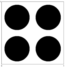
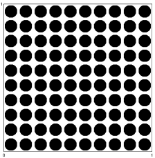
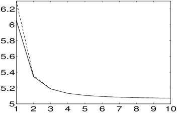
Figure 1. $N=2$, $A=I_{2}$, $\nu\equiv 1$, $h\equiv 1$ and $\mu(x)$ is $(1,1)$-periodic and takes two values, $\mu\equiv-1$ on $\Omega_{-}$ and $\mu\equiv 10$ on $\Omega^{+}$, where $\Omega^{+}$ consists on $k^{2}$ equally-spaced disks such that, on each period cell $[0,1]^{2}$, $|\Omega^{+}\cap[0,1]^{2}|=1/2$, and $\Omega^{-}=\mathbb{R}^{2}\backslash\Omega^{+}$. (a) A period cell with $k=2$ (b) $k=10$; $\Omega^{+}$ is represented in black. (c) The values of $\delta_{1}$ (continuous line) and $\delta_{2}$ (dashed line) in function of $k$.

Let us turn to the study of the evolution equation (2.1). We assume that $\lambda_{1}<0$ and $\varepsilon$ is such that $\displaystyle{\varepsilon_{0}:=2\frac{\varepsilon\overline{\nu}}{\underline{\phi}}}<\displaystyle{\frac{-\lambda_{1}}{2}}$; we prove the following theorem:

Theorem 2.3.

Let $u(t,x)$ be the solution of (2.1) with initial data $u(0,x)=p(x)$ defined in Remark 2.1. Then $u$ is non-increasing in $t$ and we have the following asymptotic behaviour

(i) if $\delta\leq\delta_{1}$, $u(t,x)\to p_{\delta}(x)$ uniformly in $\Omega$ as $t\to+\infty$, where $p_{\delta}$ is the unique positive maximal solution of (2.3); and

(ii) if $\delta>\delta_{2}$, then $u(t,x)<\varepsilon_{0}$ for $t$ large enough.

In the above theorem, we assume that $u(0,x)=p(x).$ This means that harvesting starts on a stabilized population governed by the standard Fisher model without external forcing.

Remark 2.2.

These results are sharper than those which could be obtained by a standard La Salle invariance principle, since we obtain here discriminatory bounds on $\delta$, which determine the asymptotic behaviour of the solutions.

3. Time-periodic forcing

In this section we consider the general equation (1.1) in the bounded case, with $\omega>0$ defined as the frequency of the forcing term. All the results are proved in [3]. Let us introduce $T:=\omega^{-1}$. It is known that under the above assumptions on $A(x)$, $\mathcal{A}u=-\nabla\cdot(A(x)\nabla u)$ is a sectorial operator with domain $\mathcal{D}(\mathcal{A})=\{u\in H^{2}(\Omega),\mbox{ s. t. }\partial_{n}u=0\ \mbox{ on }\partial\Omega\}$ (see e.g. [6]). As a consequence, $-\mathcal{A}$ generates an analytic semigroup $e^{-\mathcal{A}t}$ on $L^{2}(\Omega)$. Let $\{V^{2r}\}_{\{r\geq 0\}}$ be the family of interpolation spaces generated by the fractional powers of $\mathcal{A}$, where $V^{2r}=\mathcal{D}(\mathcal{A}^{r})$ (see [8] for details). The existence of a $T$-periodic solution of the equation (1.1) can be reached by several procedures (e.g. averaging method [5]). We present here a result on the existence of a hyperbolic $T$-periodic solution, which is related to the robustness of a hyperbolic stationary solution of the autonomous equation (2.1), with $\delta h(x)=\int_{0}^{1}f(s,x)ds$. More precisely,

Theorem 3.1.

Assume that equation (2.1) has a hyperbolic stationary solution $q\in V^{2r}$, $0\leq r\leq 1$. Then there exists $\omega^{*}>0$ such that for every $\omega\geq\omega^{*}$, the problem (1.1) possesses a hyperbolic $T$-periodic solution $u_{\omega}(t)$ such that for any $t\in[0,T]$, $u_{\omega}(t)$ lives in a $V^{2r}$-neighborhood of $q$. Furthermore if $\omega\rightarrow+\infty$, then $u_{\omega}(t)\rightarrow q$ in $V^{2r}$.

The proof uses similar arguments as the one of [8] Theorem 76.1, and is therefore based on a Lyapunov-Perron type argument; the existence of such a hyperbolic periodic orbit is achieved via a fixed point argument on the following operator:

$$\xi\rightarrow\mathcal{T}(f)\xi:=\int_{-\infty}^{t}Qe^{-L(t-s)}(E(q,\xi)+f(ws,\cdot))ds...$$

$$...-\int_{t}^{+\infty}Pe^{-L(t-s)}(E(q,\xi)+f(ws,\cdot))ds,$$

where $L=\mathcal{A}-(\mu(x)-2\nu(x)q)\mathcal{I}$, $E(q,\xi)=-2\nu(x)\xi^{2}$, $\xi$ belongs to a subset of $L^{\infty}(\mathbb{R},V^{2r})\cap C^{0}(\mathbb{R},V^{2r})$, and $P$ and $Q$ are the associated projectors with the exponential dichotomy for equation (2.1) related to the existence of a hyperbolic stationary solution.

The main interest of Theorem 3.1 is that it gives a simple sufficient condition to ensure the existence of a $T$-periodic solution of (1.1) and that it allows to localize in physical space where this solution can appear. Another interesting aspect of this theorem is that it reduces the study of existence and stability of a $T$-periodic solution of (1.1) to that of the hyperbolic equilibria of the autonomous version (2.1). For instance we get as an application of Theorems 2 and 4 for $\lambda_{1}<0$ and $f(wt,x)=\delta g(wt,x)$ with $\alpha<\int_{0}^{1}g(s,x)ds<\beta$ for all $x\in\Omega$, that if $\delta\leq\delta_{1}$ and $\omega$ sufficiently large, then there exists a stable non-trivial $T$-periodic solution $u_{\omega,\delta}$ of $(\ref{eq_evo})$ in a neighborhood of a solution $p_{\delta}$ of (2.3).

Note added for this version on ArXiV: The reference [7] cited here, corresponds the article of the authors entitled “On Population Resilience to External Perturbations” which has been published in SIAM J. Appl. math (SIAP), 68 (1), (2007) 133 -153. We kept here the old reference [7] as in the original article published in C. R. Acad. Sci. Paris, Ser. I, 343: 307-310; before the SIAP article. The reference [3] below is still under preparation.

References

- [1]
- [2] H. Berestycki, F. Hamel, L. Roques. Analysis of the periodically fragmented environment model : I - Species persistence. J. Math. Biol. 51 (1) (2005) 75-113.
- [3] M. Chekroun, L. Roques, Spatialized harvesting models. The influence of seasonal variations, in preparation.
- [4] R.A. Fisher, The advance of advantageous genes, Ann. Eugenics 7 (1937) 335-369.
- [5] J.K. Hale, S.M. Verduyn Lunel, Averaging in Infinite Dimensions, Journal of Int. Eq. and Appl. 2 (4) (1990) 463-494.
- [6] A. Pazy, Semigroup of Linear Operators and Applications to Partial Differential Equations, Springer-Verlag, 1983.
- [7] L. Roques, M. Chekroun, Harvesting models in heterogeneous environments, Preprint (2006).
- [8] G.R. Sell, Y. You, Dynamics of Evolutionary Equations, Springer-Verlag, 2002.
- [9] N. Shigesada, K. Kawasaki, E. Teramoto, Traveling periodic waves in heterogeneous environments, Theor. Population Biol. 30 (1986) 143-160.
- [10]