A 33 GHz VSA survey of the Galactic plane from $\ell=27^{\circ}$ to $46^{\circ}$

Abstract

The Very Small Array (VSA) has been used to survey the $\ell\sim 27^{\circ}$ to $\sim 46^{\circ}$, $|{\it{b}}|<4^{\circ}$ region of the Galactic plane at a resolution of 13 arcmin. This $\ell$-range covers a section through the Local, Sagittarius and the Cetus spiral arms. The survey consists of 44 pointings of the VSA, each with a r.m.s. sensitivity of $\sim 90$ mJy beam^-1. These data are combined in a mosaic to produce a map of the area. The majority of the sources within the map are HII regions.

The main aim of the programme was to investigate the anomalous radio emission from the warm dust in individual HII regions of the survey. This programme required making a spectrum extending from GHz frequencies to the FIR IRAS frequencies for each of 9 strong sources selected to lie in unconfused areas. It was necessary to process each of the frequency maps with the same u,v coverage as was used for the VSA 33 GHz observations. The additional radio data were at 1.4, 2.7, 4.85, 8.35, 10.55, 14.35 and 94 GHz in addition to the 100, 60, 25 and 12 $\mu$m IRAS bands. From each spectrum the free-free, thermal dust and anomalous dust emission were determined for each HII region. The mean ratio of 33 GHz anomalous flux density to FIR 100 $\mu$m flux density for the 9 selected HII regions was $\Delta S(33~{}{\rm GHz})/S(100~{}\mu$m$)=1.10\pm 0.21\times 10^{-4}$. When combined with 6 HII regions previously observed with the VSA and the CBI, the anomalous emission from warm dust in HII regions is detected with a 33 GHz emissivity of $4.65\pm 0.40$ $\mu$K (MJy/sr)^-1 ($11.5\sigma$). This level of anomalous emission is 0.3 to 0.5 of that detected in cool dust clouds.

A radio spectrum of the HII region anomalous emission covering GHz frequencies is constructed. It has the shape expected for spinning dust comprised of very small grains. The anomalous radio emission in HII regions is on average $41\pm 10$ per cent of the radio continuum at 33 GHz. Another result is that the excess (i.e. non-free-free) emission from HII regions at 94 GHz correlates strongly with the 100 $\mu$m emission; it is also inversely correlated with the dust temperature. Both these latter results are as expected for very large grain dust emission. The anomalous emission on the other hand is expected to originate in very small spinning grains and correlates more closely with the 25 $\mu$m emission.

1 INTRODUCTION

Radio surveys of the Galactic plane show the presence of small diameter sources embedded in a diffuse background. These sources have been identified as supernova remnants (SNRs) and HII regions, with an occasional extragalactic source. Each has a characteristic flux density spectral index $\alpha$ defined as $S\sim\nu^{\alpha}$; for SNRs $\alpha$ is in the range $-$0.3 to $-$0.8 with an average of $-$0.5 at GHz frequencies (Green 2009), while for HII regions $\alpha$ is restricted to the range -0.11 to -0.13 (Dickinson, Davies & Davis 2003) depending on frequency and electron temperature. The diffuse emission centred about the Galactic plane has conventionally been interpreted as a mix of synchrotron emission with $\alpha\sim-0.7$ at $\nu<1$ GHz and free-free emission. Synchrotron dominates at $\nu<1$ GHz.

In the last 10 years this picture has changed radically following the identification of a third emission component which is strongly correlated with interstellar dust as mapped at FIR wavelengths by IRAS for example. This component was first identified in the early searches for fluctuations in the Cosmic Microwave Background (CMB) at frequencies in the range 10 to 60 GHz (Leitch et al. 1997; de Oliveira-Costa et al., 1999, 2002, 2004; Kogut et al. 1996) when it was variously interpreted as emission from very hot or from normal interstellar ionized gas which was correlated with FIR dust emission. The situation became clearer when all-sky radio and H$\alpha$ surveys became available along with an emission model for spinning dust (Draine & Lazarian 1998) to complement the all-sky multi-frequency survey by COBE and later by WMAP. The three components could then be separated and evaluated (Banday et al. 2003, Lagache 2003; Davies et al. 2006; Miville-Deschênes & Lagache 2005).

The definitive determinations of the spectrum of spinning dust have come from the observations of compact dust clouds both at intermediate latitudes and near the Galactic plane. The best examples are the Perseus molecular cloud (Watson et al. 2005, Tibbs et al. 2010) and the Lynds dark nebula LDN1622 (Finkbeiner et al. 2002, 2004; Casassus et al. 2006). Additional detections in dark clouds have recently been reported (Scaife et al. 2009). The peak in the emission is in the range 20 to 30 GHz and is at a level compatible with the Draine & Lazarian theory.

Many of the dust clouds studied are in star-forming regions which include HII regions; the additional free-free emission complicates the situation; this problem can be resolved by using data from a range of radio frequencies to separate the emission components. Nonetheless, tentative detections of anomalous emission have been made in some bright HII regions (Dickinson et al. 2007, 2009) while no detections or upper limits have been made in others (Dickinson et al. 2006; Scaife et al. 2008). The present 33 GHz survey of a rich $19^{\circ}\times 6^{\circ}$ area of the northern Galactic plane is aimed at significantly improving knowledge of anomalous emission from bright HII regions and at the same time identifying the detected sources as HII regions, SNRs or extragalactic objects. Anomalous emission from HII regions is predicted by spinning dust models (Draine & Lazarian 1998, Ali-Haïmoud et al. 2009).

The paper is organized as follows. Section 2 gives a summary of the parameters of the Very Small Array (VSA) when operated in its extended configuration. Section 3 describes the calibration and data reduction methods. The procedure for producing the maps, including the mosaicing technique as applied to both the VSA 33 GHz data and the ancillary data, is given in Section 4. In Section 5 we describe the method of extracting flux densities and dimensions of the brightest sources. Section 6 describes the astronomical results of the survey which include a clear determination of the spectrum of spinning dust in HII regions and a description of the physical conditions in the warm dust associated with the detected HII regions. Section 7 discusses the properties of the excess emission while Section 8 discusses other properties of the HII regions. Conclusions are given in Section 9.

2 THE VSA EXTENDED ARRAY

The VSA is an interferometer situated at the high and dry site of the El Teide Observatory, Tenerife, at an altitude of 2340 m. The array operates in the $\it{Ka}$ band (26-36 GHz); the observations for this Galactic plane survey were made at a centre frequency of 33 GHz and a bandwidth of $\Delta\nu\sim$ 1.5 GHz. The 14 horns of the array are mounted on a $4\times 3$ m² tip-tilt table, inside a metal screen which minimizes ground spillover. In the extended mode of the VSA each corrugated horn feeds a 322 mm aperture mirror; the baselines available are in the range 0.6 to 2.5 m. Each horn feed has a primary beamwidth of FWHM $2^{\circ}.12$ at 33 GHz. The effective resolution of the extended array is approximately 13 arcmin (uniform weighting) at 33 GHz. The geometry of the tip-tilt table and the screen restrict observations to elevations above $\sim 55^{\circ}$; the corresponding declination range is $-5^{\circ}$ to $+65^{\circ}$.

The point source sensitivity of the extended VSA is $\sim 6$ Jy s^1/2 at an average system temperature of 35 K. The corresponding brightness temperature sensitivity is $\sim 15$ mK s^1/2 in the synthesized beam area of $\sim 1.4\times 10^{-5}$ sr. Unlike the Cosmic Background Imager (CBI), which used a co-mounted array, the VSA does not require the subtraction of a lead/trail reference field. This is because the tracking VSA antennas provide a non-zero astronomical fringe rate.

Table 1: VSA specs.

Description	phase-switching interferometer
Location	Izaña, Tenerife
Altitude	2340 m
Number of antennas (baselines)	14 (91)
Baseline lengths	0.6 m - 2.5 m
Centre frequency	33 GHz
Bandwidth, $\Delta\nu$	1.5 GHz
Correlator	91 channel complex correlator
Mirror size	322 mm
Primary beam (FWHM)	$2^{\circ}.12$
Synthesized beam (FWHM)	$\sim 13^{\prime}$
System temperature, $T_{sys}$	$\sim 35$ K
Point-source flux sensitivity	$\sim 6$ Jy s1/2
Temperature sensitivity	$\sim 15$ mK s1/2

Table 1 summarizes the specification of the extended VSA. Further details of the technical specifications of the VSA may be found in Watson et al. (2003), Scott et al. (2003) and Maisinger et al. (2003).

3 OBSERVATIONS AND DATA REDUCTION

3.1 Observations

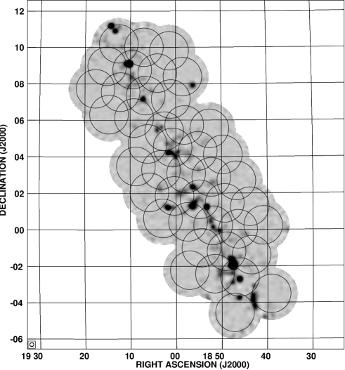
Figure 1: The solid circles show the pointing positions for the 44 VSA fields superposed on the 33-GHz VSA mosaic. The size of the circles is the FWHM primary beam of the VSA in extended mode.

The 33-GHz Galactic plane survey was made between July 2002 and August 2003, when the VSA was in the extended configuration. Fig. 1 shows the area of the Galactic plane covered which extends northwards from the southern limit of the VSA (Dec $=-5^{\circ}$). The circles show half-power beamwidths of the 44 fields observed. The outer envelope of the survey represents the $\frac{1}{4}$-power level of the survey; a map can be reliably reconstructed within this 114 deg² area. The overlap of the fields ensures that more than one independent observation is made of each source in the survey area. Three fields are missing for complete coverage of the area (G332$-$226, G396$-$226, G396$+$226).

On any day the VSA observed one field for typically $\sim 2.4$ hours. Some of the low declination fields were observed more than once. Calibrator observations of nearby bright radio sources were interleaved with the field observations. These were typically observed for a minimum of 10 minutes. The properties of the calibrators are discussed in detail in Sections 3.3 and  3.4.

The 44 pointings are listed in Table 2. Note that the actual integration time is typically $\sim 80$ per cent of the values indicated in the table, due to data editing and atmospheric effects, as discussed in the following section.

Table 2: The Galactic coordinates of the centres of fields observed with the extended VSA. Column 4 lists the integration time for each field.

Field	$\ell$	b	$t_{\rm int}$ (hrs)
G284-113	28.4	-1.13	5.03
G284+113	28.4	+1.13	2.43
G300+000	30.0	0.00	7.53
G308-113	30.8	-1.13	7.39
G308+113	30.8	+1.13	2.46
G316+000	31.6	0.00	2.46
G316-226	31.6	-2.26	3.21
G316+226	31.6	+2.26	2.45
G324-113	32.4	-1.13	2.28
G324+113	32.4	+1.13	2.46
G332+000	33.2	0.00	2.31
G332-226	33.2	-2.26	2.30
G332+226	33.2	+2.26	2.18
G340-113	34.0	-1.13	2.41
G340+113	34.0	+1.13	2.32
G348+000	34.8	0.00	2.32
G348-226	34.8	-2.26	2.47
G348+226	34.8	+2.26	2.31
G356-113	35.6	-1.13	2.41
G356+113	35.6	+1.13	2.42
G364+000	36.4	0.00	2.40
G364-226	36.4	-2.26	2.39
G364+226	36.4	+2.26	2.32
G372-113	37.2	-1.13	2.32
G372+113	37.2	+1.13	2.34
G380+000	38.0	0.00	2.31
G380-226	38.0	-2.26	2.31
G380+226	38.0	+2.26	2.34
G388-113	38.8	-1.13	2.29
G388+113	38.8	+1.13	2.31
G396+000	39.6	0.00	2.45
G404-113	40.4	-1.13	2.21
G404+113	40.4	+1.13	2.25
G412+000	41.2	0.00	2.37
G412-226	41.2	-2.26	2.42
G412+226	41.2	+2.26	2.43
G420-113	42.0	-1.13	2.51
G420+113	42.0	+1.13	2.31
G428+000	42.8	0.00	2.38
G428-226	42.8	-2.26	2.37
G428+226	42.8	+2.26	2.38
G436-113	43.6	-1.13	2.37
G436+113	43.6	+1.13	2.34
G444+000	44.4	0.00	2.35

3.2 Data reduction pipeline

The data reduction and calibration of all the 44 fields were made with the REDUCE package which was written specifically for the VSA (e.g. Dickinson et al. 2004). Every field was analyzed separately. The data for each field were first checked for atmospheric, pointing and geometry errors; data lying outside the allowed parameter range were automatically flagged. Gain and phase corrections based on the calibration observations were then implemented.

Fourier filtering was used to remove correlated signals due to ground effects and the Sun or Moon if nearby (Watson et al., 2003). This filtering process has no effect on the data because of the difference in fringe rates between the astronomical and non-astronomical signals. Data were filtered if the Sun and the Moon were within 27^∘ and 18^∘ of the field centres, respectively. Observations were not used if the Sun or the Moon were within 9^∘ of the field centre. The final step in the reduction pipeline was to take account of the apparent noise levels in the 91 baselines arising from the different receiver temperatures and bandwidths; the measured r.m.s. noise on each baseline was used to reweight the data to give optimal sensitivity.

3.3 The daily amplitude and phase measurement

The daily observation of the Galactic plane was interleaved with observations of calibration sources whose positions and flux densities were known. These observations were used to calibrate the survey data in amplitude and phase. The phases of each of the 91 baselines could be estimated to better than $\sim 10^{\circ}$. The overall system noise was continuously compared using noise signals injected into each of the 14 feed horns; variations in the system noise in each receiver due to changing atmospheric emission were used to correct the astronomical amplitudes. These corrections were typically less than a few percent. Any data with a correction factor of more than $10$ per cent were discarded.

3.4 Absolute flux calibration

The flux densities and the brightness temperatures used here are the 33 GHz values determined at epoch 2001 from VSA measurements in the period 2001 - 2004 (Hafez et al, 2008). The “absolute” calibration was made in terms of the brightness temperature of the planet Jupiter given by the WMAP 5-year data (Hill et al. 2009), namely $T_{b}=146.6\pm 0.75$ K. $T_{b}$ values for the planets were converted to flux densities using the Ephemeris values of the planet areas. The radio sources Cas A and Tau A are sufficiently extended ($\sim 5$-arcmin diameter) that corrections were required to the data, as given by Hafez et al. (2008). Over this period the sources Cas A, Tau A and NGC7027 were decreasing by several tenths of 1 percent per annum at 33 GHz.

The flux density scale provided by the calibrators is believed to be better than $2$ per cent; it is tied to the Jupiter brightness temperature as described above.

4 IMAGING AND MOSAICING THE 33-GHz DATA

We describe here the main steps in imaging the individual VSA fields and then combining them into a mosaic of the Galactic plane field.

4.1 The individual VSA fields

Each of the fields was imaged by applying the DIFMAP package (Shepherd, 1997) to the visibility data, using uniform weighting to give optimal resolution and retain extended emission. The CLEAN algorithm (Högbom, 1974) was applied to the dirty images; typically 5000 iterations with a low gain loop of 0.01 were used. The resultant r.m.s. noise on a typical field with a 2 hour integration was $\sim 90$ mJy beam^-1. This corresponds to 7.5 Jy beam^-1 $s^{1/2}$ which is close to the noise expected from $T_{sys}$ and the 1.5 GHz bandwidth (Table 1).

4.2 Mosaicing - the final map

The individual field images were combined into a map using the HGEOM and LTESS tasks of the $\mathcal{AIPS}$ package. The LTESS task also corrects the individual field maps for the $2^{\circ}.1$ FWHM primary beam response and restricts the field to the $25$ per cent beam level. The half-power and quarter-power levels are shown in Fig. 1.

The final map which combines the 44 fields is shown in Fig. 2, plotted in Galactic coordinates. The region covered is $\ell=27^{\circ}$ to $46^{\circ}$ and ${b}=-3^{\circ}\!.5$ to $+3.5^{\circ}$. The areas around the edge of the map have higher noise level due to the correction for beam taper.

4.3 The noise level on the 33-GHz map

The noise on the mosaiced map was estimated from the higher latitude parts of the field which were free of obvious sources. The effective integration time over the map is $\sim 2$ hours when account is taken of overlapping fields and of the $\sim 20$ per cent data loss due to weather, ground effects on short baselines and equipment malfunction. The calculated average r.m.s. noise was 94 mJy beam^-1. This value is as expected from the single field measurements.

Effective noise levels are however greater near the Galactic plane where there are strong sources as well as a diffuse background, $\sim 2^{\circ}$ wide in latitude. Here the noise level may amount to $\pm 1$ per cent of the adjacent source due to either limited coverage of the $\it{u,v}$ plane or flux leakage from incorrect phase calibration.

5 Derivation of source parameters

We outline here the procedures applied to derive the source parameters - flux density, position and angular size - detected in the survey.

5.1 Applying JMFIT

The task JMFIT in $\mathcal{AIPS}$ was used to determine the parameters of the strongest and most clearly defined sources in the survey area. JMFIT finds the best elliptical Gaussian fit plus a baseline offset to a source and gives the peak flux density, the integrated flux density, the position coordinates, angular size and position angle, each with an associated error.

Where the source is complex, JMFIT can in principle fit several components; with the S/N available in the present survey we restricted the fit to 2 Gaussian components for the brightest objects. A test of the uncertainty of the source parameters was to make solutions with different box sizes which allowed a range of base levels to be applied.

5.2 Confirmation with IRING

The $\mathcal{AIPS}$ task IRING was used to confirm the results obtained with JMFIT, particularly where a Gaussian assumption was inappropriate in more complex sources. IRING requires the specification of the source centre and integrates the flux density in successive rings around this centre.

This procedure enables integrated flux densities to be estimated out to specified background levels.

The derived values of integrated flux density in most cases agreed to better than $5-10$ per cent with the values determined from JMFIT. Since the IRING task does not give angular size or position information, the JMFIT data are used for these parameters.

5.3 Accuracy of the 33-GHz data

As shown in Section 4.3 the r.m.s. noise on individual fields is typically 90 mJy beam^-1 at the beam centre. However, in the vicinity of the brighter sources and close to the Galactic ridge the uncertainty in flux density may be as much as $\sim 20$ per cent for weaker sources. In the analysis presented here, we have chosen the brightest sources detected in the VSA mosaic image and have not considered sources that are significantly confused. Source positions are found to be accurate to $\sim 1$ arcmin, from a comparison with surveys at other frequencies, as shown in Section 8.1. Actual source sizes are given after deconvolution by the 13 arcmin VSA beam.

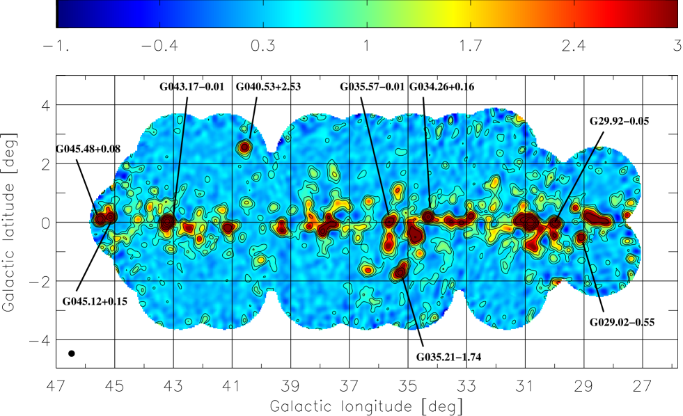
Figure 2: The 33 GHz map of the Galactic plane covering the region $\ell=27^{\circ}\!$ to $46^{\circ}\!$ and ${b}=-3^{\circ}.5$ to ${b}=+3^{\circ}.5$. Units are Jy beam^-1. Contour levels are at 0.5, 1, 2, 4, 8, 16, 32 and 64 per cent of the peak brightness (66.8 Jy beam^-1). The synthesized beam is shown in the lower left corner.

Frequency [GHz]	Telescope/Survey	Angular resolution [arcmin]	Reference
1.4	Effelsberg 100 m	9.4	Reich et al. (1990a)
2.7	Effelsberg 100 m	4.3	Reich et al. (1990b)
4.85	Green Bank 91 m	3.5	Condon et al. (1994)
8.35	Green Bank 13.7 m	9.4	Langston et al. (2000)
10.55	Nobeyama 45 m	3.0	Handa et al. (1987)
14.35	Green Bank 13.7 m	6.6	Langston et al. (2000)
94	WMAP	12.6	Hinshaw et al. (2009)
2997 (100 $\mu$m)	IRAS	4.3	Miville-Deschênes & Lagache (2005)
4995 (60 $\mu$m)	IRAS	4.0	Miville-Deschênes & Lagache (2005)
11990 (25 $\mu$m)	IRAS	3.8	Miville-Deschênes & Lagache (2005)
24980 (12 $\mu$m)	IRAS	3.8	Miville-Deschênes & Lagache (2005)

Table 3: The ancillary data used in this work.

Figure 3: Spectra of the 9 HII regions.The best-fit free-free spectrum through the 2.7 and 4.85 GHz data is shown (dotted line) for each region along with a 30 K thermal dust spectrum (dashed line) through the 100- $\mu$m and 60-$\mu$m data with $\beta=1.5$.

6 SPECTRA OF SELECTED HII REGIONS

We now consider the spectral characteristics of a selection of stronger objects in the 33 GHz survey. A wide selection of ancillary data ranging from 1.4 GHz to the FIR, is available for this purpose.

6.1 The ancillary data

For accurate spectral determination we require data from high signal-to-noise surveys covering the Galactic plane. Angular resolutions comparable to that of the VSA (13 arcmin) or better are required. The surveys satisfying these criteria are at 1.4, 2.7, 4.85, 8.35, 10.55, 14.35, 33, 94 GHz and the FIR bands at 100, 60, 25 and 12 $\mu$m and are listed in Table 3. It can be seen that high resolution data with resolutions $\sim 4-5$ arcmin are available at both radio and FIR wavelengths; these are particularly useful in the evaluation of the physical properties of the sources.

6.2 Modelling and mosaicing the ancillary data

In order to derive the spectrum of a source in the 33-GHz survey it is essential to compare the maps at different frequencies with the same resolution as the VSA observation. This is achieved by applying the same VSA $\it{u,v}$ coverage for each field, accounting for any flagged data. The procedure is undertaken in $\mathcal{AIPS}$ with the UVSUB task, followed by the imaging task IMAGR. When all the fields at each frequency have been modelled and imaged in this manner, they are mosaiced as for the 33-GHz data to provide a map at that frequency.

6.3 Selection of HII regions for detailed study

Some 60 sources can be identified in the 33-GHz map produced in the present investigation with peak flux densities $\geq 1.5$ Jy beam^-1. From this list we select the brightest objects in unconfused areas which are not contaminated by synchrotron sources, namely SNRs and extragalactic objects. The identification of the free-free and synchrotron sources is made on the evidence from the 2.7 GHz and 100 $\mu$m maps at the original resolution ($\sim 4^{\prime}$). The Green (2009) catalogue of SNRs was useful in this regard.

Several of the brightest features on the 33-GHz map such as G030.70-0.03 and G034.70-0.40 (the W44 region) had to be excluded because of their complexity and large extent; structures on scales $>40$ arcmin are affected by significant flux loss and are difficult to image due to limited u,v coverage. Furthermore, the differences between the diffuse synchrotron and free-free background distributions makes the determination of a spectral index difficult, even when the same (VSA) baselines are applied to the ancillary data.

Table 4 lists the 9 HII regions with flux densities that are determined with confidence. Integrated flux densities are given for the 8 radio frequencies used to derive the spectra of these HII regions, namely 1.4, 2.7, 4.85, 8.35, 10.55, 14.35, 33 and 94 GHz. The 33 GHz flux densities are all greater than 5 Jy. We note that the flux densities given for the HII component, A, of W49 could be derived accurately at the VSA resolution since it lies 12 arcmin from the SNR component, B.

6.4 Spectra of individual HII regions

The spectra of the 9 HII regions ranging from the radio to the FIR are plotted in Fig. 3. The sources of the radio and FIR data are given in Table 4. These data are convolved to the resolution of the VSA data as described in Section 6.2. The errors plotted for the individual observations are a conservative $\pm 20$ per cent of the flux density (Section 5.3). This value is appropriate given the observed scatter of data points, as described in Section 6.5.

These spectra will now be used to derive the free-free, thermal (large grains) dust and anomalous components of the emission in each HII region. The anomalous component will be assessed as an excess above the other two components plotted in Fig. 3.

6.5 Determining the free-free component

We use the lowest frequencies as reliable estimators of the free-free emission. Over the frequency range 1.4 to 33 GHz the flux density spectral index has a well-determined value of $\beta=-0.12$ (Dickinson et al., 2003). The data at 2.7 and 4.85 GHz are from well-calibrated surveys, with high ($\sim 4$ arcmin) resolution and hence provide the best estimators of the free-free emission. These frequencies are uncontaminated by dust (anomalous or thermal) emission.

A good test for the accuracy of the 2.7 and 4.85 GHz data, including any systematics in the analysis method, is to derive the average of the spectra normalized to the combined flux density at 2.7 and 4.85 GHz. The spectral index between 2.7 and 4.85 GHz is taken into account.

Fig. 4 shows this normalized spectrum for the 9 HII regions. The r.m.s. in the normalized flux density is shown as $\pm 1\sigma$. At 2.7 and 4.85 GHz the value of the $\sigma$ of the mean is less than 6 per cent while at the higher frequencies it is $7-11$ per cent, possibly representing the variation in the dust contribution between HII regions.

It can be seen that the mean 1.4 GHz flux density is slightly low ($\sim 0.90$) compared with the expected value of 1.00. This may represent a small degree of free-free self absorption. An HII region with a brightness temperature of $10^{3}$ K, and an electron temperature of 7000 K, would have a 1.4 GHz free-free optical depth of $\tau\simeq 0.15$ and a flux density of 0.85 of the optically thin value. The only HII region in this study exceeding this value is G045.12+0.14 which has $\tau=0.39$, consistent with dimensions of $1.5\times 0.5$ arcmin², found in the high resolution NVSS 1.4 GHz survey. At 2.7 and 4.85 GHz this source would have $\tau=0.08$ and $\tau=0.02$ respectively. On averaging with other HII regions the effect of self-absorption will be no more than $10$ per cent at 1.4 GHz and a few percent at 2.7 and 4.85 GHz. The agreement of the 1.4 GHz value with the normalized values confirms the accuracy of the calibration procedure adopted here.

Table 4: The predicted and observed integrated flux densities in Jy for the 9 sources. The letters O and P stand for “observed” and “predicted” integrated flux density, respectively. The predicted free-free flux density is estimated from the 2.7 and 4.85 GHz values. The excess, E, is the difference between the predicted and observed flux densities.

Source		1.4 GHz	2.7 GHz	4.85 GHz	8.35 GHz	10.55 GHz	14.35 GHz	33 GHz	94 GHz
G029.02$-0.55$	O	6.6	6.4	-	9.7	-	9.4	7.8	14.4
	P	6.9	6.4	-	5.6	-	5.2	4.7	4.2
	E	-0.3	0.0	-	+4.1	-	+4.2	+3.1	+10.2
G029.92$-0.05$	O	9.1	14.8	-	15.2	15.0	20.9	15.9	9.4
	P	15.4	14.8	-	12.4	12.1	11.7	10.5	9.3
	E	-6.3	0.0	-	+2.8	+2.9	+9.2	+5.4	+0.1
G034.26+0.16	O	8.9	15.1	15.8	22.1	27.7	29.5	18.3	20.9
	P	17.5	15.9	14.8	14.1	13.5	13.1	11.8	10.4
	E	-8.6	-0.8	+1.0	+8.0	+14.2	+16.4	+6.5	+10.5
G035.21$-1.74$	O	11.0	15.1	19.6	23.6	-	26.3	15. 6	22.1
	P	18.5	17.1	16.0	14.9	-	14.5	12.7	11.2
	E	-7.5	-2.0	+3.6	+8.7	-	+11.8	+2.9	+10.9
G035.57$-0.01$	O	30.8	25.6	14.1	14.6	25.1	24.6	15.0	22.4
	P	19.3	17.8	16.6	15.6	15.1	14.6	13.2	11.6
	E	+11.5	+7.8	-2.5	-1.0	+10.0	+10.0	+1.8	+10.7
G040.53+2.53	O	10.4	12.1	7.2	12.8	-	6.4	9.0	8.8
	P	9.8	9.0	8.4	7.9	-	7.4	6.7	5.9
	E	+0.7	+3.1	-1.2	+4.9	-	-1.0	+2.3	+2.9
G043.17$-0.01$	O	89.2	84.0	57.1	67.7	89.8	89.2	54.00	75.5
(W49)	P	74.8	69.2	64.5	59.5	57.8	55.7	51.2	45.2
	E	+14.4	+14.8	-7.4	+8.2	+32.0	+33.5	+2.8	+30.3
G045.12+0.15	O	4.5	6.8	5.3	11.2	11.0	11.0	9.4	9.8
	P	6.6	6.1	5.7	5.4	5.2	5.0	4.6	4.0
	E	-2.1	+0.7	-0.4	+5.8	+5.8	+6.0	+4.8	+5.8
G045.48+0.08	O	18.6	23.5	16.3	30.4	21.4	27.9	16.3	15.5
	P	21.2	19.6	18.3	17.1	16.7	16.1	14.5	12.8
	E	-2.6	+3.9	-2.0	+13.3	+4.7	+11.8	+1.8	+2.7
Mean of $\frac{\textbf{O}}{\textbf{P}}$		0.90$\pm$0.11	1.13$\pm$0.06	0.96$\pm$0.05	1.52$\pm$0.11	1.65$\pm$0.14	1.75$\pm$0.13	1.41$\pm$0.10	1.91$\pm$0.23
Mean of $\frac{\textbf{E}}{\textbf{P}}$		-0.10$\pm$0.11	0.09$\pm$0.06	-0.04$\pm$0.05	0.52$\pm$0.11	0.65$\pm$0.14	0.75$\pm$0.13	0.41$\pm$0.10	0.91$\pm$0.23

7 Anomalous emission in the selected HII regions

In this section we discuss the properties of the excess emission from the warm dust associated with 9 selected HII regions. These include some of the brightest HII regions in the Galaxy. We quantify the anomalous emission process as a function of radio frequency and of the FIR properties of the dust.

7.1 Excess emission at radio frequencies

The excess emission above the free-free emission for each HII region is defined and discussed in Sections  6.4 and  6.5. Basically the 2.7- and 4.85- GHz data define the HII spectrum, with confirmation by the 1.4 GHz data. Values of the predicted (P) free-free and the excess (E) flux densities are given in Table 4 for each of the 9 HII regions at each of the 8 spectral frequencies. The mean value of the ratio of the excess to the HII flux density (E/P) and its r.m.s. are given in Table 4 and plotted for the 8 frequencies in Fig. 5.

Figure 4: The ratio of observed integrated flux density, $S_{O}$, to that of the predicted free-free, $S_{P}$, for the 8 frequencies. Unity is the value for the free-free alone, based on 2.7 and 4.85 GHz mean flux densities. $1\sigma$ errors are shown.

Figure 5: The average ratios of the excess emission, $S_{E}$, to the predicted free-free flux density, $S_{P}$, as a function of frequency. $1\sigma$ errors are shown.

The excess emission at frequencies in the range 8.35 to 94 GHz is clearly seen. At individual frequencies there is a scatter between the HII regions of $\sim 25$ per cent about the mean; this will include a measurement error and will have a component due to differences in the emission process in HII regions. The 33 GHz excess relative to the HII emission has the smallest scatter. At this frequency the excess is $41\pm 10$ per cent of the free-free emission. It is interesting to note that the bright diffuse emission on the Galactic plane has a similar ratio of anomalous to free-free emission (Kogut et al. 2009; Alves et al. 2010).

The 94 GHz excess relative to the free-free has the highest value. As we shall demonstrate below, this excess is due to thermal (vibrational) emission from the larger dust grains. The spinning dust spectrum is not expected to extend up to such high frequencies or at least will be small at 94 GHz (Ali–Haïmoud et al. 2009).

7.2 33 GHz excess compared with FIR bands

We now compare the 33-GHz data with the IRAS FIR bands since there is a substantial body of data (ground-based and WMAP), which should provide a comprehensive picture of anomalous emission properties at a frequency near the centre of the emission spectrum of spinning dust.

As we shall see below (Section 8.3), there is a strong correlation between the 4 IRAS bands. However, they represent different types of dust; the 60- and 100-$\mu$m bands are from larger grains, while the 25- and 12-$\mu$m bands are from very small grains (VSGs) and polycyclic aromatic hydrocarbons (PAHs). The spinning dust emission is from the latter grains.

Table 5 lists the flux densities for the 9 HII regions in the 33 GHz and the four IRAS bands. The 33 GHz excess is also given as a ratio to the IRAS flux densities. The mean values and the errors of these ratios for the 4 IRAS bands are listed. It can be seen that there is a marginally smaller scatter of the 33 GHz excess with the 25- and 12-$\mu$m bands ($6.0\sigma$ and $5.8\sigma$) than with the 100- and 60-$\mu$m bands ($5.4\sigma$ and $5.0\sigma$). Such a difference would be expected in a spinning dust scenario.

Fig. 6 shows this scatter in the distribution of 33 GHz excess relative to the FIR emission in the 4 IRAS bands. It is likely that the bulk of the scatter is due to the 33-GHz data; the radio and FIR emission is co-located as indicated in the positions of the individual HII regions (Section 8.1). For example G045.12+0.15 is high relative to the rest of the sample. This could be due to systematics in the 33 GHz data or differences in intrinsic spinning dust emission at 60 and 100 $\mu$m.

Figure 6: Histograms (a), (b), (c) and (d) showing the spread in the ratio of the excess 33 GHz integrated flux density to those of the IRAS bands at 100, 60, 25 and 12 $\mu$m, respectively. The vertical solid and the dotted lines show the mean and the 1 $\sigma$ values respectively.

7.3 The anomalous radio spectrum relative to the 100 micron dust emission

The ratio of the radio emission relative to FIR dust emission expressed as a flux density or surface brightness is commonly used as an indicator of the strength of the anomalous emission. We now use our radio data covering 8 frequencies in the range 1.4 to 94 GHz to derive a spectrum for the dust-correlated radio emission relative to the 100 $\mu$m emission. The ratio of excess radio to total 100 $\mu$m flux density in each of the 8 frequency bands is given for the 9 HII regions in Table 6.

Table 6 also lists the radio emissivity relative to 100 $\mu$m at each frequency, averaged across the 9 HII regions. Fig. 7 shows the resulting spectrum of excess emissivity in the frequency range 1.4 to 94 GHz. We will argue below that the 94 GHz is mostly thermal (vibrational) emission from large grains rather than spinning dust emission.

Fig. 7 illustrates the central result of this investigation. It defines the spectrum of warm dust in HII regions which can be compared with that of cool dust clouds (Watson et al., 2005; Casassus et al., 2006). The figure also shows the Draine & Lazarian (1998) model for the warm ionized medium (WIM). Our data would give a better fit if the WIM spectrum were moved to frequencies lower by a factor of $0.68$. A wide range of spectral shapes are predicted by Ali-Haïmoud et al. (2009), some of which give a better fit to the data. A shift in the position of the peak could also indicate different chemical compositions (Iglesias-Groth, 2005). We note that the lowest peak frequencies observed theoretically, are $\sim 15$ GHz (Ali-Haïmoud et al. 2009), similar to what is observed in Fig. 7. Also, the WIM model of Ysard & Verstraete (2010) had the lowest peak frequency ($\sim 20$ GHz) of the models representing typical ISM environments.

7.4 Comparison of the present VSA results with other 30-GHz measurements

We first consider the anomalous emission from HII regions. A summary of the published data is given in Table 7. These include the CBI results (Dickinson et al., 2006, 2007, 2009) at 31 GHz. These have been converted to emissivities in $\mu$K (MJy/sr)^-1 at 33 GHz for comparison with the present data. In the case of RCW175 the results for its two components are given separately. We note that the VSA flux density (7.8 Jy) is somewhat greater than that given by the CBI (5.97 Jy). This probably results from the fact that the CBI has resolved out some of the extended emission.

There is clearly good consistency between the results for the warm dust clouds associated with HII regions in the various investigations. The weighted average emissivity is $4.65\pm 0.40$ (11.6 $\sigma$) $\mu$K (MJy/sr)^-1 at 33 GHz.

It is of particular interest to compare the radio emissivity of the warm ($\sim 40$ K) dust in HII regions with that in the general field where dust temperatures are typically $\sim 20$ K. The data, corrected to 33 GHz where necessary, are given in Table 8.

Table 5: The comparison of the 33 GHz excess for the 9 HII regions relative to the integrated flux densities in the four IRAS bands. Column 1 lists the sources, columns 2 and 3 list the observed ($S_{33}$) and the excess ($\Delta S_{33}$) flux densities at 33 GHz. The observed flux densities in the IRAS bands are shown in columns 4-7. Columns 8-12 list the ratios of the excess flux densities at 33 GHz to the flux densities at 100, 60, 25 and 12$\mu$m. The mean ratios of 33 GHz excess relative to the IRAS flux densities is given in heavy type.

	$S_{33}$	$\Delta S_{33}$	$S_{100}$	$S_{60}$	$S_{25}$	$S_{12}$	$\frac{\Delta S_{33}}{S_{100}}$	$\frac{\Delta S_{33}}{S_{60}}$	$\frac{\Delta S_{33}}{S_{25}}$	$\frac{\Delta S_{33}}{S_{12}}$
Source	[Jy]	[Jy]	$\times 10^{4}$ [Jy]	$\times 10^{4}$ [Jy]	$\times 10^{2}$ [Jy]	$\times 10^{2}$ [Jy]	$\times 10^{-4}$	$\times 10^{-4}$	$\times 10^{-4}$	$\times 10^{-4}$
1	2	3	4	5	6	7	8	9	10	11
G029.02$-$0.55	7.8 $\pm$1.6	+3.1$\pm$1.7	1.8$\pm$0.4	1.1$\pm$0.2	9.1$\pm$2.0	7.0$\pm$1.4	1.72	2.82	20.2	44.3
G029.92$-$0.05	15.9$\pm$3.2	+5.4$\pm$3.5	3.8$\pm$0.8	2.9$\pm$0.6	49.1$\pm$9.8	7.4$\pm$1.5	1.42	1.86	11.0	73.3
G034.26+0.16	18.3$\pm$3.7	+6.5$\pm$4.0	5.5$\pm$1.1	3.5$\pm$0.7	39.4$\pm$7.9	5.5$\pm$1.1	1.18	1.86	16.5	118.4
G035.21$-$1.74	15.6$\pm$3.1	+2.9$\pm$3.6	3.7$\pm$0.7	3.0$\pm$0.6	46.3$\pm$9.3	9.8$\pm$2.0	0.78	0.97	6.3	29.6
G035.57$-$0.01	15.0$\pm$3.0	+1.8$\pm$3.6	2.7$\pm$0.5	1.7$\pm$0.3	15.8$\pm$3.2	3.3$\pm$0.7	0.67	1.06	11.4	54.9
G040.53+2.53	9.0$\pm$1.8	+2.3$\pm$3.0	2.6$\pm$0.5	1.8$\pm$0.4	25.2$\pm$5.0	4.8$\pm$1.0	0.88	1.28	9.1	47.6
G043.17$-$0.01	54.0$\pm$10.8	+2.8$\pm$1.2	6.8$\pm$1.4	4.5$\pm$0.9	75.0$\pm$15.0	8.2$\pm$1.6	0.41	0.62	3.7	34.2
G045.12+0.15	9.4$\pm$2.0	+4.8$\pm$2.0	2.1$\pm$0.4	1.3$\pm$0.3	38.9$\pm$7.8	5.9$\pm$1.2	2.29	3.63	12.3	81.6
G045.48+0.08	16.3$\pm$3.3	+1.8$\pm$3.9	4.8$\pm$1.0	3.1$\pm$0.6	45.6$\pm$9.1	8.8$\pm$1.8	0.38	0.58	3.9	20.6
Mean							1.08$\pm$0.20	1.63$\pm$0.32	10.5$\pm$1.7	56.1$\pm$ 9.6
$\sigma$							5.4$\sigma$	5.0$\sigma$	6.0$\sigma$	5.8$\sigma$

The all-sky WMAP analysis with the Kp2 mask refers to dust at intermediate and high Galactic latitudes (Davies et al., 2006) where the 15 regions included the brighter FIR dust clouds at intermediate latitudes on scales of $1^{\circ}-5^{\circ}$. The more compact regions G159.6$-$18.5 and LDN 1622 each contain fine structure and relatively weak associated HII regions; they have the highest emissivity.

In summary, the 33 GHz emissivity of HII region dust clouds is $\sim 40$ per cent of that of dust in the diffuse and extended ISM and is $\sim 20$ per cent of that in more compact dust clouds. We will discuss possible reasons for these different emissivities in Section 9.

8 Other physical properties of the 9 HII regions

We have further data at the 8 radio frequencies and 4 FIR frequencies which can be used to derive additional physical properties of the 9 HII regions - positions, diameters, SEDs and dust temperatures.

8.1 Radio positions relative to the dust

We use the 2.7 GHz data to define the position of the free-free emission and the 100 $\mu$m IRAS data for the dust. In order to directly intercompare the 33 GHz data, the 13 arcmin smoothed positions at 2.7 GHz and 100  $\mu$m are used since a number of HII regions have complex structures. Fig. 8 shows the relative positions at 2.7 GHz, 33 GHz and 100 $\mu$m for the 9 HII regions.

The mean of the offsets, excluding RCW175, are shown in Fig. 8 as dashed lines. The offset between 33 GHz and 100 $\mu$m positions is $(\Delta\ell,\Delta\emph{b})=(-0.13,-0.33)$ arcmin. The offsets from 2.7 GHz are larger; the offset from 33 GHz is $(\Delta\ell,\Delta\emph{b})=(1.18,-0.34)$ arcmin and from 100 $\mu$m is $(\Delta\ell,\Delta\emph{b})=(-1.44,-0.05)$ arcmin. The 2.7 GHz positions appear to be displaced by $\sim 1.2$ arcmin from those at 33 GHz and 100 $\mu$m. There is no obvious reason for this displacement; the 2.7 GHz positions are accurate to $20$ arcsec in $\ell$ and $33$ arcsec in $\it{b}$ (Reich et al., 1990b).

The scatter about the mean offset is similar for each of the 3 comparisons with an r.m.s. of $1.5$ arcmin, excluding RCW175 (triangle). This scatter results from the noise on the 3 maps.

These results indicate that the free-free and the dust components agree in position to $\pm 1$ arcmin when the 2.7 GHz offset is allowed for. The tight correlation between the 33 GHz and 100 $\mu$m confirms this result since $\sim 70$ per cent of the 33 GHz emission is due to free-free and $\sim 30$ per cent is from anomalous emission (see Table 4).

8.2 Radio diameters relative to the dust

The 2.7 GHz, 33 GHz and 100 $\mu$m data, at the $13$ arcmin resolution of the VSA beam, can be used to intercompare the diameters of the free-free and dust emission in the 9 HII regions. Fig. 9 shows this intercomparison. The diameters are determined for Gaussian fits to the emission. They are the intrinsic diameters derived from the beam broadening observed. Diameters less than $3$ arcmin will be uncertain; they broaden the beam by $\leq 0.4$ arcmin.

Figure 7: The spectrum of the averaged radio emission relative to 100 $\mu$m emission for the 9 HII regions. The values are in units of $10^{-4}$ and the plotted errors are $1\sigma$. The dotted curve is the DL98 model for rotational emission from a spinning dust grains in warm ionized medium (WIM). The solid line is the same model shifted by a factor of $0.68$ to lower frequencies.

Table 6: The comparison of the excess radio flux density relative to 100 $\mu$m from 1.4 to 94 GHz for the 9 HII regions. All ratios are given in units of $\times 10^{-4}$.

Source	$\frac{\Delta S_{1.4}}{S_{100\mu}}$	$\frac{\Delta S_{2.7}}{S_{100\mu}}$	$\frac{\Delta S_{4.85}}{S_{100\mu}}$	$\frac{\Delta S_{8.35}}{S_{100\mu}}$	$\frac{\Delta S_{10.55}}{S_{100\mu}}$	$\frac{\Delta S_{14.35}}{S_{100\mu}}$	$\frac{\Delta S_{33}}{S_{100\mu}}$	$\frac{\Delta S_{94}}{S_{100\mu}}$
G029.02$-$0.55	$-0.17$	0.00	-	2.28	-	2.33	1.72	5.67
G029.92$-$0.05	$-1.66$	0.00	-	0.74	0.76	2.42	1.42	0.03
G034.26$+$0.16	$-1.56$	$-0.15$	0.18	1.45	2.58	2.98	1.18	1.91
G035.21$-$1.74	$-2.03$	$-0.54$	0.97	2.35	-	3.19	0.78	2.95
G035.57$-$0.01	4.26	2.89	$-0.93$	$-0.37$	3.70	3.70	0.67	3.96
G040.53$+$2.53	0.27	1.19	$-0.46$	1.88	-	$-0.38$	0.88	1.12
G043.17$-$0.01	2.12	2.18	$-1.09$	1.21	4.71	4.93	0.41	4.46
G045.12$+$0.15	$-1.00$	0.33	$-0.19$	2.76	2.76	2.86	2.29	2.76
G045.48$+$0.08	$-0.54$	0.81	$-0.42$	2.77	0.98	2.46	0.38	0.56
Mean	0.31$\pm$0.63	0.75$\pm$0.36	-0.28$\pm$0.24	1.67$\pm$0.33	2.58$\pm$0.57	2.72$\pm$0.45	1.08$\pm$0.20	2.60$\pm$0.59
$\sigma$	0.5$\sigma$	2.1$\sigma$	1.1$\sigma$	5.1$\sigma$	4.2$\sigma$	6.1$\sigma$	5.4$\sigma$	4.3$\sigma$

Table 7: Comparison of 33 GHz radio emissivities, relative to $100~{}\mu$m, of dust in HII regions.

HII regions	Instrument	Dust emissivity (33 GHz)	Reference
		$\mu$K (MJy/sr)-1
6 Southern HII regions	CBI	$2.9\pm 1.5$	Dickinson et al.(2007)
LPH96	CBI	$5.2\pm 2.1$	Dickinson et al.(2006)
G029.01$-$0.6	CBI	$4.7\pm 0.9$	Dickinson et al.(2009)
G029.01$-$0.7	CBI	$6.8\pm 1.1$	Dickinson et al.(2009)
9 Northern HII regions	VSA	$3.9\pm 0.8$	This work
Weighted average		$4.65\pm 0.40$ (11.5$\sigma$)

Table 8: Comparison of 33 GHz emissivities relative to 100 $\mu$m in cool (field) and warm (HII region) dust clouds.

Region	Instrument	Dust emissivity (33 GHz)	Morphology	Reference
		$\mu$K (MJy/sr)-1	Size
G159.6-18.5	COSMOSOMAS	$17.8\pm 0.3$	$1^{\circ}.6\times 1^{\circ}.0$	Watson et al. (2005)
LDN1622	CBI	$21.3\pm 0.6$	$<10$ arcmin	Casassus et al. (2006)
15 WMAP regions	WMAP	$11.2\pm 1.5$	$1^{\circ}-5^{\circ}$	Davies et al. (2006)
All-sky WMAP (Kp2)	WMAP	$10.9\pm 1.1$	Diffuse	Davies et al. (2006)
HII regions (mean)		$4.65\pm 0.40$ (11.5$\sigma$)		This work

Figure 8: Relative position offsets of the 9 HII regions at 2.7 GHz, 33 GHz and 100 $\mu$m dust. (a) the 100 $\mu$m relative to 33 GHz. (b) 2.7 GHz relative to 33 GHz (c) 2.7 GHz relative to 100 $\mu$m. The the dashed lines show the mean offset in each plot, excluding RCW175.

Figure 9: Comparison of the deconvolved 33 GHz dimensions of HII regions to those at (a) 100 $\mu$m, (b) 25 $\mu$m and (c) 2.7 GHz . The 2.7 GHz (free-free) dimensions are compared to those of dust (100 $\mu$m) in (d). Major and minor axes diameters are given in each plot.

The intercomparison of the 2.7 GHz, 33 GHz and the 100 $\mu$m data shows close similarity of diameters at these 3 wavelengths. The tight correlation between the 2.7 GHz (free-free) and the 100 $\mu$m (dust) diameters emphasizes the close agreement in the spatial distribution of these 2 ISM components.

The agreement between the free-free and dust positions along with the similarity of the diameters shows that ionized gas and warm dust are well mixed in HII regions. This is not the situation in the general ISM as was found in the 15-region investigation (Davies et al., 2006).

8.3 The radio - FIR spectrum of warm thermal dust in HII regions

We now determine the SED of thermal dust in HII regions extending from 94 GHz, where the excess due to dust is unambiguously detected at radio frequencies, to the IRAS FIR frequencies. Table 9 shows the mean flux density ratio of the 4 bands relative to the 100 $\mu$m values for the 9 HII regions.

Table 9: The summary table of the mean emissivities in the IRAS bands and the 94 GHz excess emission with respect to 100 $\mu$m thermal dust. Note that the 94 GHz value should be multiplied by $10^{-4}$.

	$\frac{\Delta S_{94GHz}}{S_{100\mu\rm{m}}}$	$\frac{S_{60\mu\rm{m}}}{S_{100\mu\rm{m}}}$	$\frac{S_{25\mu\rm{m}}}{S_{100\mu\rm{m}}}$	$\frac{S_{12\mu\rm{m}}}{S_{100\mu\rm{m}}}$
Mean	$2.60$	$0.67$	$0.103$	$0.0203$
$\sigma$	$4.4\sigma$	$30.2\sigma$	$7.9\sigma$	$7.1\sigma$

It is clear that the 60 $\mu$m and 100 $\mu$m values are tightly correlated (at $30\sigma$) while the 25 $\mu$m and 12 $\mu$m are less correlated with 100 $\mu$m (at $7.9\sigma$ and $7.1\sigma$, respectively). The 94 GHz dust emission shows a significant ($4.4\sigma$) detection of the long wavelength dust emission. The scatter may be due to variation in the emissivity index $\beta$ between the 9 dust clouds.

Figure 10: The mean emissivities of the 9 HII regions in the IRAS bands and the 94 GHz excess emission with respect to 100 $\mu$m thermal dust. The $\beta=$1.5, 1.7 and 2.0 spectra for thermal dust are shown separately. The best fit is for a dust temperature of 39 K and $\beta=1.5$.

Fig. 10 is the plot of the SED relative to 100 $\mu$m of the warm dust in the 9 HII regions of the present study. Also plotted are spectra through the 60 and 100 $\mu$m points for assumed dust emissivity indices of $\beta=$1.5, 1.7 and 2.0. The best fitting dust temperature, which includes the 94 GHz value, is 39 K for $\beta=+1.5$. The very small grain dust emission represented by the 12 $\mu$m and 25 $\mu$m points shows as an excess above the extrapolated large grain dust emission.

8.4 Temperature dependence of relevant parameters

The IRAS data can also be used to derive the dust temperature of each HII region. Kuiper et al. (1987) give recipes for deriving the temperature of the large grain component in the normal ISM environment, using the 60 and 100 $\mu$m data. This treatment assumes a value of $\beta$ and does not take account of the 94 GHz in determining $\beta$. It is a complex process to determine an accurate dust temperature (e.g. Dupac et al. 2003), so accordingly we will adopt the ratio, R, of 60 $\mu$m to 100 $\mu$m flux density as a temperature indicator in our investigation of dust properties. A higher value of R represents a higher temperature. The parameters considered are the anomalous emission ($\Delta S_{33\textrm{GHz}}/S_{100\mu\textrm{m}}$), the thermal dust ($\Delta S_{94\rm{GHz}}/S_{100\mu\rm{m}}$) and the free-free emission ($S^{ff}_{33\rm{GHz}}/S_{100\mu\rm{m}}$). The values of each parameter are listed in Table 10.

Table 10: The parameters used for investigating temperature dependences in the 9 HII regions. R, the ratio between the 60 $\mu$m and the 100 $\mu$m flux densities, is the temperature indicator.

	R	$\frac{\Delta S_{33\rm{GHz}}}{S_{100\mu\rm{m}}}$	$\frac{S^{ff}_{33\rm{GHz}}}{S_{100\mu\rm{m}}}$	$\frac{\Delta S_{94\rm{GHz}}}{S_{100\mu\rm{m}}}$	$\frac{S_{25\mu\rm{m}}}{S_{100\mu\rm{m}}}$
Source		$\times 10^{-4}$	$\times 10^{-4}$	$\times 10^{-4}$	$\times 10^{-4}$
G029.02$-$0.55	0.60	1.72	2.61	5.67	0.051
G029.92$-$0.05	0.76	1.42	2.76	0.03	0.129
G034.26+0.16	0.64	1.18	2.14	1.91	0.072
G035.21$-$1.74	0.81	0.78	3.43	2.95	0.125
G035.57$-$0.01	0.63	0.67	4.89	3.96	0.059
G040.53+2.53	0.69	0.88	2.58	1.12	0.097
G043.17$-$0.01	0.66	0.41	7.53	4.46	0.110
G045.12+0.15	0.62	2.29	2.19	2.76	0.185
G045.48+0.08	0.65	0.38	3.02	0.56	0.095
Mean		$1.08\pm 0.20$	$3.46\pm 0.55$	$2.60\pm 0.59$	$0.103\pm 0.0131$
$\sigma$		$5.4\sigma$	$6.3\sigma$	$4.4\sigma$	$7.9\sigma$

Fig. 11 (a) shows the anomalous emission for each of the 9 HII regions as a function of R, the ratio between the 60 and 100 $\mu$m flux densities. This plot shows a weak correlation ($2.6\sigma$) with a decrease in $\Delta S_{33\textrm{GHz}}/S_{100\mu\textrm{m}}$ as a function of temperature. Such a decrease would be caused by a greater 100 $\mu$m emission per unit dust density at higher temperatures - as expected.

Figure 11: The temperature dependence of (a) anomalous emission, (b) free-free emission and (c) 94 GHz. The temperature indicator, R, is the ratio of 60 $\mu$m to 100 $\mu$m flux density.

Fig. 11 (b) shows the free-free emission at 33 GHz relative to 100 $\mu$m as a function of temperature. A modest positive correlation is found suggesting the level of free-free increases more rapidly with temperature than the dust at 100 $\mu$m. There is no obvious physical reason for this.

Fig. 11 (c) shows the 94 GHz thermal dust emission relative to 100 $\mu$m as a function of temperature. This shows the strongest correlation of the study. Such a negative correlation could be due to a $\beta$ variation with temperature in the thermal emission spectrum and/or the increase in 100 $\mu$m emission with temperature, as expected for thermal dust emission.

9 Conclusions

We have presented here a high sensitivity 33 GHz map made with the VSA of a $19^{\circ}$ section of the northern Galactic plane covering $\ell=27^{\circ}$ to $46^{\circ}$. The VSA detects structure up to a scale of $\sim 50$ arcmin with a resolution of $13$ arcmin; scales $>50$ arcmin are resolved out. The major part of this structure detected at 33 GHz is free-free emission from HII regions. This data set is combined with 7 other surveys in the frequency range 1.4 to 94 GHz and IRAS data at 100, 60, 25 and 12 $\mu$m to investigate the physical properties of the warm dust and ionized gas in 9 well-defined HII regions detected in the survey.

A significant outcome of this investigation is the clear detection of anomalous dust-correlated emission in HII regions. When combined with published data on individual HII regions the 33 GHz relative to the 100 $\mu$m brightness is $4.65\pm 0.40$ $\mu$K (MJy/sr)^-1 ($11.5\sigma$). This value is 3-5 times less than that of cool (20 K) dust in the field. This lower radio/FIR emissivity in the warm clouds most likely arises from the fact that the 100 $\mu$m brightness increases as $T^{4}$ while the 33 GHz emission depends on the surface density of dust grains only. Further investigation is required.

The combined radio data set has been used to determine the spectrum of the excess emission in the warm HII region dust clouds. The mean spectrum of this excess emission relative to the 100 $\mu$m emission is found to peak in the region of 20 GHz. Although the spectrum is offset in frequency relative to the Draine & Lazarian prediction for the warm interstellar medium, other predictions are available (Ali-Haïmoud et al. 2009) which may throw light on the physical conditions necessary for the anomalous emission.

The 33 GHz survey of HII regions on the Galactic plane has shown the close association between warm dust and free-free emission; the dust and ionized gas appear well-mixed on arcmin scales. Our survey has also permitted the identification of the thermal (vibrational) component of emission at 94 GHz which provides a measure of the dust emission at short radio wavelengths. This is an area where Planck (Tauber et al., 2010) measurements will provide a definitive spectrum of the radio SED of dust, both in the Galactic plane and at intermediate latitude. Finally, we have found only weak correlations between the dust temperature and such parameters as anomalous radio emissivity, free-free emission and 94 GHz emission; these correlations, although weak, probably result from the expected higher FIR emission per unit dust density at higher temperatures.

10 Acknowledgments

We thank the anonymous referee for useful comments on the paper. We thank the staff of Jodrell Bank Observatory, Mullard Radio Astronomy Observatory and the Teide Observatory for assistance in the day-to-day operation of the VSA. We are very grateful to PPARC (now STFC) for the funding and support for the VSA project and the Instituto de Astrofísica de Canarias (IAC) for supporting and maintaining the VSA in Tenerife. Partial financial support was provided by the Spanish Ministry of Science and Technology project AYA2001-1657. CD acknowledges an STFC Advanced Fellowship and ERC grant under the FP7. YAH thanks the King Abdulaziz City for Science and Technology for support. YAH also thanks His Highness Prince Dr Turki Bin Saud Bin Mohammad Al Saud for his personal support. JAR-M is a Ramón y Cajal fellow of the Spanish Ministry of Science and Innovation (MICINN).

References

- (1) Ali-Haïmoud Y., Hirata C.M., Dickinson C., 2009, MNRAS, 395, 1055
- (2) Alves M. I. R., Davies R. D., Dickinson C., Davis R.J., Auld R. R., Calabretta M., Staveley-Smith L., 2010, MNRAS, submitted (arXiv:0912.2290)
- (3) Banday A.J., Dickinson C., Davies R.D., Davis R.J., Górski K.M., 2003, MNRAS, 345, 897
- Casassus et al. (2006) Casassus, S., Cabrera, G. F., Förster, F., Pearson, T. J., Readhead, A. C. S., & Dickinson, C. 2006, ApJ, 639, 951
- (5) Condon J.J., Broderick J.J., Seielstad G.A., Douglas K., Gregory P.C., 1994, AJ, 107, 1829
- de Oliveira-Costa et al. (1999) de Oliveira-Costa, A., Tegmark, M., Gutierrez, C. M., Jones, A. W., Davies, R. D., Lasenby, A. N., Rebolo, R., & Watson, R. A. 1999, ApJ, 527, L9
- de Oliveira-Costa et al. (2002) de Oliveira-Costa, A., et al. 2002, ApJ, 567, 363
- (8) de Oliveira-Costa A., Tegmark M., Davies R.D., Gutiérrez C.M., Lasenby A.N., Rebolo R., Watson R.A., 2004, ApJ, 606, L89
- (9) Davies R.D., Dickinson C., Banday A.J., Jaffe T.R., Górski K.M., Davis R.J., 2006, MNRAS, 370, 1125
- (10) Dickinson C., Davies R.D., Davis R.J., 2003, MNRAS, 341, 369
- (11) Dickinson, C. et al. 2004, MNRAS, 353, 732
- (12) Dickinson C., Casassus S., Pineda J.L., Pearson T.J., Readhead A.C.S., Davies R.D., 2006, ApJL, 643, L111
- (13) Dickinson C., Davies R.D., Bronfman L., Casassus S., Davis R.J., Pearson T.J., Readhead A.C.S., Wilkinson P.N., 2007, MNRAS, 379, 297
- (14) Dickinson C. et al. 2009, ApJ, 690, 1585
- (15) Draine B.T., Lazarian A., 1998, ApJ, 494, L19
- Dupac et al. (2003) Dupac, X., et al. 2003, A&A, 404, L11
- (17) Finkbeiner D.P., Schlegel D.J., Curtis F., Heiles C., 2002, ApJ, 566, 898
- Finkbeiner (2004) Finkbeiner, D. P. 2004, ApJ, 614, 186
- (19) Green D.A., BASI, 2009, 37, 45
- (20) Hafez Y.A. et al. 2008, MNRAS, 388, 1775
- (21) Handa T., Sofue Y., Nakai N., Hirabayashi H., Inoue M., 1987, PASJ, 39, 709
- (22) Hill R.S. et al. 2009, ApJS, 180, 246
- (23) Hinshaw, G. et al. 2009, ApJS, 180, 225
- (24) Högbom J.A., 1974, A&AS, 15, 417
- Iglesias-Groth (2005) Iglesias-Groth, S. 2005, ApJ, 632, L25
- (26) Kogut A., Banday A.J., Bennett C.L., Gorski K.M., Hinshaw G., Smooth G.F., Wright E.I., 1996, ApJ, 464, L5
- (27) Kogut A. et al. 2009, ApJ, submitted (arXiv:0901.0562)
- (28) Kuiper T.B.H., Whiteoak J.B., Fowler J.W., Rice W., 1987, MNRAS, 227, 1013
- (29) Lagache G., 2003, A&A, 405, 813
- (30) Langston G., Minter A., D’Addario L., Eberhardt K., Koski K., Zuber J., 2000, AJ, 119, 2801
- (31) Leitch E.M., Readhead A.C.S., Pearson T.J., Myers S.T., 1997, ApJ, 486, L23
- (32) Maisinger K., Hobson M.P., Saunders R.D.E., Grainge K.J.B., 2003, MNRAS, 345, 800
- (33) Miville-Deschênes M.-A., Lagache G., 2005, ApJS, 157, 302
- (34) Reich W., Reich P., Fürst E., 1990a, A&AS, 83, 539
- (35) Reich, W., Fürst, E., Reich, P., Reif, K., 1990b, A&AS, 85, 633
- Scaife et al. (2008) Scaife, A. M. M., et al. 2008, MNRAS, 385, 809
- Scaife et al. (2009) Scaife, A. M. M., et al. 2009, MNRAS, 400, 1394
- (38) Scott P.F. et al. 2003, MNRAS, 341, 1076
- Shepherd (1997) Shepherd, M. C. 1997, Astronomical Data Analysis Software and Systems VI, Astron. Soc. Pac., San Francisco, Hunt G. and Payne H.E. eds., 125, 77
- Tauber (2010) Tauber, J. A., et al., 2010, A&A, submitted
- Tibbs et al. (2010) Tibbs, C. T., et al. 2010, MNRAS, 402, 1969
- (42) Watson R.A. et al. 2003, MNRAS, 341, 1057
- (43) Watson R.A., Rebolo R., Rubiño-Martín J.A., Hildebrandt S., Gutiérrez C.M., Fernández-Cerezo S., Hoyland R.J, Battistelli E.S., 2005, ApJ, 624, L89
- (44) Ysard, N., & Verstraete, L. 2010, A&A, 509, A12
- (45)