Experimental Examination of the Effect of Short Ray Trajectories in Two-port Wave-Chaotic Scattering Systems

Abstract

Abstract

Predicting the statistics of realistic wave-chaotic scattering systems requires, in addition to random matrix theory, introduction of system-specific information. This paper investigates experimentally one aspect of system-specific behavior, namely the effects of short ray trajectories in wave-chaotic systems open to outside scattering channels. In particular, we consider ray trajectories of limited length that enter a scattering region through a channel (port) and subsequently exit through a channel (port). We show that a suitably averaged value of the impedance can be computed from these trajectories and that this can improve the ability to describe the statistical properties of the scattering systems. We illustrate and test these points through experiments on a realistic two-port microwave scattering billiard.

PACS Numbers

05.45.Mt Quantum chaos; semiclassical methods

03.65.Nk Scattering theory

03.65.Sq Semiclassical theories and applications

05.60.Gg Quantum transport

I Introduction

Random matrix theory (RMT) has achieved substantial success at predicting short wavelength statistical properties of spectra, eigenfunctions, scattering matrices, impedance matrices, and conductance of wave-chaotic systems Verb ; Mehta ; Beenakker_review_RMT ; Stock ; Fyodorov . By wave-chaotic systems, we mean that the behavior of the wave system in the small wavelength limit is described by ray orbit trajectories that are chaotic S1 . In practice, the experimental applicability of RMT requires consideration of nonuniversal effects. For example, in the particular case of scattering, the scattering properties of an open system depend on the coupling between the field within the scattering region and the asymptotic incoming and outgoing waves connecting the exterior to the scatterer. For this problem, researchers have developed methods to incorporate nonuniversal coupling and port-specific effects into the analysis of short wavelength scattering data for systems whose closed classical counterparts are ray-chaotic Poisson_Kernel_Original ; Brouwer_Lorentzian ; Poisson_including_internal ; Kuhl ; S1 ; Henry_paper_one_port ; Henry_paper_many_port ; Richter ; Haake .

Previous comparisons of experimental data to RMT have often employed ensembles of realizations of the system to compile statistics. To create such ensembles, researchers have typically varied the geometrical configuration of the scattering region and/or taken measurements at several different wavelengths Henry_paper_one_port ; Henry_paper_many_port ; S1 ; Schafer . These variations aim to create a set of systems in which none of the nonuniversal system details are reproduced from one realization to another, except for the effects of the port details. Thus, by suitably accounting for the port details, it was hoped that only universal RMT properties remained in the ensemble data. However, there can be problems in practice. For example, in the case of geometrical configuration variation, researchers typically move perturbing objects inside a ray-chaotic enclosure with fixed shape and size S1 ; Henry_paper_one_port ; Henry_paper_many_port , or move one wall of that enclosure Schafer , to create an ensemble of systems with varying details. The problem is that certain walls or other scattering objects of the enclosure remain fixed throughout the ensemble. Therefore, there may exist relevant ray trajectories that remain unchanged in many or all realizations of the ensemble. We term such ray trajectories that leave a port and soon return to it (or another port) before ergodically sampling the enclosure “short ray trajectories”.

A similar problem arises for wavelength variation in which a band of wavelengths is used. Within a wavelength range, if a ray trajectory length is too short, then the variation of the phase accumulated by a wave following that trajectory may not be large enough to be considered random. In such a case the effects of specific (hence, nonuniversal) short ray trajectories will survive the ensemble averaging processes described above. These problems will make systematic, nonuniversal contributions to the ensemble data, and thus consideration of short ray trajectories arises naturally in the semiclassical approach to quantum scattering theory wirtz ; Richter ; Haake ; Nazmitdinov ; Stampfer ; ishio_and_burgdoerfer ; Stein ; ishio_and_keating ; prange_alone ; gutzwiller_book ; Stock . Such short-ray-trajectory contributions have been noted before in microwave billiards Henry_paper_one_port ; Henry_paper_many_port ; ZSO or for quantum transport in chaotic cavities Richter ; Haake and have either constrained or frustrated previous tests of RMT predictions.

By a “short ray trajectory” we mean one whose length is not much longer than several times the characteristic size of the scattering region, and which enters the scattering region from a port, bounces (perhaps several times) within the scattering region, and then returns to a port. A “port” is the region in which there is a connection from the scatterer to the outside world. For illustrative purposes, in what follows we consider systems with either one or two ports; as discussed elsewhere, generalization of our results to more ports is straightforward ZSO ; S3 ; Experimental_tests_our_work ; Hart . Note that the short ray trajectories we refer to are different from periodic orbits Sieber ; Stein ; Wintgen , which are closed classical trajectories; short ray trajectories, as defined here, are only important for open systems. Although our explicit considerations in this paper are for billiard systems (i.e., scattering regions that are homogeneous with perfectly reflecting walls), presumably these effects may also be present with continuous potentials and are not limited to billiards.

In this paper we go beyond the previous treatments to explicitly include additional nonuniversal effects due to short ray trajectories. Previous work has examined short ray trajectories in cases where the system and the ports can be treated in the semiclassical approximation ishio_and_burgdoerfer ; prange_alone or considered the effect on eigenfunction correlations due to short ray trajectories associated with nearby walls urbina_richter_semiclassical_construction ; urbina_richter_beyond_universality . The effects of short ray trajectories on wave scattering properties of chaotic systems have been explicitly calculated before in the case of quantum graphs Kottos and for two dimensional billiards Hart . Moreover, microwave billiard experimental work has extracted a measure of the microwave power that is emitted at a certain point in the billiard and returns to the same point after following all possible classical trajectories of a given length Stein . The Poisson Kernel approach can also be generalized to include short ray trajectories Bulgakov_Gopar_Mello_Rotter through measurement of a (statistical) optical S-matrix. None of this prior work developed a general first-principles deterministic approach to experimentally analyzing the effect of short ray trajectories, as we do here. This paper expands on a brief report of our preliminary results Jenhao . Our previous work Jenhao demonstrated the effect of short trajectories in a one-port wave-chaotic cavity, and we generalize the short-trajectory correction to a two-port system in this paper. Therefore, this generalized correction can be applied to multiple port cases by similar procedures. Other new ingredients include detailed examination of the effect of individual short ray trajectories, and extension to the statistics of other wave scattering properties.

The outline of this paper is as follows. In Sec. II, we summarize a theoretical approach for removing short ray trajectories from single-realization data and ensemble-averaged data of any wave properties of a wave scattering system. A detailed derivation of the results in Sec. II is given elsewhere Hart . In Sec. III, we describe experiments testing the theoretical approach, and we compare the experimental results and the theory in Sec. IV. These comparisons show that compensation for the effects of short ray trajectories improves the agreement between RMT-based predictions and measured statistical properties of ensemble-averaged data and single-realization data.

While much of our discussion above has emphasized the goal of uncovering RMT statistics, we also wish to emphasize that many of our results are also of interest independent of that goal. In particular, the key step in our approach for uncovering RMT statistics is that of obtaining a short-trajectory-based prediction for the average impedance over frequency and/or configurations (Secs. IV.3 and IV.4), and we note that this quantity is both experimentally accessible and of interest in its own right. As another example, in Sec. IV.1 we consider the modification of the free-space radiation impedance arising in configurations when there are only a few possible short ray trajectories, and this situation applies directly to many cases where, although reflecting objects are present, there is also substantial coupling to the outside.

II Review of Theory

In this paper we consider for concreteness an effectively two dimensional microwave cavity (described in Sec. III) as the scattering system, and this cavity is connected to the outside world via one or two single-mode transmission lines terminated by antennas inside the scattering region, acting as ports. The results and techniques should carry over to other physically different wave systems (e.g., quantum waves, acoustic waves, etc.) of higher dimension and an arbitrary number of ports Hart . Ray trajectories within the cavity are chaotic due to the shape of the cavity.

Previously most researchers focused on the scattering matrix $S$ Dyson_original ; Poisson_Kernel_Original ; Doron_Smilansky_Poisson ; Poisson_including_internal ; Poisson_including_internal_2 ; Barthelemy1 ; Barthelemy2 ; A_Richter ; Dietz , which specifies the linear relationship between reflected and incident wave amplitudes in the channels. We focus on an equivalent quantity, the impedance $Z=Z_{0}(1+S)/(1-S)$, because nonuniversal contributions manifest themselves in $Z$ as simple additive corrections impedance . Here the diagonal matrix $Z_{0}$ gives the characteristic impedance of the scattering channels, and is measured at chosen reference planes on the transmission lines as the ratio of the (complex) transmission line voltage $\hat{V}$ to current $\hat{I}$ (time variation $exp(-i\omega t)$ is assumed). Impedance is a meaningful concept for all scattering wave systems. In linear electromagnetic systems, it is defined via the phasor generalization of Ohm’s law as $\hat{V}=Z\hat{I}$, and in the case of $N$ channels connected to the scatterer, $Z$ is an $N\times N$ matrix. A quantum-mechanical quantity corresponding to the impedance is the reaction matrix, which is often denoted in the literature as $K=-iZ$ Verb ; Fyodorov ; S3 ; Alhassid_review ; Lossy_approximate_impedance_Savin_Fyodorov ; Lossy_impedance_Savin_Sommers_Fyodorov ; henrythesis . In what follows our discussion will use language appropriate to the electromagnetic context and scattering from a microwave cavity excited by small antennas fed by transmission lines (the setting for our experiments).

Our goal is to describe the universal RMT aspects of measurement of this impedance matrix (alternatively of the scattering matrix). However, raw measurement of the impedance have nonuniversal properties because the waves are coupled to the cavity through the specific geometry of the junction between the transmission lines and the cavity. In prior work, the nonuniversal coupling effects were parameterized in terms of corrections to the impedance $Z$. The “perfectly coupled” normalized impedance $i\xi_{0}$ removes nonuniversal features due to the ports Henry_paper_one_port ; Henry_paper_many_port ,

$$i\xi_{0}=R_{R}^{-1/2}(Z-iX_{R})R_{R}^{-1/2},$$ (1)

where $Z_{R}=R_{R}+iX_{R}$ is the radiation impedance, embodying the nonuniversal port properties. $R_{R}$ is the real part of $Z_{R}$, and $X_{R}$ is the imaginary part. By “perfectly coupled” we mean that waves impinging on the cavity are fully transmitted to the cavity with no prompt reflection. Note that these quantities are $N\times N$ matrices for a system with $N$ ports. $Z_{R}$ is the impedance measured at the previously mentioned reference planes on the transmission lines when the cavity walls are removed, so that the outgoing waves launched at the ports never return to these ports. Eq. (1) removes the effect of the ports in the impedance, so the “perfectly coupled” normalized impedance $i\xi_{0}$ of the cavity is all that remains. We note that $Z_{R}$ is experimentally accessible through a deterministic (i.e., non-statistical) measurement described in Sec. III.

In Hart et al. Hart , it has been proposed that nonuniversal effects due to the presence of short ray trajectories can be removed by appropriate modification of the radiation impedance $Z_{R}\rightarrow Z_{avg}=Z_{R}+$[short trajectory terms], where $Z_{avg}\equiv Z_{0}(1+\bar{S})/(1-\bar{S})$ stands for the “average” impedance. $\bar{S}$ is the average scattering matrix, and the Poisson kernel characterizes the statistical distribution of the scattering matrix $S$ in terms of $\bar{S}$ Poisson_Kernel_Original ; Doron_Smilansky_Poisson ; Kuhl . More specifically, the averaged impedance is written as

$$Z_{avg}=Z_{R}+R_{R}^{1/2}zR_{R}^{1/2},$$ (2)

where $z$ is the short-trajectory correction. With this modification, $i\xi_{0}$ in Eq. (1) is extended to a perfectly-coupled and short-trajectory-corrected normalized impedance

$$i\xi=R_{avg}^{-1/2}\left(Z-iX_{avg}\right)R_{avg}^{-1/2},$$ (3)

where $Z_{avg}=R_{avg}+iX_{avg}$. We define $z\equiv\rho+i\chi$, so $R_{avg}$ and $X_{avg}$ can be written as

$$R_{avg}=R_{R}+R_{R}^{1/2}\rho R_{R}^{1/2},$$ (4)

$$X_{avg}=X_{R}+R_{R}^{1/2}\chi R_{R}^{1/2}.$$ (5)

In the lossless case $\rho$ and $\chi$ are the real and imaginary parts of $z$; $R_{avg}$ and $X_{avg}$ are the real and imaginary parts of $Z_{avg}$. However, with uniform loss (e.g., due to an imaginary part of a homogeneous dielectric constant in a microwave cavity), $R_{avg}$ and $X_{avg}$ are the analytic continuations of the real and imaginary parts of the lossless $Z_{avg}$ as $k\rightarrow k+ik/(2Q)$, where $Q\gg 1$ is the quality factor of the closed system, and $k$ denotes the wavenumber of a plane wave. These analytic continuations are no longer purely real (i.e., $\rho$, $\chi$, $R_{avg}$ and $X_{avg}$ become complex). The normalized impedance $i\xi$ of the lossy system has a universal distribution which is dependent only on the ratio $k/(2Q\Delta k)$, where $\Delta k$ is the mean spacing between modes Hart ; Lossy_approximate_impedance_Savin_Fyodorov ; Lossy_impedance_Savin_Sommers_Fyodorov ; Fyodorov ; Henry_paper_one_port ; Henry_paper_many_port .

For the system with $N$ ports, the elements of the matrices $z$ are Hart

$$z_{n,m}=\sum_{b(n,m)}\{-p_{b(n,m)}\sqrt{D_{b(n,m)}}\exp[-(ik+\kappa)L_{b(n,m)}$$

$$-ikL_{port(n,m)}-i\beta_{b(n,m)}\pi]\}.$$ (6)

With $\rho_{n,m}+i\chi_{n,m}\equiv z_{n,m}$, the analytic continuations of $\rho_{n,m}$ and $\chi_{n,m}$ are

$$\rho_{n,m}=\sum_{b(n,m)}\{-p_{b(n,m)}\sqrt{D_{b(n,m)}}\cos[-(k-i\kappa)L_{b(n,m)}$$

$$-kL_{port(n,m)}-\beta_{b(n,m)}\pi]\},$$ (7)

$$\chi_{n,m}=\sum_{b(n,m)}\{-p_{b(n,m)}\sqrt{D_{b(n,m)}}\sin[-(k-i\kappa)L_{b(n,m)}$$

$$-kL_{port(n,m)}-\beta_{b(n,m)}\pi]\},$$ (8)

where $b(n,m)$ is an index over all classical trajectories which leave the nth port, bounce $\beta_{b(n,m)}$ times, and return to the mth port, $L_{b(n,m)}$ is the length of the trajectory $b(n,m)$, $\kappa=k/(2Q)$ is the effective attenuation parameter taking account of loss, and $L_{port(n,m)}$ is the port-dependent constant length between the nth port and the mth port. $D_{b(n,m)}$ is a geometrical factor of the trajectory, and it takes into account the spreading of the ray tube along its path. This geometrical factor is a function of the length of each segment of the trajectory, the angle of incidence of each bounce, and the radius of curvature of each wall encountered in that trajectory; it has been assumed that the port radiates isotropically from a location far from the two-dimensional cavity boundaries. $p_{b(n,m)}$ is the survival probability of the trajectory in the ensemble and will be discussed subsequently. In the lossless case ($\kappa=0$), note that $\rho$ and $\chi$ are both real, but they are both complex in the presence of loss. In arriving at Eqs. (7) and (8) it is assumed that the lateral walls present perfect-metal boundary conditions, and that foci and caustics are absent. These assumptions are well satisfied for the cavity shape used in our experiments.

Note that the sums in Eqs. (7) and (8) involve terms of the form sine and cosine of $[(k-i\kappa)L_{b(n,m)}+\ldots]$ which for large $L_{b(n,m)}$ increase exponentially like $\exp(\kappa L_{b(n,m)})$. Although in the experiments we have observed that the parameters $p_{b(n,m)}$ and $D_{b(n,m)}$ decrease exponentially when $L_{b(n,m)}$ increases, the sums do not necessarily converge if the loss is too high. Accordingly, we will use a finite cutoff of the sum and regard the cutoff result as being asymptotic. In contrast, if instead of extracting RMT statistics, we regard our goal as approximating $Z_{avg}=R_{avg}+iX_{avg}$, then Eq. (2) shows that we only need to consider $z_{n,m}$. Thus the sum involved in the calculation of $z$ (Eq. (6)) is now over terms that decrease exponentially with increasing path length as $\exp(-\kappa L_{b(n,m)})$. This sum is much more likely to converge than the sums in Eqs. (7) and (8).

In practice, when considering either of the sums in Eqs. (6), (7) or (8), we employ a cutoff by replacing the sums by $\displaystyle\sum_{b(n,m)}^{L_{M}}$ which signifies that the sum is now over all trajectories $b(n,m)$ with lengths up to some maximum length $L_{M}$, $L_{b(n,m)}\leq L_{M}$, and this is the reason of the name “short-trajectory correction”. We use $\rho^{(L_{M})}$, $\chi^{(L_{M})}$, $z^{(L_{M})}$, $i\xi^{(L_{M})}$, $Z^{(L_{M})}_{avg}$, $R^{(L_{M})}_{avg}$, and $X^{(L_{M})}_{avg}$ to indicate the finite length versions of those quantities. Combined with the measured radiation impedance, these corrections can be analytically determined by using the ray-optics of short ray trajectories between the ports and the fixed walls of the cavity. After understanding the nonuniversal effects of radiation impedance and short trajectories, we compare the predictions of RMT with the normalized impedance $i\xi$ which contains the remaining features of longer trajectories and the deviations between a single realization and the ensemble average.

In Sec. III, in addition to configuration averaging [taken into account by the quantity $p_{b(n,m)}$ in Eqs. (6), (7) or (8) (see Sec. III)], we will also employ frequency smoothing. In particular, if $f(\omega)$ denotes a frequency dependent quantity, then we take its frequency smoothed counterpart to be the convolution of $f(\omega)$ with a gaussian,

$$\overline{f(\omega)}=\int f(\omega^{\prime})g(\omega-\omega^{\prime})d\omega^{\prime},$$ (9)

where

$$g(\omega)=\frac{1}{\sqrt{2\pi}\Delta\omega}\exp\left(\frac{-\omega^{2}}{2(\Delta\omega)^{2}}\right).$$ (10)

Applying the operation (9) to our short-trajectory correction formulas, Eqs. (6), (7) or (8), with $k=\omega/c$, we see that the summations acquire an additional multiplicative factor,

$$\exp[-\frac{1}{2}(L_{b(n,m)}+L_{port(n,m)})^{2}(\Delta\omega/c)^{2}].$$ (11)

Thus, as $L_{b(n,m)}$ increases (i.e., longer trajectories are included), the factor (11) eventually becomes small, thus providing a natural cutoff to the summations in Eqs. (7), (8) and (6).

III Experiment

We have carried out experimental tests of the short-trajectory effects using a quasi-two-dimensional microwave cavity with two different port configurations, a one-port system and a two-port system. For the one-port case $Z$ and $S$ are scalars, while they are $2\times 2$ matrices in the two-port case. Microwaves are injected through each antenna attached to a coaxial transmission line of characteristic impedance $Z_{0}$, and the antennas are inserted into the cavity through small holes (diameters about 1 mm) in the lid, similar to previous setups S1 ; S2 ; S3 ; Experimental_tests_our_work . The waves introduced are quasi-two-dimensional (cavity height 0.8 cm) for frequencies (from 6 to 18 GHz) below the cutoff frequency for higher order modes ($\sim 19$ GHz), including about 1070 eigenmodes of the closed cavity. The quasi-two-dimensional eigenmodes of the closed system are described by the Helmholtz equation for the single non-zero component of electric field ($E_{z}$), and these solutions can be mapped onto solutions of the Schrödinger equation for an infinite square well potential of the same shape Stock ; Ali_Gokirmak .

The shape of the cavity walls is a symmetry-reduced “bow-tie billiard” made up of two straight walls and two circular dispersing walls Ali_Gokirmak , as shown in the insets of Fig. 1. The lengths of wall A and wall B are 21.6 cm and 43.2 cm, respectively, while the wavelength of the microwave signals ranges from 1.7 cm to 5.0 cm, putting this billiard system just into the semiclassical regime. Despite the fact that we are not deep inside the semiclassical regime, we obtain results in good agreement with theory (Sec. IV). In the one-port experiments the location of the port is 18.0 cm from wall A and 15.5 cm from wall B. In the two-port experiments we add the other port at the location 35.6 cm from wall A and 15.6 cm from wall B. The cavity shape yields chaotic ray trajectories and has been previously used to examine eigenvalue So and eigenfunction Chung statistics of the closed system in the crossover from GOE to GUE statistics as time-reversal invariance is broken. In addition, this cavity was also used to study scattering ($S$-), S2 ; S3 impedance ($Z$-) S1 and conductance ($G$-) Experimental_tests_our_work statistics.

We use an Agilent PNA network analyzer to measure the frequency dependence of the complex scattering matrix $S$, and compute the corresponding impedance $Z=Z_{0}(1+S)/(1-S)$. The walls are fixed relative to the ports in all experiments. We experimentally determine the radiation impedance $Z_{R}$ by placing microwave absorbers along all the side-walls of the cavity and measuring the resulting impedance. The absorbers eliminate reflections from the walls, so this method removes the effect of ray trajectories, leaving only the effects of the port details. To verify the theory, in preliminary experiments microwave absorbers are placed only along specific walls, and we measure and examine specific contributions of individual walls, or groups of walls, to the impedance (Sec. IV.1 and IV.2). In another set of experiments, we remove all the absorbers and make measurement on the empty cavity (Sec. IV.3). Finally, we also make measurement with two perturbers added to the interior of the cavity (Sec. IV.4). Each perturber is a cylindrical piece of metal with a height similar to that of the cavity, and their function is to block ray trajectories. The two perturbers are systematically moved to create 100 different realizations used to form an ensemble of systems in which the empty-cavity short trajectories are partially destroyed. In the one-port experiments the cross sections of the two cylindrical perturbers are irregularly-starlike shapes with the maximum diameters 7.9 and 9.5 cm. In the two-port experiments the cross sections are identical circular shapes with diameter 5.1 cm.

IV Results

IV.1 Individual short ray trajectories

The first experiment tests whether the theory of short-trajectory corrections can predict the effect of individual ray trajectories, as well as the aggregate effect of a small number of ray trajectories, on the impedance. To isolate individual trajectories, microwave absorbers are employed to cover some of the cavity walls, and the experiment systematically includes short ray trajectories involving bounces from exposed walls of the $1/4$-bow-tie cavity (see insets of Fig. 1 for examples), with no perturbers present.

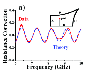
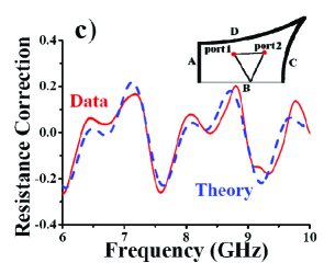
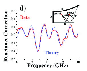
Figure 1: (Color online) Plot of corrections to the impedance due to (a) one-port with one wall (wall B), (b) one-port with two walls (walls C and D), (c) two-port with one wall (wall B), and (d) two-port with two walls (walls B and C) short trajectories, versus frequency from 6 to 10 GHz inside the $1/4$-bow-tie cavity. Shown are the theoretical predictions ($\textrm{Re}[z_{cor}^{(L_{M})}]$ and $\textrm{Im}[z_{cor}^{(L_{M})}]$) in blue (dashed) curves and experimental data ($\textrm{Re}[z_{cor}]$ and $\textrm{Im}[z_{cor}]$) in red (solid) curves.
The insets show the $1/4$-bow-tie billiard with thicker lines representing walls covered by microwave absorbers, the ports are shown as circular dots, and a few short trajectories are represented with lines as illustrations.

Fig. 1 shows comparisons between the measured impedance ($Z_{W}$) and the theoretical form ($Z^{(L_{M})}_{W}$). Here the impedance $Z_{W}$ is measured from the microwave cavity with specific walls ($W$) exposed, where $W=B$, $CD$, or $BC$ stands for one or more of the walls A, B, C, and D shown in the insets of Fig. 1. We have examined different combinations of exposed walls and choose some representative cases to show here. Figs. 1 (a) and (b) are for the cases of one-port experiments with (a) one wall exposed (wall B) and (b) two walls exposed (walls C and D), and Figs. 1 (c) and (d) are for cases of two-port experiments with (c) one wall exposed (wall B) and (d) two walls exposed (walls B and C). Notice that $Z_{avg}^{(L_{M})}\rightarrow Z^{(L_{M})}_{W}$ in this case because there is only one single realization. Thus, there is no ensemble averaging and $p_{b(n,m)}=1$ for all trajectories in Eqs. (7) and (8).

Here we focus on the effects of ray trajectories, so we remove the effect of the port mismatch from the measured impedance. We term this quantity the impedance correction

$$z_{cor}\equiv R_{R}^{-1/2}(Z_{W}-Z_{R})R_{R}^{-1/2},$$ (12)

and in Fig. 1 the measured data (red and solid) are constructed as the resistance correction $\textrm{Re}[z_{cor}]$ and the reactance correction $\textrm{Im}[z_{cor}]$. In each case, the radiation impedance of the antenna ($Z_{R}$) is determined by a separate measurement in which all four walls are covered by the microwave absorbers S1 . According to Eq. (2), the corresponding theoretical term is

$$z_{cor}^{(L_{M})}\equiv R_{R}^{-1/2}(Z^{(L_{M})}_{W}-Z_{R})R_{R}^{-1/2}$$

$$\ \ \ \ \ \ =\rho^{(L_{M})}_{W}+i\chi^{(L_{M})}_{W}=z^{(L_{M})}_{W}.$$ (13)

Therefore, the theoretical curves (blue dashed) of the resistance correction and the reactance correction in Fig. 1 are $\textrm{Re}[z_{cor}^{(L_{M})}]$ and $\textrm{Im}[z_{cor}^{(L_{M})}]$, respectively, and they can be calculated by using Eq. (6) with the known geometry of the cavity and port locations, including all short orbits up to the maximum length $L_{M}=200$ cm.

The measured data generally follow the theoretical predictions quite well, thus verifying that the theory offers a quantitative prediction of short-trajectory features of the impedance $Z_{W}$. In Figs. 1 (a) and (b), the one-port cases, we examine the resistance (reactance) correction for the waves entering and returning from the cavity through the single port, and the short-trajectory corrections respectively include one trajectory for $W=B$ and a sum over nine trajectories for $W=CD$. In Figs. 1 (c) and (d), the two-port cases, we examine the resistance (reactance) correction between the two ports. It corresponds to the elements $z_{cor,1,2}$ and $z_{cor,1,2}^{(L_{M})}$ in the $2\times 2$ matrices ($z_{cor}$ and $z_{cor}^{(L_{M})}$), and the short-trajectory corrections respectively include sums over two trajectories $(W=B)$ and four trajectories $(W=BC)$. For illustration, the insets of Fig. 1 show some representative short ray trajectories. Note the direct trajectory between the two ports without bouncing on walls is treated as a ray trajectory in Eqs. (7) and (8).

For the propagation attenuation, a frequency-dependent attenuation parameter $\kappa(f)$ is calculated utilizing the previously measured frequency-dependent loss parameter $\alpha$ SamThesis for this cavity. Fig. 2 shows the loss parameter $\alpha(f)$ and the attenuation parameter $\kappa(f)$ for the empty cavity case. Here $\alpha$ is defined as the ratio of the closed-cavity mode resonance 3-dB bandwidth to the mean spacing between cavity modes, $\alpha=k^{2}/(\Delta k^{2}Q)\simeq k^{2}A/(4\pi Q)$, where $A$ is the area of the cavity ($A=0.115m^{2}$), $k$ is the wavenumber, and $Q$ is the quality factor of the cavity. The mean spacing between modes varies from 21 MHz at 6 GHz to 6.9 MHz at 18 GHz. We obtain the loss parameter $\alpha$ from the measured impedance data in the empty cavity case according to the procedures presented in previous work S1 ; S3 ; SamThesis . In this procedure the frequency-dependent loss parameter $\alpha(f)$ is determined by selecting a proper frequency range (e.g., 1.8 GHz), computing the PDF of the “perfectly coupled” normalized impedance $i\xi_{0}$ (Eq. (1)), and then comparing to different PDFs that were generated from numerical RMT, using $\alpha$ as a fitting parameter. Once $\alpha(f)$ is known, the frequency-dependent attenuation parameter $\kappa(f)$ can be calculated because the dominant attenuation comes from losses in the top and bottom plates of the cavity, and it is well modeled by assuming that the waves suffer a spatially uniform propagation loss $\kappa=k/(2Q)=2\pi\alpha/(kA)$.

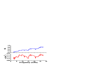
Figure 2: (Color online) Plot of the loss parameter $\alpha$ and the attenuation parameter $\kappa$ versus frequency inside the empty $1/4$-bow-tie cavity.

IV.2 Sources of errors

We propose that there are two major sources of the deviations between the theory and experiment shown in Fig. 1. The first is that the microwave absorbers do not fully suppress the trajectories, and the second arises from the ends of microwave absorbers that scatter energy back to the ports. To verify this, the $k=\omega/c$ dependent impedance corrections data in Fig. 1 are Fourier transformed to the length domain and shown in Fig. 3 as $\varepsilon(L)_{meas}\equiv c|\textrm{FT}\{z_{cor}\}|$ and $\varepsilon(L)_{theory}\equiv c|\textrm{FT}\{z_{cor}^{(L_{M})}\}|$, where $c$ is the speed of light, and $\textrm{FT}\{...\}$ is the Fourier transformation ($k\rightarrow L$). Note that the frequency range of the Fourier transformation is from 6 GHz to 18 GHz, and therefore, the resolution in length is 2.5 cm.

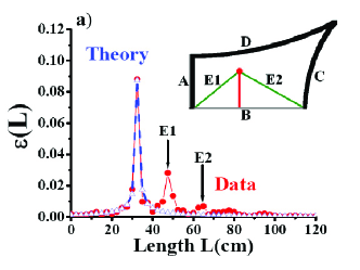
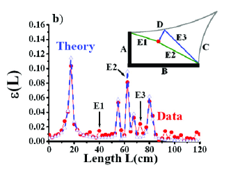
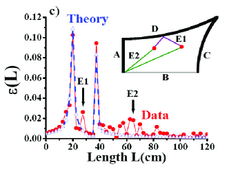
Figure 3: (Color online) Plot of the absolute values of the impedance correction in the length domain $\varepsilon(L)$ in the cases of (a) one-port with one wall (wall B), (b) one-port with two walls (walls C and D), (c) two-port with one wall (wall B), and (d) two-port with two walls (walls B and C) short trajectories, versus length from 0 to 120 cm inside the $1/4$-bow-tie cavity. Shown are the measured data in red curves with circular symbols and the theory in blue dashed curves with triangular symbols. The insets show the $1/4$-bow-tie billiard with labeled trajectories that show the sources of error (E1, E2, and E3).

In the length domain, the major peaks of the measured data (red) match the peaks of the theoretical prediction (blue and dashed), and this verifies that the short-trajectory correction can describe the major features of the measured impedance in the scattering system. For example, the matched peak in the theory curve and the data curve in Fig. 3(a) corresponds to the short trajectory from the port to wall B and returning, shown as the red (vertical) line in the inset of 3(a). However, there are several minor peaks in the measured data not present in the theoretical curves. After further examination of the geometry, the positions of these deviations in Fig. 3 match the lengths of trajectories which are related to the partially-blocked corners of the cavity, or bounce off microwave absorbers with a large incident angle. When the microwave absorbers end at the corners, they produce gaps and edges, and these defects create weak diffractive short trajectories. For example, the green lines E1 and E2 in the insets in Figs. 3(a) and (b) and E2 in Figs. 3(c) and (d) represent the diffractive short trajectories leaving a port, bouncing off the partially covered corners, and returning to a port. Their path lengths match the deviations between the measured data and the theory as labeled in the figure. Furthermore, the blue line E3 in the inset in Fig. 3(b) represents the short trajectories produced by the corner and bounced from one wall.

The other source of error is imperfection of the microwave absorbers that reflect $\sim-20$ dB of the incident signal for normal incidence, and more for oblique incidence. Therefore the short trajectories shown as purple lines E1 in Figs. 3(c) and (d) with a large incident angle bring about deviations between the theory and experimental data. These sources of error due to the ends of absorbers or large incident angles on absorbers were not included in the short-trajectory correction. However, these errors will not concern us further because all microwave absorbers are removed from the cavity in the experiments discussed below.

Besides the errors discussed above, another source of error is the difficulty in reproducing the antenna geometry with each measurement as the cavity is opened and re-sealed between the measurement of the radiation impedance and exposed wall cases. Another concern is multiply-reflected trajectories that bounce off of the antennas. However, because we describe trajectories in terms of the impedance instead of the scattering parameter, the multiply-reflected trajectories are incorporated in a single impedance term (see impedance ). This is an important advantage of using impedance because it can take account of the multiple-reflected trajectories in a simple compact form.

IV.3 Short-trajectory correction in the empty cavity

In the next experiment, an empty $1/4$-bow-tie cavity with no microwave absorbers or perturbers is used. Therefore, all possible trajectories between ports are present in this single realization. Fig. 4 shows (a) the real and (b) the imaginary parts of the first diagonal component of the impedance in a two-port cavity, corresponding to $\textrm{Re}[Z_{11}]$ and $\textrm{Im}[Z_{11}]$. Figs. 4 (c) and (d) are for the off-diagonal component of the impedance, $\textrm{Re}[Z_{12}]$ and $\textrm{Im}[Z_{12}]$. The radiation impedance (black) traces through the center of the fluctuating impedance data of the empty cavity and represents the nonuniversal aspects of the coupling antennas Henry_paper_one_port ; Henry_paper_many_port ; S1 . Note for the $Z_{12}$ case, all signals from port 1 to port 2 are treated as trajectories, so the off-diagonal radiation impedance is zero. Also shown in Fig. 4, the theoretical impedance $Z^{(L_{M})}$ (Eqs. (7) and (8)) include a finite number of short trajectories ($L_{M}=200$ cm, given a total of 584 trajectories for $Z^{(L_{M})}_{11}$ and 1088 trajectories for $Z^{(L_{M})}_{12}$). Note that the attenuation parameter $\kappa(f)$ is determined through the same procedures as in Sec. IV.1.

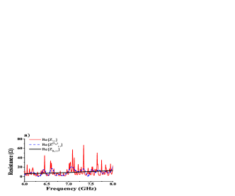
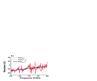
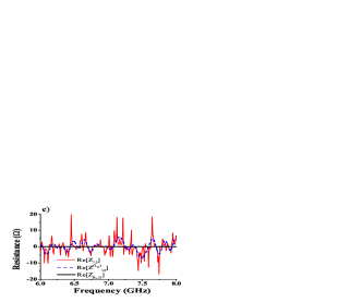
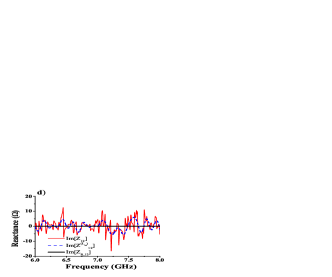
Figure 4: (Color online) Plot of the impedance due to the trajectories of four side-walls, versus frequency from 6 to 8 GHz inside the empty $1/4$-bow-tie cavity. Shown are (a) the real part of $Z_{11}$, (b) the imaginary part of $Z_{11}$, (c) the real part of $Z_{12}$ and (d) the imaginary part of $Z_{12}$. The three curves are the measured impedance $Z$ (red thinner), the theoretical impedance $Z^{(L_{M})}$ (blue dashed), as well as the radiation impedance $Z_{R}$ (black).

In Fig. 4, the theoretical impedance $Z^{(L_{M})}$ tracks the main features of the single-realization measured impedance although there are many sharp deviations between the two sets of curves. These fluctuations are expected because of the infinite number of trajectories ($L_{b(n,m)}>200$ cm) not included in the theory.

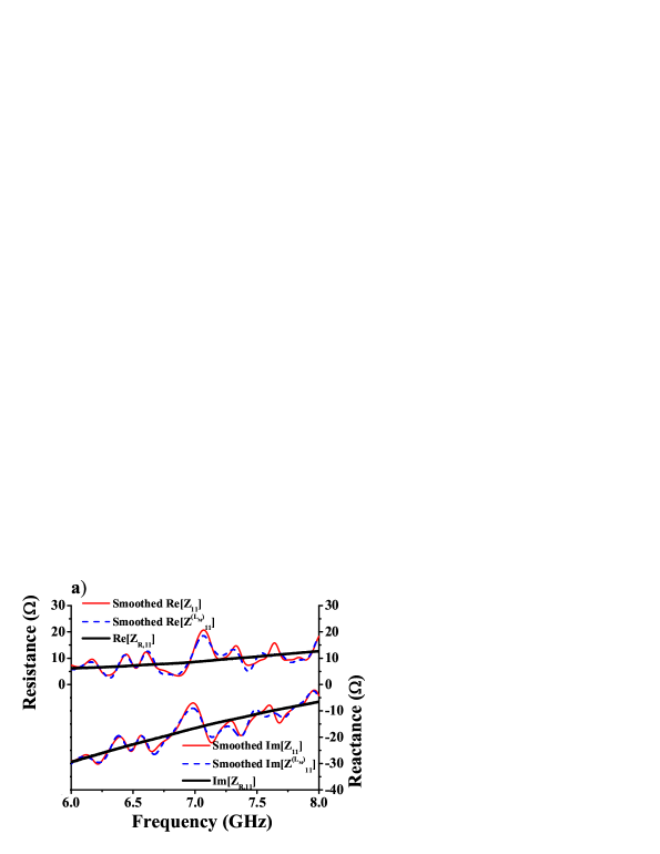
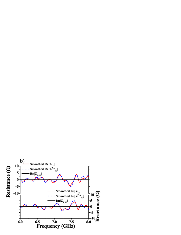
Figure 5: (Color online) Plot of the smoothed impedance versus frequency from 6 to 8 GHz. Shown are, (a) for $Z_{11}$ and (b) for $Z_{12}$, the real (three upper curves) and the imaginary part (three lower curves) of the smoothed impedance for the theory ($Z^{(L_{M})}$ with $L_{M}=200$ cm, blue dashed) and the experiment (red solid), as well as the measured (un-smoothed) radiation impedance of the port ($Z_{R}$, black thick).

It is more appropriate to compare the theory to a frequency ensemble of single-realization data. A frequency ensemble is created by considering frequency smoothed experimental data and comparing it with the smoothed theoretical prediction for system-specific contributions to the impedance. The frequency smoothing (Eqs. (9) and (10)) suppresses the impedance fluctuations due to long trajectories and reveals the features associated with short trajectories. Fig. 5 shows the radiation impedance (black thick), the smoothed measured impedance $Z$ (red solid) and the smoothed theoretical impedance $Z^{(L_{M})}$ (blue dashed). The smoothing is made by a Gaussian smoothing function with the standard deviation $\Delta\omega/(2\pi)=240$ MHz (Eq. (10)). Gaussian frequency smoothing inserts an effective low-pass Gaussian filter on the trajectory length, and thus, the components of impedances ($Z$ and $Z^{(L_{M})}$) in the length domain are limited to those with the path length $L\lesssim 2\pi c/\Delta\omega=125$ cm. Fig. 5 shows that the smoothed theory matches the similarly smoothed experimental data very well, therefore, the short trajectory theory correctly captures the effects of ray trajectories out to this length region ($\lesssim 125$ cm).

When computing the sum of short-trajectory correction terms in a low loss case like the empty cavity, a problem appears associated with the finite number of terms ($L_{b(n,m)}\leq L_{M}$) in the sum over trajectories. In the theory, to perfectly reproduce the measured data in the empty cavity requires an infinite number of correction terms. Therefore, in some frequency regions where the experimental impedance changes rapidly, the finite sum for the theoretical resistance $\textrm{Re}[Z^{(L_{M})}]$ will show values less than zero, which are not physical for a passive system. For example, see the blue dashed curve in Fig. 4(a) between 7.3 and 7.4 GHz. This problem is similar to Gibbs phenomenon in which the sum of a finite number of terms of the Fourier series has large overshoots near a jump discontinuity.

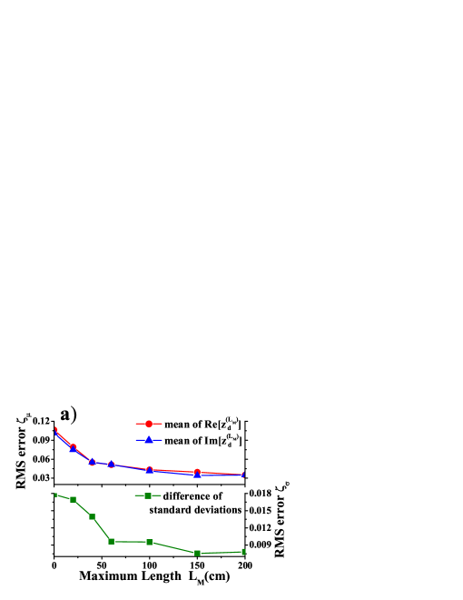
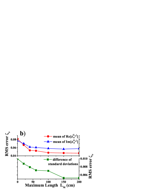
Figure 6: (Color online) Plot of the RMS errors for (a) the one-port experiment and (b) the two-port experiment. Shown are $\zeta_{\mu}$ for the mean of the real part (red circles) and the imaginary part (blue triangles) of the normalized impedance difference and $\zeta_{\sigma}$ for the difference of standard deviations (green rectangles), versus short-trajectory corrections with the maximum length from 0 to 200 cm. Data are taken for a single realization of the bow-tie cavity.

Besides verifying that the short-trajectory correction agrees with system-specific features of the measured data, we would next like to demonstrate that including short-trajectory corrections improves the ability to reveal underlying universal statistical properties, even in a single realization of the system. We compute the statistical properties of the real and imaginary part of the normalized impedance difference

$$z^{(L_{M})}_{d}\equiv R_{R}^{-1/2}(Z-Z^{(L_{M})})R_{R}^{-1/2}$$ (14)

in 500 MHz frequency windows from 6 to 18 GHz for a single realization of the bow-tie cavity. Random matrix theory predicts that the distribution of $\textrm{Re}[z^{(L_{M})}_{d}]$ and $\textrm{Im}[z^{(L_{M})}_{d}]$ should have zero means, and identical standard deviations Fyodorov ; S1 ; S2 ; S3 ; henrythesis ; Experimental_tests_our_work . For the one-port case, we use the normalized impedance difference value directly, and for the two-port case, we consider the eigenvalues of the $2\times 2$ normalized impedance difference matrix.

Fig. 6 shows that the RMS errors of statistical parameters between the measured data and the theory decrease upon including more short trajectories in the correction (i.e., increasing $L_{M}$). We compute the root mean square value of errors ($\zeta$ defined later) for a series of frequency windows covering the range from 6 to 18 GHz, and the results are shown versus different short-trajectory corrections with varied maximum lengths $L_{M}$. Notice the cases of $L_{M}=0$ denote the impedance corrected by only the radiation impedance without any short-trajectory correction. For the normalized impedance difference $z_{d}^{(L_{M})}$ in each frequency window, the RMS error $\zeta_{\mu}$ is defined as the root mean square value of $|\mu_{R}-0|$ or $|\mu_{X}-0|$ for the difference of the measured mean from zero, and $\zeta_{\sigma}$ is defined as the root mean square value of $|\sigma_{R}-\sigma_{X}|/(\sigma_{R}+\sigma_{X})$ for the difference of standard deviations between the real part PDF and the imaginary part PDF. Here $\mu_{R}$ and $\mu_{X}$ are respectively the means of $\textrm{Re}[z^{(L_{M})}_{d}]$ and $\textrm{Im}[z^{(L_{M})}_{d}]$ in each window, and $\sigma_{R}$ and $\sigma_{X}$ are the standard deviations of $\textrm{Re}[z^{(L_{M})}_{d}]$ and $\textrm{Im}[z^{(L_{M})}_{d}]$ in each window. In all three statistical parameters for both one-port and two-port cases, the RMS errors $\zeta$ decrease when we correct the data with more short trajectories. This verifies that using short-trajectory corrections in a single realization of the wave-chaotic system can more effectively reveal the universal statistical properties in the data.

IV.4 Configuration averaging approach

Many efforts to determine universal RMT statistics in experimental systems are based on a configuration averaging approach that creates an ensemble average from realizations with varied configurations. In principle, one can recover the nonuniversal properties of the system Brouwer_Lorentzian ; Kuhl via the configuration averaging approach, which is motivated by the “Poisson kernel” theory of Mello, Pereyra, and Seligman Poisson_Kernel_Original . Specifically, ensemble averages of the measured cavity data are used to remove the system-specific features in each single realization. Note that in the past, the configuration averaging approach was explicitly assumed to only remove the effects of the nonuniversal coupling; however, it was recently generalized to include the nonuniversal contributions of short trajectories Bulgakov_Gopar_Mello_Rotter .

Here the experimental results verify that the short-trajectory correction (Eqs. (7) and (8)) can describe nonuniversal characteristics of wave-chaotic systems in the configuration ensemble. Two cylindrical pieces of metal are added as perturbers in the wave-chaotic system that is shown in the inset of Fig. 7, where the dots represent the ports and the two circles represent the perturbers. The locations of the two perturbers inside the cavity are systematically changed and accurately recorded to produce a set of 100 realizations for the ensemble S2 ; S3 ; Experimental_tests_our_work . The scattering matrix $S$ is measured from 6 to 18 GHz, covering roughly 1070 modes of the closed cavity. After the ensemble average, longer ray trajectories have higher probability of being blocked by the two perturbers in the 100 realizations; therefore, the main nonuniversal contributions are due to shorter ray trajectories. We compare the measured ensemble averaged impedance $\langle Z\rangle$ and the theoretical impedance $Z_{avg}^{(L_{M})}$ that is calculated from Eqs. (7) and (8) with the maximum trajectory length $L_{M}=200$ cm.

In the configuration ensemble, contrary to the previous cases without perturbers, we need to introduce a survival probability $p_{b(n,m)}$ for each ray trajectory term in Eqs. (7) and (8). Notice that the two perturbers can block ray trajectories and influence their presence in the ensemble realizations. Thus, we multiply each term in the sum by a weight $p_{b(n,m)}$ equal to the fraction of perturbation configurations in which the trajectory is not intercepted by the perturbers. The values of $p_{b(n,m)}$ are between 0 and 1, and a longer ray trajectory generally has a higher chance of being blocked by perturbers, and thus it has smaller $p_{b(n,m)}$.

Note that by recording the positions of perturbers in all realizations, we are able to do impedance normalization with short-trajectory correction individually for each realization, similar to the procedures in the empty cavity case. Here we introduce $p_{b(n,m)}$ as a more general description for the case in which only the probabilities of survival of particular short trajectories are known. In addition, we ignore the effect of newly created trajectories by the perturbers in each specific realization because they are averaged out in the ensemble. Note that the attenuation parameter $\kappa$ in the short-trajectory correction terms (Eqs. (7) and (8)) is recalculated using the measured PDFs of impedance in the ensemble case, using procedures similar to those for the case of the empty cavity. Due to the presence of two perturbers in the cavity, the attenuation parameter and loss parameter are slightly larger ($\sim 0.1$ for $\alpha$) than in the empty cavity case.

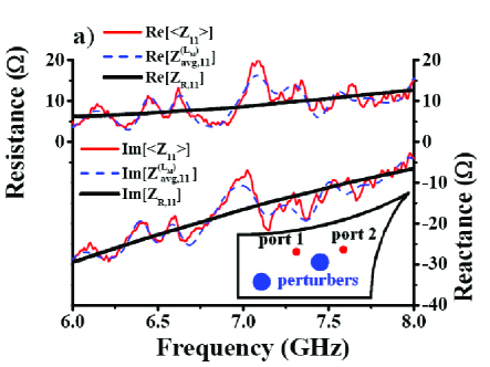
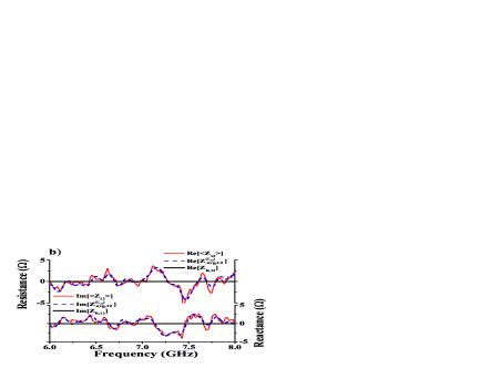
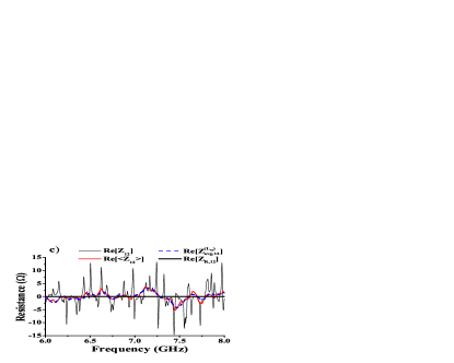
Figure 7: (Color online) Plot of the average impedance versus frequency from 6 to 8 GHz. Shown are, (a) for $Z_{11}$ and (b) for $Z_{12}$, the real (three upper curves) and the imaginary part (three lower curves) of the average impedance for the theory ($Z^{(L_{M})}_{avg}$ with $L_{M}=200$ cm, blue dashed) and the configuration average experiment ($\langle Z\rangle$ red solid), as well as the measured radiation impedance of the ports ($Z_{R}$, black thick). Plot (c) shows the real part of the measured impedance $Z_{12}$ (black thin) in a single realization comparing with $Z^{(L_{M})}_{avg,12}$ and $\langle Z_{12}\rangle$. Inset: The wave-chaotic two-dimensional cavity with perturbers and two ports.

The result of comparisons between the $2\times 2$ matrices $\langle Z\rangle$ and $Z^{(L_{M})}_{avg}$ of the two-port experiment is shown in Fig. 7. We have published the result of the one-port experiment in another paper Jenhao . Here Fig. 7 (a) shows the comparison of the first diagonal component of the impedance, and Fig. 7 (b) shows the comparison of the off-diagonal component. The measured data (red solid) follow the trend of the radiation impedance (black thick), and the theory (blue dashed) reproduces most of the fluctuations in the data by including only a modest number of short-trajectory correction terms. Fig. 7(c) illustrates the comparison between the measured impedance $Z$ in a single realization and $\langle Z\rangle$ The strong fluctuations in the measured impedance $Z$ (black thin) curve have diminished due to the configuration averaging, and the remaining fluctuations of the configuration averaged impedance $\langle Z\rangle$ away from the radiation impedance are closely tracked by the theoretical (blue dashed) curve. Note that no wavelength averaging is used here. The good agreement between the measured data and the theoretical prediction verifies that the new theory, Eqs. (7) and (8), predicts the nonuniversal features embodied in the ensemble averaged impedance well.

The deviations between the $\langle Z\rangle$ curves and the $Z^{(L_{M})}_{avg}$ curves in Fig. 7 may come from several effects. The first is the remaining fluctuations in the $\langle Z\rangle$ due to the finite number of realizations. We estimate this to be on the order of $\sigma_{\langle Z\rangle}\simeq\sigma_{Z}/\sqrt{100}\sim 1\Omega$, where $\sigma_{\langle Z\rangle}$ is the standard deviation of ensemble averaged impedance $\langle Z\rangle$ of 100 realizations, and $\sigma_{Z}$ is the standard deviation of the measured impedance $Z$ of a single realization. This accounts for the remaining sharp features in $\langle Z\rangle$. Another source of errors is that we ignore the effect of newly created trajectories by the perturbers. Even though these new trajectory terms are divided by 100 (the number of realizations), the remaining effects create small deviations.

We have demonstrated that the ensemble average technique reveals the nonuniversal properties of the system, and short-trajectory corrections can help to better describe the nonuniversal part than using the radiation impedance alone. Now we demonstrate the benefit of using the short-trajectory correction in another respect. That is, when removing the nonuniversal part to reveal the universal properties, the revealed universal properties have better agreement with the prediction of RMT if we take account of the short-trajectory correction. We compare the probability distribution of the eigenvalues of the normalized impedance $i\xi_{0}$ [normalized by the radiation impedance (see Eq. (1))], $i\xi^{(L_{M})}$ [normalized by the short-trajectory-corrected impedance (see Eq. (3))], and the PDFs that were generated from numerical RMT S1 ; S3 ; SamThesis .

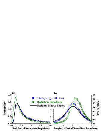
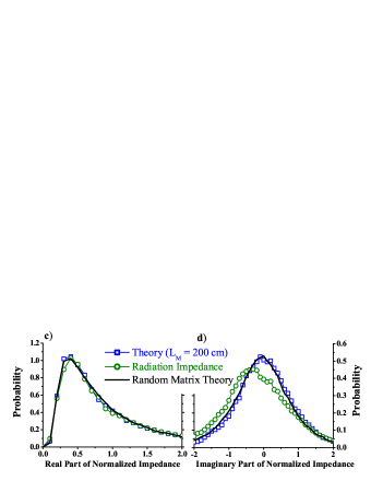
Figure 8: (Color online) Plot of probability distributions of (a) the real part and (b) the imaginary part of the normalized impedance eigenvalues in the frequency range 6.8 GHz $\sim$ 7.0 GHz, and (c) the real part and (d) the imaginary part of the normalized impedance in the frequency range 11.0 GHz $\sim$ 11.2 GHz. The blue (squares) curve is $i\xi^{(L_{M})}$ that is normalized with the short-trajectory-corrected impedance, the green (circles) curve is $i\xi_{0}$ that is normalized with the radiation impedance only, and the black curve shows the PDF generated from numerical RMT.

Fig. 8 shows the PDFs of the normalized impedance $i\xi_{0}$, $i\xi^{(L_{M})}$, and the corresponding data from numerical RMT. For $i\xi_{0}$ in Eq. (1), we take the impedance $Z$ from the 100 realizations and in a frequency range of 200 MHz. Similarly, for $i\xi^{(L_{M})}$ in Eq. (3), we use the same measured data but consider short-trajectory correction with $L_{M}=200$ cm in addition to the radiation impedance. Here we show two examples for frequency ranges 6.8 GHz $\sim$ 7.0 GHz in Figs. 8 (a) and (b); and 11.0 GHz $\sim$ 11.2 GHz in Figs. 8 (c) and (d). It should be noted that in the past such narrow frequency ranges were not used because short trajectories created strong deviations from RMT predictions S1 ; S2 ; S3 . Because the normalized impedance is complex, Figs. 8 (a) and (c) show the distribution of the real part of the normalized impedance; (b) and (d) are the imaginary part. For the numerical RMT data, the loss parameters ($\alpha=0.3$ for 6.8 GHz $\sim$ 7.0 GHz and $\alpha=0.4$ for 11.0 GHz $\sim$ 11.2 GHz) were determined by the best matched distribution with a much wider frequency range (2 GHz). As seen in Fig. 8 the distribution of the normalized impedance has much better agreement with the prediction of RMT when we consider the short-trajectory correction up to the trajectory length of 200 cm.

The deviations of the distribution between the normalized impedance and the predictions of RMT in Fig. 8 are due to short trajectories that remain in the ensemble average of the 100 realizations. We have seen that the PDFs of $i\xi_{0}$ and $i\xi^{(L_{M})}$ approach each other when we use the data in a wider frequency range. This is because in a wide enough frequency window the fluctuations in the impedance due to a trajectory can be compensated (i.e., the required window is 1.8 (GHz) $\simeq c/17$(cm) for the shortest trajectory with $L_{b(1,1)}=15$ cm and $L_{port(1,1)}=2$ cm). Therefore, we take a 2 GHz frequency window to obtain a universal distribution that is independent of which normalization methods we use (Eq. (1) or Eq. (3)), and we also determine the loss parameter from this universal distribution S1 ; S3 ; SamThesis .

Furthermore, the deviations shown in Fig. 8 match the difference between $\langle Z\rangle$ and $Z_{R}$ shown in Fig. 7. For example, in the frequency range 6.8 GHz $\sim$ 7.0 GHz the ensemble averaged impedance $\langle Z_{11}\rangle$ is smaller than the radiation impedance $Z_{R,11}$ in the real part and larger in the imaginary part, and in Figs. 8 (a) and (b) we can see the same bias of the distribution of the normalized impedance $i\xi_{0}$ that is normalized with the radiation impedance only. Therefore, with short-trajectory corrections, we can better explain the deviations between the measured ensemble average and the universal properties predicted by RMT.

IV.5 Uncovering RMT statistics of the scattering matrix

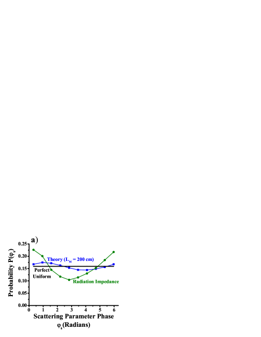
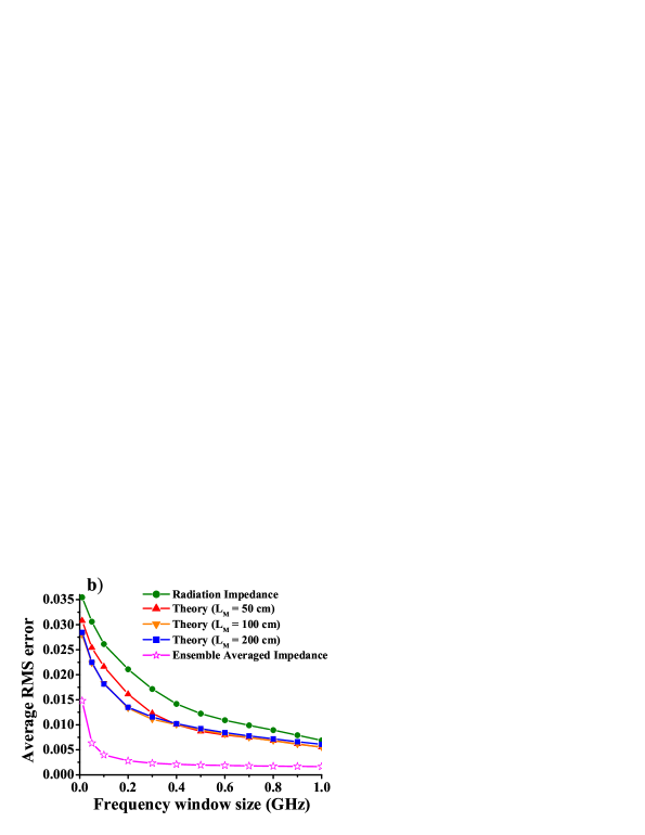
Figure 9: (Color online) Plot of (a) an example probability distribution of the phase $\varphi_{s}$ of eigenvalues of the normalized scattering matrix $s^{(L_{M})}$ from $0\sim 2\pi$, taken over the 11$\sim$11.5 GHz frequency window inside the $1/4$-bow-tie cavity of 100 realizations with perturbers. The blue (squares) curve is from data normalized with $L_{M}=200$ cm, the green (circles) curve is from data normalized with the radiation impedance only, and the black line shows the perfectly uniform distribution for comparison. Plot of (b) the average RMS error of distributions of $\varphi_{s}$, where the normalized scattering matrix $s^{(L_{M})}$ is calculated from impedance normalized with the radiation impedance only (green circles), with the measured ensemble averaged impedance (pink stars), or with theoretical impedance with $L_{M}=50$ cm (red triangles), 100 cm (orange invert triangles), up to 200 cm (blue squares), versus frequency window size from 10 MHz to 1.0 GHz.

We now test the benefits of the short-trajectory correction in uncovering universal RMT statistics of the scattering matrix. We find that including short trajectories in the impedance normalization improves our determination of the RMT statistical properties of the scattering matrix $S$, given the same amount of ensemble and frequency averaging. In other words, we show that the need to resort to wavelength averaging over large numbers of modes is significantly reduced after including short-trajectory corrections in the impedance normalization. This section shows the result of the two-port experiment; the result of the one-port experiment has been published in our previous work Jenhao . Here we examine the phase $\varphi_{s}$ of the eigenvalues of the normalized scattering matrix $s^{(L_{M})}$ because the statistics of $\varphi_{s}$ do not change with the frequency-dependent loss parameter $\alpha(f)$ S3 . The normalized scattering matrix $s^{(L_{M})}$ is defined as $(i\xi^{(L_{M})}-1)/(i\xi^{(L_{M})}+1)=|s^{(L_{M})}|e^{i\varphi_{s}}$, where the normalized impedance $i\xi^{(L_{M})}$ is given by Eq. (3) with corrections by Eqs. (7) and (8). Note for the two-port experiment, we compute the eigenvalues of the matrix $s^{(L_{M})}$, and $\varphi_{s}$ is the phase of the eigenvalues. RMT predicts that $\varphi_{s}$ should have a uniform distribution from 0 to $2\pi$ independent of loss Poisson_Kernel_Original ; Brouwer_Lorentzian , as verified in previous experiments S2 ; S3 .

Fig. 9 illustrates the benefits of using short-trajectory-corrected data to examine the statistical properties of the scattering matrix. An ensemble of data is created by averaging 100 realizations of the cavity with the two perturbers present, between 6 and 18 GHz, encompassing about 1070 closed-cavity modes. Theoretical short trajectory corrections are weighted by the survival probability ($p_{b(n,m)}$) which are calculated from the known locations of the perturbers. Fig. 9(a) shows a representative probability distribution ($P(\varphi_{s})$) of the phase of eigenvalues of the normalized scattering matrix. The data for the normalized scattering matrix are formed by taking the measured impedance from each of the 100 realizations and normalizing with the radiation impedances $Z_{R}$ or the theoretical impedance with short-trajectory correction $Z_{avg}^{L_{M}}$, and these PDFs are computed from the data in a 500 MHz frequency range ($11.0\sim 11.5$ GHz). In this frequency range, it is clear that the distribution normalized with short trajectories is significantly closer to a uniform distribution than the one normalized without short trajectories.

To quantify this improvement, it is convenient to look at the average root-mean-square (RMS) error with respect to the uniform distribution for the two types of normalization (Fig. 9(b)). Here the RMS error is defined as

$$RMS\ error\equiv\sqrt{\frac{1}{10}\sum_{i=1}^{10}\left(\frac{n_{i}}{\langle n_{i}\rangle}-1\right)^{2}},$$ (15)

where $n_{i}$ is the number of elements in the $i^{th}$ bin in the 10 bins histogram of $P(\varphi_{s})$, and $\langle n_{i}\rangle$ is the mean of $n_{i}$. Therefore, when a distribution is more uniform, its RMS error is smaller. The average RMS error of each frequency window is averaged over the spectral range from 6 to 18 GHz, and Fig. 9(b) shows the average RMS error versus the frequency window sizes from 10 MHz to 1.0 GHz. This figure shows that the distributions of data are systematically more uniform as more short trajectories are taken into account in the normalization for a given window size. The average RMS error of the data normalized without short trajectories (the radiation impedance only (green circles)) has the largest error. When we include more short trajectories from the maximum lengths $L_{M}=50$ cm (red triangles) up to $L_{M}=200$ cm (blue squares), the average RMS errors decrease. The improvement is obvious after including short trajectories with $L_{M}=50$ cm, and it saturates for trajectories with $L_{M}=100$ cm. For comparison, we also add a curve (pink stars) for the data normalized by the measured ensemble averaged impedance $\langle Z\rangle$ (the red curves in Fig. 7), and it is the most uniform case. It is observed that the improvement of statistical properties with short-trajectory corrections is more significant when the frequency window size is smaller.

V Conclusions

A theory for the nonuniversal effects of coupling and short ray trajectories on scattering wave-chaotic systems has been tested experimentally on a two-dimensional, wave-chaotic, electromagnetic cavity with one or two transmission line channels connecting to the outside. In particular, the theoretical predictions match the measured data in the cases of a frequency ensemble in a single realization and the configuration ensemble in the ensemble of 100 realizations. By removing nonuniversal effects from measured data, we can reveal underlying universally fluctuating quantities in the scattering and impedance matrices. These results should be useful in many fields where similar wave phenomena are of interest, such as nuclear scattering, atomic physics, quantum transport in condensed matter systems, electromagnetics, acoustics, geophysics, etc.

References

- (1) J. Verbaarschot, H. Weidenmüller, and M. R. Zirnbauer, Phys. Rep. 129, 367 (1985).
- (2) M. L. Mehta, Random Matrices (Academic Press, San Diego, 1991).
- (3) C.W.J. Beenakker, Rev. Mod. Phys. 69, 731 (1997).
- (4) H. J. Stöckmann, Quantum Chaos (Cambridge University Press, New York, 1999).
- (5) Y. V. Fyodorov, D. V. Savin, and H.-J Sommers, J. Phys. A 38, 10731 (2005).
- (6) S. Hemmady, X. Zheng, E. Ott, T. M. Antonsen, and S. M. Anlage, Phys. Rev. Lett. 94, 014102 (2005).
- (7) P. A. Mello, P. Pereyra, and T. H. Seligman, Ann. Phys. 161, 254 (1985).
- (8) P. W. Brouwer, Phys. Rev. B 51, 16878 (1995).
- (9) H. U. Baranger and P. A. Mello, Europhys. Lett. 33, 465 (1996).
- (10) K. Richter and M. Sieber, Phys. Rev. Lett. 89, 206801 (2002).
- (11) U. Kuhl, M. Martínez-Mares, R. A. Méndez-Sánchez, and H.-J. Stöckmann, Phys. Rev. Lett. 94, 144101 (2005).
- (12) X. Zheng, T. M. Antonsen, and E. Ott, Electromagnetics 26, 3 (2006).
- (13) X. Zheng, T. M. Antonsen, and E. Ott, Electromagnetics 26, 27 (2006).
- (14) S. Müller, S. Heusler, P. Braun, and F. Haake, New J. Phys. 9, 12 (2007).
- (15) R. Schäfer, T. Gorin, T. H. Seligman, and H.-J. Stöckmann, New J. Phys. 7, 152 (2005).
- (16) M. C. Gutzwiller, Chaos in Classical and Quantum Mechanics (Springer-Verlag, New York, 1990).
- (17) J. Stein and H.-J. Stöckmann, Phys. Rev. Lett. 68, 2867 (1992).
- (18) H. Ishio and J. Burgdörfer, Phys. Rev. B 51, 2013 (1995).
- (19) L. Wirtz, J.-Z. Tang, and J. Burgdörfer, Phys. Rev. B 56, 7589 (1997).
- (20) R. G. Nazmitdinov, K. N. Pichugin, I. Rotter, and P. Šeba, Phys. Rev. B 66, 085322 (2002).
- (21) H. Ishio and J. P. Keating, J. Phys. A 37, L217 (2004).
- (22) R. E. Prange, J. Phys. A 38, 10703 (2005).
- (23) C. Stampfer, S. Rotter, J. Burgdörfer, and L. Wirtz, Phys. Rev. E 72, 036223 (2005).
- (24) X. Zheng, S. Hemmady, T. M. Antonsen, S. M. Anlage, and E. Ott, Phys. Rev. E 73, 046208 (2006).
- (25) S. Hemmady, X. Zheng, J. Hart, T. M. Antonsen, E. Ott, and S. M. Anlage, Phys. Rev. E 74, 036213 (2006).
- (26) S. Hemmady, J. Hart, X. Zheng, T. M. Antonsen, E. Ott, and S. M. Anlage, Phys. Rev. B 74, 195326 (2006).
- (27) J. Hart, T. Antonsen, and E. Ott, Phys. Rev. E 80, 041109 (2009).
- (28) D. Wintgen and H. Friedrich, Phys. Rev. A 36, 131 (1987).
- (29) M. Sieber and K. Richter, Phys. Scr. T90, 128 (2001).
- (30) J. D. Urbina and K. Richter, Phys. Rev. E 70, 015201 (2004).
- (31) J. D. Urbina and K. Richter, Phys. Rev. Lett. 97, 214101 (2006).
- (32) T. Kottos and U. Smilansky, J. Phys. A 36, 3501 (2003).
- (33) E. N. Bulgakov, V. A. Gopar, P. A. Mello, and I. Rotter, Phys. Rev. B 73, 155302 (2006).
- (34) J.-H. Yeh, J. A. Hart, E. Bradshaw, T. M. Antonsen, E. Ott, and S. M. Anlage, Phys. Rev. E 81, 025201(R) (2010).
- (35) F. J. Dyson, J. Math. Phys. 3, 140 (1962).
- (36) E. Doron and U. Smilansky, Nucl. Phys. A 545, 455 (1992).
- (37) P. A. Mello and H. U. Baranger, Waves in Random Media 9, 105 (1999).
- (38) F. Beck, C. Dembowski, A. Heine, and A. Richter, Phys. Rev. E 67(6), 066208 (2003).
- (39) J. Barthélemy, O. Legrand, and F. Mortessagne, Phys. Rev. E 71, 016205 (2005).
- (40) J. Barthélemy, O. Legrand, and F. Mortessagne, Europhys. Lett. 70, 162 (2005).
- (41) B. Dietz, et al., Phys. Rev. E 78(5), 055204 (2008).
- (42) The impedance matrix gives the linear relation between the voltages at the ports and the currents. For the problem we consider, the ports are antennas that are much smaller than a wavelength and thus, have fixed current distributions. In this case, if the current at a port/antenna is specified, a wave incident on it from the interior will not be scattered. Thus, contributions to the voltage at that port, due to ray trajectories leading to that port, may be summed. Scattering of waves by the port/antenna occurs when the port current is allowed to respond to the port voltage, for example, if the port is connected to a transmission line with characteristic impedance . Note, the effect of multiple refections from the ports is included in the scattering matrix .
- (43) Y. Alhassid, Rev. Mod. Phys. 72, 895 (2000).
- (44) Y. V. Fyodorov and D. V. Savin, JETP Letters 80, 725 (2004).
- (45) D. V. Savin and H.-J. Sommers and Y. V. Fyodorov, JETP Letters 82, 544 (2005).
- (46) X. Zheng, Ph.D. thesis, University of Maryland (2005), http://hdl.handle.net/1903/2920.
- (47) S. Hemmady, X. Zheng, T. M. Antonsen, E. Ott, and S. M. Anlage, Phys. Rev. E 71, 056215 (2005).
- (48) A. Gokirmak, D. H. Wu, J. Bridgewater, and S. M. Anlage, Rev. Sci. Instrum. 69, 3410 (1998)
- (49) P. So, S. M. Anlage, E. Ott, and R. N. Oerter, Phys. Rev. Lett. 74, 2662 (1995).
- (50) S.-H. Chung, A. Gokirmak, D.-H. Wu, J. S. A. Bridgewater, E. Ott, T. M. Antonsen, and S. M. Anlage, Phys. Rev. Lett. 85, 2482 (2000).
- (51) S. Hemmady, Ph.D. Thesis, University of Maryland (2006), http://hdl.handle.net/1903/3979.