The Luminosity Function of Lyman alpha Emitters at Redshift $z=7.7$

Abstract

Lyman alpha ( Ly$\alpha\;$) emission lines should be attenuated in a neutral intergalactic medium (IGM). Therefore the visibility of Ly$\alpha\;$ emitters at high redshifts can serve as a valuable probe of reionization at about the 50$\%$ level. We present an imaging search for $z=7.7$ Ly$\alpha\;$ emitting galaxies using an ultra-narrowband filter (filter width=$\rm 9\AA$) on the NEWFIRM imager at the Kitt Peak National Observatory. We found four candidate Ly$\alpha\;$ emitters in a survey volume of $1.4\times 10^{4}\rm Mpc^{3}$, with a line flux brighter than $6\times 10^{-18}{\rm\,erg\,cm^{-2}\,s^{-1}}$ (5$\sigma$ in 2^′′ aperture). We also performed a detailed Monte-Carlo simulation incorporating the instrumental effects to estimate the expected number of Ly$\alpha\;$ emitters in our survey, and found that we should expect to detect one Ly$\alpha\;$ emitter, assuming a non-evolving Ly$\alpha\;$ luminosity function (LF) between $z$=6.5 and $z$=7.7. Even if one of the present candidates is spectroscopically confirmed as a $z\approx 8$ Ly$\alpha\;$ emitter, it would indicate that there is no significant evolution of the Ly$\alpha\;$ LF from $z=3.1$ to $z\approx 8$. While firm conclusions would need both spectroscopic confirmations and larger surveys to boost the number counts of galaxies, we successfully demonstrate the feasibility of sensitive near-infrared ($1.06\mu$m) narrow-band searches using custom filters designed to avoid the OH emission lines that make up most of the sky background.

1. Introduction

Lyman alpha ( Ly$\alpha\;$) emitting galaxies offer a powerful probe of both galaxy evolution and the reionization history of the universe. Ly$\alpha\;$ emission can be used as a prominent signpost for young galaxies whose continuum emission may be below usual detection thresholds. It is also a tool to study their star formation activity, and a handle for spectroscopic followup.

The intergalactic medium (IGM) will obscure Ly$\alpha\;$ emission from view if the neutral fraction exceeds $\sim 50\%$ (Furlanetto et al., 2006; McQuinn et al., 2007). Recently, Ly$\alpha\;$ emitters have been used to show that the IGM is $\lesssim 50\%$ neutral at $z=6.5$ (Rhoads & Malhotra, 2001; Malhotra & Rhoads, 2004; Stern et al., 2005; Kashikawa et al., 2006; Malhotra & Rhoads, 2006). This complements the Gunn-Peterson $lower$ bound of $x_{HI}\gtrsim 1\%$ at $z\approx 6.3$. Completely independently, polarization of the cosmic microwave bakground suggests a central reionization redshift $z_{re}=10.5\pm 1.2$ (Komatsu et al., 2010).

In addition to their utility as probes of reionization, Ly$\alpha\;$ emitters are valuable in understanding galaxy formation and evolution at the highest redshifts. This is especially true for low mass galaxies, as Ly$\alpha\;$ emitters are observed to have stellar masses $\rm M_{\star}\lesssim 10^{9}\;M_{\odot}$ (Gawiser et al., 2006; Pirzkal et al., 2007; Finkelstein et al., 2007; Pentericci et al., 2009), appreciably below the stellar masses of Lyman break selected galaxies (LBG) (Steidel et al., 1996) at similar redshifts (e.g. Papovich et al., 2001; Shapley et al., 2001; Stark et al., 2009).

Narrow-band imaging is a well established technique for finding high redshift galaxies (e.g. Rhoads, 2000a; Rhoads et al., 2004, 2003; Malhotra & Rhoads, 2002, 2004; Cowie & Hu, 1998; Hu et al., 1999, 2002, 2004; Kudritzki et al., 2000; Fynbo et al., 2001; Pentericci et al., 2000; Ouchi et al., 2001, 2003, 2008; Stiavelli et al., 2001; Shimasaku et al., 2006; Kodaira et al., 2003; Ajiki et al., 2004; Taniguchi et al., 2005; Venemans et al., 2004; Kashikawa et al., 2006; Iye et al., 2006; Nilsson et al., 2007; Finkelstein et al., 2009). The method works because Ly$\alpha\;$ emission redshifted into a narrow band filter will make the emitting galaxies appear brighter in images through that filter than in broadbands of similar wavelength. A supplemental requirement that the selected emission line galaxies be faint or undetected in filters blueward of the narrowband filter effectively weeds out lower redshift emission line objects (e.g. Malhotra & Rhoads, 2002). This has proven to be very efficient for selecting star-forming galaxies up to $z\lesssim 7$, and remains effective even when those galaxies are too faint in their continuum emission to be detected in typical broadband surveys.

While large samples of Ly$\alpha\;$ emitters have been detected at $z<$6, both survey volumes and sample sizes are much smaller at $z>$6. Since the Ly$\alpha\;$ photons are resonantly scattered in neutral IGM, a decline in the observed luminosity function (LF) of Ly$\alpha\;$ emitters would suggest a change in the IGM phase, assuming the number density of newly formed galaxies remains constant at each epoch. Malhotra & Rhoads (2004) found no significant evolution of Ly$\alpha\;$ LF between $z$=5.7 and $z$=6.6, while Kashikawa et al. (2006) suggested an evolution of bright end of the Ly$\alpha\;$ LF in this redshift range. At even higher redshifts, $z=6.5$ to $z$=7, some authors (Iye et al., 2006; Ota et al., 2008) suggest an evolution of the Ly$\alpha\;$ LF however based on a single detection.

Recently, Hibon et al. (2009) found seven Ly$\alpha\;$ candidates at $z$=7.7 using the Wide-Field InfraRed Camera on the Canada- France-Hawai‘i Telescope. If these seven candidates are real and high redshift galaxies, the derived Ly$\alpha\;$ LF suggest no strong evolution from $z$=6.5 to $z$=7.7. Stark et al. (2007) found six candidate Ly$\alpha\;$ emitters at $z\approx 8-10$ in a spectroscopic survey of gravitationally lensed Ly$\alpha\;$ emitters. Other searches (e.g. Parkes et al., 1994; Willis & Courbin, 2005; Cuby et al., 2007; Willis et al., 2008; Sobral et al, 2009) at redshift $z\gtrsim$8 either had insufficient volume or sensitivity, and hence did not find any Ly$\alpha\;$ emitters.

In this paper we present a search for Ly$\alpha\;$ emitting galaxies at $z=$7.7, selected using custom-made narrowband filters that avoid night sky emission lines and therefore are able to obtain low sky backgrounds. This paper is organized as follows. In section 2, we describe in detail the data and reduction. In section 3 we describe our selection of Ly$\alpha\;$ galaxy candidates. In section 4 we discuss possible sources of contamination in the sample, and our methods for minimizing such contamination. In section 5 we estimate the number of Ly$\alpha\;$ galaxy candidates expected in our survey using a full Monte Carlo simulation. In section 6 we discuss the Ly$\alpha\;$ luminosity function, and in section 7 we compare the Ly$\alpha\;$ equivalent widths with previous work. We summarize our conclusions in section 8. Throughout this work we assumed a flat $\Lambda$CDM cosmology with parameters $\Omega_{m}$=0.3, $\Omega_{\Lambda}$=0.7, $h$=0.71 where $\Omega_{m}$, $\Omega_{\Lambda}$, and $h$ correspond, respectively to the matter density, dark energy density in units of the critical density, and the Hubble parameter in units of 100 km s^-1 Mpc^-1. All magnitudes are in AB magnitudes unless otherwise stated.

2. Data Handling

2.1. Observations and NEWFIRM Filters

We observed the Large Area Lyman Alpha survey (LALA) Cetus field (RA 02:05:20, Dec -04:53:43) (Rhoads et al., 2000b) during a six night observing run with the NOAO Extremely Wide-Field Infrared Mosaic (NEWFIRM) imager (Autry et al., 2003) at the Kitt Peak National Observatory’s 4m Mayall Telescope during October 1- 6, 2008.

We used the University of Maryland 1.063 $\mu m$ ultra-narrowband (UNB) filter, for a total of 28.7 hours of integration time, along with 5.3 hours’ integration in the broadband J-filter. Both narrow- and J-band data were obtained on each clear night of observing. NEWFIRM covers a 28^′ $\times$ 28^′ field of view using an array of four detector chips arranged in a 2$\times$2 mosaic, with adjacent chips separated by a gap of 35^′′. Each chip is a 2048$\times$2048 pixel ALADDIN InSb array, with a pixel scale of 0.4^′′ per pixel. The instantaneous solid angle coverage of the NEWFIRM camera is about $745\square^{\prime}$.

The LALA Cetus field has been previously studied at shorter wavelengths, most notably by the LALA survey (Malhotra & Rhoads, 2002; Wang et al., 2009) in narrow bands with $\lambda_{c}\approx$656, 660, 664, 668, and 672 nm, and $\Delta\lambda\approx 80$Å); the NOAO Deep Wide Field Survey (NDWFS) (Jannuzi & Dey, 1999), with broadband optical B_w, R, and I filters; using MMT/Megacam g^′, r^′, i^′ and z^′ filters (Finkelstein et al., 2007); and Chandra, with 180 ksec of ACIS-I imaging (Wang et al., 2004, 2007). In summary, we use narrow-band UNB & broadband J data obtained using NEWFIRM, and previously obtained B_w, R, and I -band data (NDWFS) for this study. The MMT/Megacam images cover about $55\%$ of the area we observed with NEWFIRM, and we used these deeper optical g^′, r^′, i^′ and z^′ images (Finkelstein et al., 2007) to check our final Ly$\alpha\;$ candidates where possible (see section 3 below).

The J filter on NEWFIRM follows the Tokunaga et al. (2002) filter specifications, with $\lambda_{c}=1.25\mu m$ and a FWHM of $0.16\mu m$. The UNB filter is an ultra narrow-band filter, similar to the DAzLE narrow-band filters (Horton et al., 2004), centered at 1.063 $\mu m$ with a full width at half maximum (FWHM) of 8.1 $\rm\AA$. We used Fowler 8 sampling (non-destructive readout) in all science frames. In the UNB filter, we used single 1200 second exposures between dither positions; in the J band, two coadded 30 second frames.

The NEWFIRM filter wheel places the filters in a collimated beam. As a consequence, the effective central wavelength of the narrowband filter varies with position in the field of view. Beyond a radius of $12^{\prime}$, the central wavelength of the UNB filter shifts sufficiently to include two weak OH emission lines in the bandpass, which appear as concentric rings in the narrowband images, and which limit the survey area where the filter’s maximum sensitivity (limited by only the inter-line sky background) can be achieved. Figure 1 shows the narrowband filter transmission curve along with night sky OH emission lines. The UNB filter is designed to avoid OH lines.

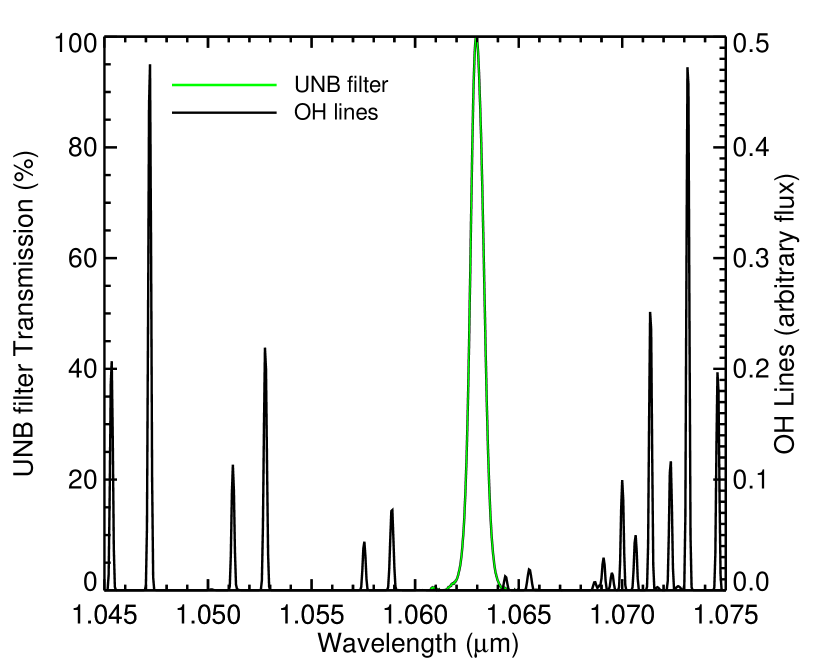
Figure 1.— Normalized narrowband filter transmission curve (green line) and night-sky OH emission lines (Rousselot et al., 2000) (black line) with arbitrary flux. Here we have shown the transmission curve (at the center of the field) of only narrowband filter to demonstrate the use of very narrow region between OH lines, to search for Ly$\alpha\;$ emitters at $z$=7.7. Two weak OH emission lines with $\lambda=1.05888$ and $1.05754\mu m$ (Rousselot et al., 2000) appear in the UNB images as concentric rings beyond 12’ radius, since the central wavelength of the UNB filter shifts to the blue for positions away from field center.

2.2. Data Reduction

We reduced UNB & J-band data using a combination of standard IRAF tasks, predominantly from the mscred (Valdes, 1998) and nfextern (Dickinson & Valdes, 2009) packages, along with custom IDL reduction procedures.

To remove OH rings from UNB data, we created a radial profile for each individual exposure, smoothed over a small radius interval $dr$, and subtracted this profile from the exposure. We then performed sky subtraction by median averaging two OH ring-subtracted frames that were taken immediately before and two frames after the science frame in consideration. We then performed cosmic ray rejection on sky-subtracted frames, using the algorithm of Rhoads (2000a). Prior to flat-fielding performed using dome-flats, we created a bad pixel mask for each science frame by combining the cosmic ray flagged pixels with a static bad pixel mask for the detector. We then replaced all bad pixels with zero (which is the background level in these sky-subtracted images) prior to any resampling of the frames. We adjusted the World Coordinate System of individual frames by matching the point sources to the 2MASS point source catalog using IRAF task $msccmatch$. We then combined the four chips (i.e four extensions) of each science exposure into a single simple image using the $mscimage$ task in IRAF, which interpolates the data onto a common pixel grid. Here we used $sinc17$ for the interpolation. Using mscstack in IRAF, we then stacked all of the narrowband exposures into a single, final narrowband stack. Pixels flagged as bad are omitted from the weighted averages in this step. The average FWHM of our final narrowband stack was 1.36$\arcsec$. In addition to this stacked image, we also generated individual night stacks, which were later used to identify glitches in Ly$\alpha\;$ candidate selection.

For broadband J-filter data reduction, we followed essentially the same procedure, modified by omission of the OH ring subtraction which is rendered unnecessary by the absence of noticeable OH rings in the much broader J bandpass.

We now assess the accuracy of sky subtraction method, the distribution of noise, and the uncertainty in the astrometric calibration of the UNB and J-band stacks. To evaluate the sky subtraction, and to understand the noise distribution we constructed sky background, and background noise maps using SExtractor (Bertin & Arnouts, 1996). The sky subtraction is sufficiently uniform throughout the image except in the corners i.e. beyond the OH lines affected regions. The noise, due to sky brightness, is also consistent with the expected Poisson noise distribution from sky photons.

To evaluate the uncertainty in the astrometric calibration, we compared the world coordinates of the sources in the UNB stack (obtained using SExtractor) and the corresponding object coordinates from the 2MASS catalog. We found that the uncertainty in the astrometric calibration is very small, and independent of the position in the UNB image. The rms of the matched coordinates of UNB and 2MASS is about 0.2 and 0.3 arcseconds corresponding to RA and DEC respectively.

We obtained reduced stacks of deep optical broadband data in B_w, R, and I filters, previously observed by the NOAO Deep Wide Field Survey (NDWFS).

At the end, we have one deep UNB stack, along with five single-night UNB stacks, four broadband stacks in J, B_w, R, and I filters, and four deep stacks in g^′, r^′, i^′ and z^′ (Finkelstein et al., 2009). All the stacks were then geometrically matched for ease of comparison.

2.3. Photometric Calibration

We performed photometric calibration of UNB & J-band $\rm(J_{NF})$ data by comparing unsaturated point sources, extracted using SExtractor, with 2MASS stars. From 2MASS catalog we selected only those stars that had J-band $\rm(J_{2M})$ magnitudes between 13.8 & 16.8 AB mag, and errors less than 0.1 magnitude. Since four quadrants of the UNB stack had slightly different zero-points, we scaled three quadrants, selected geometrically, to the fourth quadrant, which was closest to the mean zeropoint, by multiplying each quadrant with suitable scaling factors so as to make zero-point uniform throughout the image. We then obtained zero-points for UNB and $\rm J_{NF\;}$by minimizing the difference between UNB & $\rm J_{2M}\;$, and between $\rm J_{NF\;}$& $\rm J_{2M}\;$respectively. This left 0.09 rms mag between $\rm J_{2M}\;$& $\rm J_{NF\;}$magnitudes, and 0.07 rms mag between UNB & $\rm J_{2M}\;$magnitudes. The photometric calibration was based on about 30 & 80 2MASS stars for narrow-band and J-band respectively. So the accuracy of the photometric zero points is about $\pm 0.02$ mag in both J and UNB filters.

In addition to the error we have already estimated, there is some uncertainty arising due to different filter widths, and differing central wavelengths of the 2MASS and UNB filter. To estimate this uncertainty we constructed observed spectral energy distribution (SED) of stars that were common to both, the UNB image and $\rm g^{\prime},\;r^{\prime},\;i^{\prime},\;z^{\prime},\;J,\;H,\;\&\;K$ images. From each SED linearly interpolated flux at central wavelengths of the UNB filter and J-filter were measured. From these SEDs we found the median offset between the UNB and J band to be $<$ 0.1 mag. This residual color-term uncertainty in the photometric zero points is smaller than the photometric flux uncertainty in any of our Ly$\alpha\;$ candidates.

Before we proceed to calculate the limiting magnitudes, we estimate the sky brightness between the OH lines in the UNB image. To estimate this sky value, we construct the UNB stack in the same way as described in Section 2.2 but omitting the OH ring subtraction, and sky subtraction. In addition, we subtracted dark current counts from each raw frame. We estimated the average sky brightness in the UNB image by selecting 30 random regions avoiding astronomical objects and OH rings. This gives us the sky brightness, between the OH lines, of about 21.2 $\rm mag\;arcsec^{-2}$ equivalent to 162 photons $\rm s^{-1}\;m^{-2}\;arcsec^{-2}\;\mu m^{-1}$. This sky brightness is much fainter than the J-band sky brightness which is about 16.1 $\rm mag\;arcsec^{-2}$ equivalent to 17000 photons $\rm s^{-1}\;m^{-2}\;arcsec^{-2}\;\mu m^{-1}$ (Maihara et al., 1993) . However, more careful analysis are needed to estimate the interline sky brightness in the UNB images.

2.4. Limiting Magnitudes

To obtain limiting magnitudes of stacked images, we performed a series of artificial source simulations. In each, we introduced 400 artificial point sources in an 0.1 magnitude bin of flux in the final stacked image. The positions were chosen randomly, but constrained to avoid places close to bright stars and already existing sources. We then ran SExtractor, with the same parameters as were used for the real source detection (see Section 3), to calculate the fraction of recovered artificial sources. We ran 20 such simulations in each 0.1 magnitude bin from UNB = 21 to 24 mag. The 50$\%$ completeness level is UNB$=22.5$ mag, which corresponds to an emission line flux of $6\times 10^{-18}{\rm\,erg\,cm^{-2}\,s^{-1}}$. The very narrow bandpass results in a relatively bright continuum limit (compared to more conventional narrowband filters with $1\%$ to $1.5\%$ bandpass), but the conversion between narrowband magnitude and line flux is extremely favorable, so that our line flux limits are competitive with any narrowband search in the literature. The 50$\%$ completeness for other filters B_w, R, I, and $\rm J_{NF\;}$correspond to 26.3, 25.4, 25.0, and 23.5 mag respectively.

3. Ly$\alpha\;$ candidate selection

We identified sources in the stacked narrowband image using SExtractor. To measure their fluxes at other wavelengths, we first combined the broad-band optical images B_w, R, I into a single chi-squared image (Szalay et al., 1999) constructed using Swarp(Bertin et al., 2002). A chi-square image is constructed using the probability distribution of sky pixels in each of the images to be combined, and extracting the pixels that are dominated by object flux. We then used SExtractor in dual-image mode in order to measure object fluxes in both the broad J filter and the combined optical chi-squared image. In dual image mode, a detection image (UNB in this case) is used to identify the pixels associated with each object, while the fluxes are measured from a distinct photometry image.

To identify Ly$\alpha\;$ candidates in our survey, we used the combined optical image, UNB image, and J-band image. Each Ly$\alpha\;$ candidate had to satisfy all the following criteria:

• $5\sigma$ significant detection in the UNB filter,

• $3\sigma$ significant narrowband excess (compared to the J band image),

• flux density ratio $f_{\nu}(UNB)/f_{\nu}(J)>2$,

• non-detection in the combined chi-square optical image (with $<2\sigma$ significance),

• consistent with constant flux from night to night (see Section 3.1), and

• non-detection in individual optical images.

Criteria a-c ensure real emission line sources. Criterion d eliminates most low-redshift sources, e eliminates time variable sources and other glitches, and criterion f eliminates LBGs at $z\gtrsim 4$ which might show up more clearly in the R or I band than in the $\chi^{2}$ image We also used deeper optical images (Finkelstein et al., 2007) in the overlapping field between MMT/Megacam and NEWFIRM for criterion f.

The criteria follow the successful searches for Ly$\alpha\;$ galaxies at lower redshifts of z=4.5 and 5.7, which have $\approx 70-80\%$ spectroscopic success rate (Rhoads & Malhotra, 2001; Rhoads et al., 2003; Dawson et al., 2004, 2007; Wang et al., 2009).

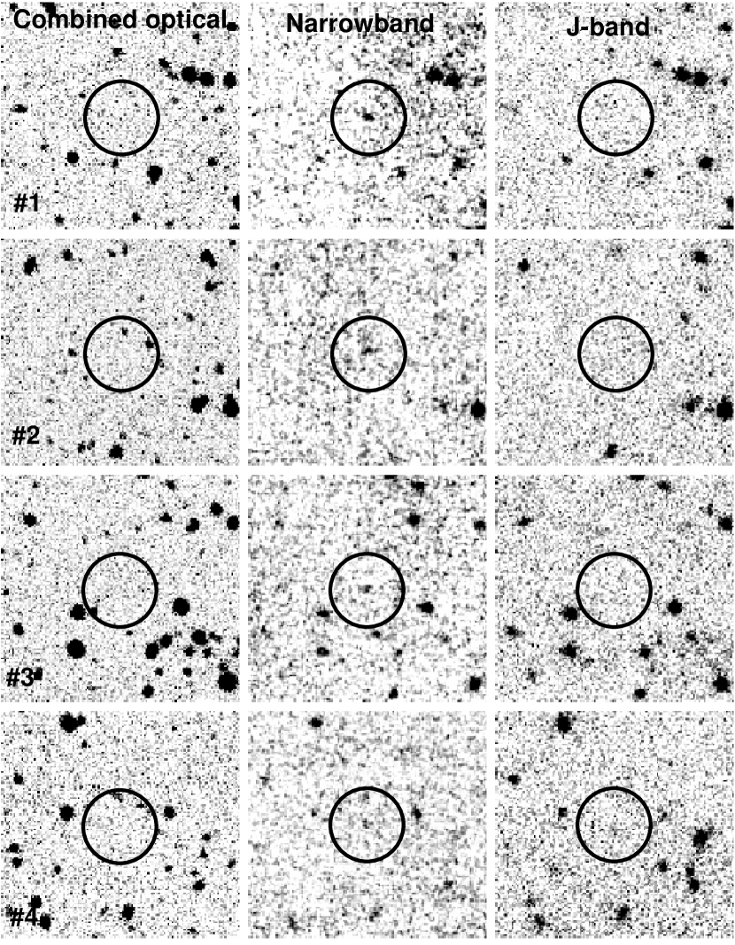
Figure 2.— Postage stamps (50^′′ wide) of all four Ly$\alpha\;$ candidates in combined (chi-square) optical image (left panel), UNB (middle), and J-band filter (right panel). The positions of Ly$\alpha\;$ candidates are marked with circles 16^′′ in diameter.

3.1. Constant flux test

In our constant flux test (criterion e above), we looked at the variation of flux of each Ly$\alpha\;$candidate over five nights. We reject any source having individual night stack fluxes close to zero or showing flux variations above a certain chi-square value. To do this, we generated light-curves of each candidate using individual night stacks of UNB, and then determined the $\chi^{2}$ of the data with respect to the best-fitting constant flux. Since we had five nights of data, we selected only those candidate that had a chi-square $<$5. This is in addition to requiring $s/n>5$, which guards against peaks in the sky noise entering the candidate list.

We also eliminated all the sources that were very close to the chip boundaries. Combining these criteria with the set of criteria from Section 3, we had six Ly$\alpha\;$ emitter candidates. To increase the reliability of these candidates, we finally selected four candidates after independent visual inspection by four of the authors. Figure 2 shows postage stamps of all four Ly$\alpha\;$ candidates. The candidates are clearly visible in the UNB images (middle panel), while undetected in the combined optical (left panel), and J band images (right panel). We provide the coordinates of our Ly$\alpha\;$ candidates in Table 1.

Table 1Coordinates of our Ly$\alpha\;$ candidates.

	RA(J2000)	DEC (J2000)
LAE 1	02:04:45.9	-04:53:00.8
LAE 2	02:04:41.3	-05:00:11.5
LAE 3	02:04:53.2	-04:46:43.8
LAE 4	02:05:58.0	-05:05:48.4

4. Contamination of the sample

While we have carefully selected Ly$\alpha\;$ candidates based on photometric and geometric criteria, it is possible that our Ly$\alpha\;$ candidates can be contaminated by sources that include transient objects such as supernova, cool stars (L & T dwarfs), foreground emission line sources, and electronic noise in the detector. We now discuss the possible contribution of sources that can contaminate our Ly$\alpha\;$ candidate sample.

4.1. Foreground emission line objects

Our Ly$\alpha\;$ candidate selection can include foreground emission line sources including [O ii] emitters ($\lambda=3727\rm\AA$) at $z$=1.85, [O iii] ($\lambda=5007\rm\AA$) emitters at $z$=1.12, and H$\rm\alpha$($\lambda=6563\rm\AA$) emitters at $z$=0.62, if they have strong emission line flux but faint continuum emission. We now estimate the number of foreground emitters that can pass our Ly$\alpha\;$ candidate selection criteria.

In our UNB stack, the 50% completeness limit corresponds to a flux of $6\times 10^{-18}\rm erg\;s^{-1}\;cm^{-2}$. Therefore the minimum luminosities required by the foreground emission line sources to be detected in our survey are $1.5\times 10^{41}\rm erg\;s^{-1}$, $4\times 10^{40}\rm erg\;s^{-1}$, and $1\times 10^{40}\rm erg\;s^{-1}$ for [O ii], [O iii], and H$\rm\alpha$ emitters respectively.

Given the depth of our combined optical image, we can calculate the minimum observer frame equivalent width (EW_min) that would be required for an emission line object to be a Ly$\alpha\;$ emitter candidate. We calculated the observer frame EW using the following relation (Rhoads & Malhotra, 2001):

$$\rm EW_{min}\approx\left[\frac{f_{nb}}{f_{bb}}-1\right]\;\Delta\lambda_{nb}=\left[\frac{5\sigma_{nb}}{2\sigma_{bb}}-1\right]\;\Delta\lambda_{nb}$$ (1)

where $\rm f_{nb}\;and\;f_{bb}$ are the fluxes in UNB and combined optical image respectively, $\rm\Delta\lambda_{nb}$ is the UNB filter width, and $\rm\sigma_{nb}\;and\;\sigma_{bb}$ are the uncertainties in flux measurements in UNB and combined optical image respectively. (The implicit approximation that the continuum contributes negligibly to the narrowband flux, is well justified for our 9Å bandpass.) With $\rm 5\sigma_{nb}=7.8\times 10^{-29}erg\;cm^{-2}s^{-1}Hz^{-1}\;and\;2\sigma_{bb}=1.5\times 10^{-30}erg\;cm^{-2}s^{-1}Hz^{-1}$, we found that the foreground emission line sources would require $\rm EW_{min}\gtrsim 460\AA$ to contaminate our Ly$\alpha\;$candidate sample.

Foreground [O ii]and [O iii] emitters: Unfortunately, the equivalent width distribution of [O ii] emitters has not been directly measured at $z$=1.85. However, several authors (Teplitz et al., 2003; Kakazu et al., 2007; Straughn et al., 2009) have studied [O ii] emitters at $z<$1.5. Here we use [O ii] EW distribution, obtained by Straughn et al. (2009) at $\langle z\rangle\approx$1 in GOODS-south field, with the assumption that there is no significant evolution of the [O ii] LF from $z$=1 to $z$=1.85. In our Ly$\alpha\;$ candidate selection, emission line sources with $I_{AB}$ fainter than 25.9 magnitude, and with $\rm EW_{obs}>460\AA$ can contaminate our sample. We determined which sources from Straughn et al. (2009) would have passed these criteria if redshifted to $z=1.85$, and scaled the result by the ratio of volumes between the two surveys. We find that less than one (0.1) [OII] emitter is expected to contaminate our Ly$\alpha\;$ candidate sample. To be conservative, even if we relax the above magnitude cut by 0.5 mag to account for any color correction, and lower the $\rm EW_{obs}>200\AA$, we find that less than 0.3 [O ii] emitters should be expected to contaminate our sample.

We apply a similar methodology to estimate the contamination from foreground [O iii] emitters (Kakazu et al., 2007; Hu et al., 2009; Straughn et al., 2009, 2010) at $\langle z\rangle\approx 1.1$ in our NEWFIRM data using the [O iii] emission line sources at $\langle z\rangle=$0.5 in Straughn et al. (2009). We found that less than two (1.7) [O iii] emitters can be misidentified as Ly$\alpha\;$ emitters in our survey. In addition to the above estimate, we used a recent sample of emission line galaxies obtained from HST WFC3 early release science data (Straughn et al., 2010). This sample of [O iii] emitters is closer in redshift, with median $z=1.1$, to our foreground [O iii] interloper redshift of $z=1.12$, thus minimizing the error in our [O iii] estimate due to possible evolution in the LF of [O iii] emitters. Using this recent sample, we found that about one [O iii] emitter is expected to contaminate our Ly$\alpha\;$ candidate sample.

Foreground H${\alpha}$ emitters: As mentioned earlier, H${\alpha}$ emitters at $z$=0.62 can contaminate our Ly$\alpha\;$candidate sample. Several authors (Tresse et al., 2002; Straughn et al., 2009) have studied H${\alpha}$ emitters at similar redshift. Tresse et al. (2002) (see their Figure 6) have plotted the $\rm H{\alpha}\;$luminosity vs the continuum B-band magnitude of $\rm H{\alpha}\;$emitters. To pass our selection criteria, an $\rm H{\alpha}\;$emitter would require a luminosity greater than $1\times 10^{40}\rm erg\;s^{-1}$, and flux density $f_{B_{w}}<7.5\times 10^{-20}\rm erg\;cm^{-2}s^{-1}Hz^{-1}$ which corresponds to $\rm M_{AB}=-15.97$ mag. Any source brighter than $\rm M_{AB}$=-15.97 mag would be detected in the $B_{w}$ image, and hence rejected from Ly$\alpha\;$candidate list. From figure 6 (Tresse et al., 2002), we expect to find no sources that can pass this selection criteria. In addition, we used H${\alpha}$ emitters at $\langle z\rangle$=0.27 (Straughn et al., 2009), and found that less than one (0.4) H${\alpha}$ emitters are expected to contaminate our Ly$\alpha\;$ candidate sample.

4.2. Other Contaminants

Transient objects : We rule out the possibility of contamination of our Ly$\alpha\;$ candidates by transient objects such as supernovae, because these objects would appear in both UNB and J band stacks. Both UNB and J data were obtained on each clear night of the run.

L and T Dwarfs : Following Hibon et al. (2009) we determined the expected number of L/T dwarfs in our survey. From the spectral type vs. absolute magnitude relations given by figure 9 in Tinney et al. (2003), we infer that we could detect L dwarfs at a distance of 400 to 1300 pc and T dwarfs at a distance of 150 to 600 pc, from the coolest to the warmest spectral types.

Our field is located at a high galactic latitude, so that we would be able to detect L/T dwarfs well beyond the Galactic disk scale height. However, only a Galactic disk scale height of 350 pc is applicable to the population of L/T dwarfs (Ryan et al., 2005). We derive then a sampled volume of $\sim$ 750 pc³. Considering a volume density of L/T dwarfs of a few 10^-3 pc^-3, we expect no more than one L/T dwarf in our field.

While we expect about one L/T dwarf in our survey, we further investigate if any of the observed L/T dwarf pass our selection criteria. To do this we selected about 160 observed spectra of L/T dwarf (Golimowski et al., 2004; Knapp et al., 2004; Chiu et al., 2006), and calculated the flux transmitted through the UNB and J-band filter. We found that none of the L/T dwarf has sufficient narrowband excess to pass our selection criteria. Therefore it is unlikely that our Ly$\alpha\;$ candidate sample is contaminated by L/T dwarf.

Noise Spikes: Noise in the detector can cause random flux increase in the UNB filter. To avoid contamination from such noise spikes, we constructed light curves of each candidate using individual night stacks i.e. we selected candidates only if their flux was constant over all nights. This method of candidate selection based on the constant flux in the individual night stacks also eliminates the possible contamination from persistence.

Contribution from false detection: Finally, we performed a false detection test to estimate the number of false detection that can pass our Ly$\alpha\;$ selection criteria. To do this we multiplied the UNB stack by -1 and repeated the exact same procedure as the real Ly$\alpha\;$ candidate selection (see section 3). We did not get any false detection passing our selection criteria.

5. Monte-Carlo Simulations

Based on the above estimates less than two [O iii] emitters are expected to be misidentified as Ly$\alpha\;$ emitters in our survey. To estimate the number of sources that should be detected in our survey for a given Ly$\alpha\;$ LF, we performed detailed Monte-Carlo simulations. This is needed, since the width of the filter is comparable to or slightly smaller than the expected line width in these galaxies, so many of the sources will not be detected at their real line fluxes. In these simulations, we used the $z=6.6$ Ly$\alpha\;$ LF derived by Kashikawa et al. (2006).

First, we generated one million random galaxies distributed according to the observed Ly$\alpha\;$ LF at $z$=6.6 (Kashikawa et al., 2006). Each of these galaxies was assigned a Ly$\alpha\;$ luminosity in the range $\rm 1\times 10^{42}<Ly\alpha<1.5\times 10^{43}erg\;s^{-1}$. Here we assumed that the Ly$\alpha\;$ LF does not evolve from $z$=6.6 to $z$=7.7. Each galaxy was then assigned a random redshift $z_{L}<z<z_{H}$ where $z_{L}$ and $z_{H}$ correspond to the minimum and maximum wavelengths where the transmission of the UNB filter drops to zero.

Next, to each galaxy we assigned a flux $\rm F=L_{Ly\alpha}/4\pi d_{L}^{2}$ where $\rm d_{L}$ is the luminosity distance. We distribute this flux in wavelength using an asymmetric Ly$\alpha\;$  line profile drawn from the $z=5.7$ spectra of Rhoads et al. (2003). The flux transmitted through the UNB filter was then determined as $f_{trans}=\int f_{\lambda}T_{\lambda}d\lambda$ (where $T_{\lambda}$ is the filter transmission and $f_{\lambda}$ the flux density of the emission line). This accounts for the loss of the Ly$\alpha\;$ flux that results from a filter whose width is comparable to the line width (and not much greater as would be the case for a 1% filter). We then created a histogram of magnitudes after converting the convolved flux to magnitudes calculated using the following relation:

$$\rm mag_{AB}=-2.5\;Log_{10}\left(\it\frac{f_{trans}}{f_{0}}\right),$$ (2)

and

$$f_{0}=\frac{\rm 3.6\;kJy\times c}{(1.06\mu)^{2}}\times\int T_{\lambda}\;d\lambda\;\;\;\rm erg\;s^{-1}cm^{-2},$$ (3)

with $c$ the speed of light.

Lastly, to include the instrumental effects, we multiplied the number of galaxies in each magnitude bin by the corresponding recovery fraction obtained from our artificial source simulations in our UNB image(see section 2.4). We then converted each magnitude bin to a Ly$\alpha\;$ luminosity bin, and counted the number of detected galaxies in each luminosity bin.

We repeated this simulation ten times, and taking an average, we found that about one Ly$\alpha\;$ emitter should be expected in our survey. It should be noted that we assumed a non-evolving Ly$\alpha\;$ LF from $z$=6.6 to $z$=7.7, and that every Ly$\alpha\;$ emitter has the same asymmetric Ly$\alpha\;$ line profile. While we expect about one Ly$\alpha\;$ emitter in our survey there are large uncertainties mainly due to the Poisson noise, and field to field variation or cosmic variance. Tilvi et al. (2009) have estimated field to field variation of Ly$\alpha\;$ emitters to be $\gtrsim 30\%$ for a volume and flux limited Ly$\alpha\;$ survey with a survey volume $\rm\sim 2\times 10^{5}\;Mpc^{3}$. We expect a larger field to field variation for smaller survey volumes. We also estimated the cosmic variance expected in our survey using the cosmic variance calculator (Trenti & Stiavelli, 2008). For our survey we should expect a cosmic variance of about $58\%$ assuming an intrinsic number of Ly$\alpha\;$ sources at $z=7.7$ in agreement with a non-evolving Ly$\alpha\;$ LF from $z=6.6$ (Kashikawa et al., 2006) to $z=7.7$. On the other hand our candidate counts are quite consistent with the luminosity function at z=5.7 (Ouchi et al., 2009).

Figure 3.— Cumulative Ly$\alpha\;$  luminosity function of our $z$=7.7 candidates (filled circles). The filled points show the LF that will result if all four Ly$\alpha\;$ galaxy candidates are confirmed. The upper error bars are Poisson errors based on our sample size, while the down-arrows below each data point indicate the possibility of a lower LF if some candidates are extreme emission line galaxies at lower redshift. The open circles represent the LF from Hibon et al. (2009) while the dashed line and dotted line show Ly$\alpha\;$ LFs at $z$=5.7 (Ouchi et al., 2008) and $z$=6.5 (Kashikawa et al., 2006) respectively. The open square is the LF at $z$=6.96 (Iye et al., 2006).

6. Ly$\alpha\;$ luminosity function at $z$=7.7

Using a large sample of Ly$\alpha\;$candidates, Ouchi et al. (2008) found no significant evolution of Ly$\alpha\;$ LF between $z$=3.1 and $z$=5.7. The evolution of the Ly$\alpha\;$ LF between $z=$5.7 and $z=6.5$ is not conclusive. For example, Malhotra & Rhoads (2004) found no significant evolution of Ly$\alpha\;$ LF between $z$=5.7 and $z=6.5$, while Kashikawa et al. (2006) suggest an evolution of bright end of the LF in this redshift range. On the theoretical front, several models (Thommes & Meisenheimer, 2005; Furlanetto et al., 2005; Le Delliou et al., 2006; Dijkstra et al., 2007; Kobayashi et al., 2007; McQuinn et al., 2007; Dayal et al., 2008; Nagamine et al., 2008; Samui et al., 2009; Tilvi et al., 2009) have been developed to predict redshift evolution of the Ly$\alpha\;$ LF. While several models (e.g. Samui et al., 2009; Tilvi et al., 2009) predict no significant evolution of Ly$\alpha\;$ LF at $z\lesssim 7$, the predictions differ greatly among different models. These differences among the models can be attributed to differing input assumptions, which in turn stem from our imperfect understanding of the physical nature of Ly$\alpha\;$ galaxies, and from the small samples currently available at high redshift.

Table 2 Ly$\alpha\;$ searches at $z>$7.

$z$	Survey	Detection limits	No. of LAE	Ref.
	volume (Mpc3)	erg s-1	candidates
7.7	$1.4\times 10^{4}$	$6\times 10^{-18}$	4	This study
7.7	$6.3\times 10^{4}$	$8.3\times 10^{-18}$	7	Hibon et al 2009
8-10	$35$	$2\times 10^{-17}$	6	Stark et al 2007
8.8	3 arcmin2	$\sim 10^{-18}$	0	Parkes et al 1994
8.8	$991$	$2\times 10^{-17}$	0	Willis et al 2005
8.8	$6.3\times 10^{4}$	$1.3\times 10^{-17}$	0	Cuby et al 2007
8.96	$1.12\times 10^{6}$	$6\times 10^{-17}$	0	Sobral et al 2009
$\sim 9$	$\sim 450$	$3.7\times 10^{-18}$	0	Willis et al 2008

At $z>$ 6.5, there are only a few searches for Ly$\alpha\;$ emitters. Iye et al. (2006) found one spectroscopically confirmed LAE at $z$=6.96, and currently there are no spectroscopically confirmed LAEs at $z>$ 7. However, there are few photometric searches (Parkes et al., 1994; Willis & Courbin, 2005; Cuby et al., 2007; Hibon et al., 2009) for Ly$\alpha\;$ galaxies, and constraints on Ly$\alpha\;$ LF at $z>$ 7. Table 2 shows details of different Ly$\alpha\;$ searches at $z>$7.

After careful selection of Ly$\alpha\;$ candidates and eliminating possible sources of contamination, we have found four Ly$\alpha\;$ emitter candidates in a survey area of $28\times 28$ arcmin², with a limiting flux of $\rm 6\times 10^{-18}erg\;s^{-1}\;cm^{-2}$ . The fluxes of these four candidates are 1.1, 0.91, 0.84 and 0.72 in units of $\rm 10^{-17}\;erg\;s^{-1}\;cm^{-2}$. Fig. 3 shows the resulting cumulative Ly$\alpha\;$ luminosity function. Solid filled circles show the Ly$\alpha\;$ LF derived from our candidates, while open circles represent Ly$\alpha\;$LF from Hibon et al. (2009). Arrows indicate that this is the upper limit on the Ly$\alpha\;$ LF, and upper error bars are the Poisson errors. The dotted and dashed lines show Ly$\alpha\;$ LFs from Ouchi et al. (2008) and Kashikawa et al. (2006) respectively. The open square is the Ly$\alpha\;$ LF at $z$=6.96 (Iye et al., 2006).

If all of our Ly$\alpha\;$candidates are $z$=7.7 galaxies, the LF derived from our sample shows moderate evolution compared to LF at $z$=6.5 (Kashikawa et al., 2006). On the other hand, conservatively if only one of the candidates is a $z=7.7$ galaxy, then the Ly$\alpha\;$ LF does not show any evolution compared to the $z=6.6$ Ly$\alpha\;$ LF. Hibon et al. (2009) conclude that the observed Ly$\alpha\;$ LF at $z=7.7$ does not evolve significantly compared to Ly$\alpha\;$ LF at $z$=6.5 (Kashikawa et al., 2006), if they consider that all of their candidates are real. Finally, while our Ly$\alpha\;$ LF lies above the LF obtained by Hibon et al. (2009), the counts are consistent with the number of star-forming galaxies in the HUDF with inferred Ly$\alpha\;$ line fluxes $\rm>6\times 10^{-18}erg\;s^{-1}\;cm^{-2}$ (Finkelstein et al., 2009b), and also consistent with the Ly$\alpha\;$ LF at $z$=5.7 (Ouchi et al., 2008).

As described in Section 5, all surveys for Ly$\alpha\;$ emitters at $z>6$ suffer from cosmic variance. We do expect to see field-to-field variation in number counts even at the same redshift. Therefore it is important to get statistics from more than one field for each redshift. The field-to-field variation is expected to be stronger for brighter sources. Therefore the higher redshift surveys, which are more sensitivity limited, are hit the hardest.

7. Ly$\alpha\;$ Equivalent Width

Several studies have found numerous Ly$\alpha\;$emitters having large rest-frame equivalent widths, $\rm EW_{rest}>240\AA$ (Malhotra & Rhoads, 2002; Shimasaku et al., 2006; Dawson et al., 2007; Gronwall et al., 2007; Ouchi et al., 2008). These exceed theoretical predictions for normal star forming galaxies.

Since the J-band filter does not include the Ly$\alpha\;$ line, we have used the following relation to calculate the rest-frame Ly$\alpha\;$ EWs for our four Ly$\alpha\;$ candidates:

$$\rm EW_{rest}=\frac{f_{NB}}{f_{\lambda,BB}}\times\frac{1}{(1+z)}~{}~{}.$$ (4)

Here $\rm f_{{NB}}$ and $\rm f_{\lambda,{BB}}$ are the UNB line flux ($\rm erg\;s^{-1}cm^{2}$), and J-band flux (erg s^-1 cm² Å^-1) respectively. Since none of the four candidates are detected in J-band, we used J-band limiting magnitude to calculate a lower limit on the Ly$\alpha\;$ EWs. We note that the Ly$\alpha\;$EW will depend on the exact redshift, shape, and precise position of the Ly$\alpha\;$line in the UNB filter. However, for simplicity and because we only put lower limits on EWs, we assume that the UNB filter encloses all the Ly$\alpha\;$line flux in calculating EWs.

For our Ly$\alpha\;$ candidates, with line flux estimates from $7$ to $11\times 10^{-18}{\rm\,erg\,cm^{-2}\,s^{-1}}$, and our broad band limit $J_{NF}\geq 23.5$ mag, we find Ly$\alpha\;$  $\rm EW_{rest}\gtrsim 3\AA$.

This EW limit is considerably smaller than the $\rm EW_{rest}>9\AA$ obtained by Hibon et al. (2009) for their Ly$\alpha\;$  candidates at $z$=7.7. This difference arises due to the smaller bandwidth of our UNB filter, and our somewhat shallower J band imaging. Deep J-band observations will help in getting either measurements or stricter lower limits on the line EWs, but will also be observationally challenging.

8. Summary and Conclusions

We have performed a deep, wide field search for $z=$7.7 Ly$\alpha\;$ emitters on the NEWFIRM camera at the KPNO 4m Mayall telescope. We used an ultra-narrowband filter with width 9$\rm\AA$ and central wavelength of 1.063$\mu m$, yielding high sensitivity to narrow emission lines.

After careful selection of candidates by eliminating possible sources of contamination, we detected four candidate Ly$\alpha\;$ emitters with line flux $\rm>6\times 10^{-18}erg\;s^{-1}\;cm^{-2}$ in a comoving volume of $\rm 1.4\times 10^{4}\;Mpc^{3}$. While we have carefully selected these four Ly$\alpha\;$ candidates, we note that the number of Ly$\alpha\;$  candidates is more than the expected number obtained by using the z=6.6 luminosity function of Kashikawa et al. 2006, though quite consistent with the z=5.7 luminosity function of Ouchi et al. (2008). Hence, our results would allow for a modest increase in the Ly$\alpha\;$ LF from $z=6.5$ to $z\approx 8$. Spectroscopic confirmation of more than two candidates would show that such an increase is in fact required. However, more surveys are needed to account for the uncertainty due to cosmic variance.

In order to use the Ly$\alpha\;$ luminosity functions as a test of reionization, we need to be able to detect variations in $L^{\star}$, the characteristic luminosity, of factors of three or four. This will require larger samples, spectroscopic confirmations, and a measure of field-to-field variation.

It is therefore premature to draw any conclusions about reionization from the current sample. It is, however, encouraging that we are able to reach the sensitivity and volume required to detect multiple candidates robustly.

References

- Ajiki et al. (2004) Ajiki, M., et al. 2004, PASJ, 56, 597
- Autry et al. (2003) Autry, R. G., et al. 2003, Proc. SPIE, 4841, 525
- Bertin & Arnouts (1996) Bertin, E., & Arnouts, S. 1996, A&AS, 117, 393
- Bertin et al. (2002) Bertin, E., Mellier, Y., Radovich, M., Missonnier, G., Didelon, P., & Morin, B. 2002, Astronomical Data Analysis Software and Systems XI, 281, 228
- Chiu et al. (2006) Chiu, K., Fan, X., Leggett, S. K., Golimowski, D. A., Zheng, W., Geballe, T. R., Schneider, D. P., & Brinkmann, J. 2006, AJ, 131, 2722
- Cowie & Hu (1998) Cowie, L. L., & Hu, E. M. 1998, AJ, 115, 1319
- Cuby et al. (2007) Cuby, J.-G., Hibon, P., Lidman, C., Le Fèvre, O., Gilmozzi, R., Moorwood, A., & van der Werf, P. 2007, A&A, 461, 911
- Dawson et al. (2004) Dawson, S., et al. 2004, ApJ, 617, 707
- Dawson et al. (2007) Dawson, S., Rhoads, J. E., Malhotra, S., Stern, D., Wang, J., Dey, A., Spinrad, H., & Jannuzi, B. T. 2007, ApJ, 671, 1227
- Dayal et al. (2008) Dayal, P., Ferrara, A., & Gallerani, S. 2008, MNRAS, 389, 1683
- Dickinson & Valdes (2009) Dickinson, M. & Valdes, F. A Guide to NEWFIRM Data Reduction with IRAF, NOAO SDM PL017, 2009
- Dijkstra et al. (2007) Dijkstra, M., Wyithe, J. S. B., & Haiman, Z. 2007, MNRAS, 379, 253
- Furlanetto et al. (2005) Furlanetto, S. R., Schaye, J., Springel, V., & Hernquist, L. 2005, ApJ, 622, 7
- Furlanetto et al. (2006) Furlanetto, S. R., Zaldarriaga, M., & Hernquist, L. 2006, MNRAS, 365, 1012
- Finkelstein et al. (2007) Finkelstein, S. L., Rhoads, J. E., Malhotra, S., Pirzkal, N., & Wang, J. 2007, ApJ, 660, 1023
- Finkelstein et al. (2009) Finkelstein, S. L., Rhoads, J. E., Malhotra, S., & Grogin, N. 2009, ApJ, 691, 465
- Finkelstein et al. (2009b) Finkelstein, S. L., Papovich, C., Giavalisco, M., Reddy, N. A., Ferguson, H. C., Koekemoer, A. M., & Dickinson, M. 2009, arXiv:0912.1338
- Fynbo et al. (2001) Fynbo, J. U., Möller, P., & Thomsen, B. 2001, A&A, 374, 443
- Gawiser et al. (2006) Gawiser, E., et al. 2006, ApJ, 642, L13
- Golimowski et al. (2004) Golimowski, D. A., et al. 2004, AJ, 127, 3516
- Gronwall et al. (2007) Gronwall, C., et al. 2007, ApJ, 667, 79
- Hibon et al. (2009) Hibon, P., et al. 2009, arXiv:0907.3354
- Horton et al. (2004) Horton, A., Parry, I., Bland-Hawthorn, J., Cianci, S., King, D., McMahon, R., & Medlen, S. 2004, Proc. SPIE, 5492, 1022
- Hu et al. (1999) Hu, E. M., McMahon, R. G., & Cowie, L. L. 1999, ApJ, 522, L9
- Hu et al. (2002) Hu, E. M., Cowie, L. L., McMahon, R. G., Capak, P., Iwamuro, F., Kneib, J.-P., Maihara, T., & Motohara, K. 2002, ApJ, 568, L75
- Hu et al. (2004) Hu, E. M., Cowie, L. L., Capak, P., McMahon, R. G., Hayashino, T., & Komiyama, Y. 2004, AJ, 127, 563
- Hu et al. (2009) Hu, E. M., Cowie, L. L., Kakazu, Y., & Barger, A. J. 2009, ApJ, 698, 2014
- Iye et al. (2006) Iye, M., et al. 2006, Nature, 443, 186
- Jannuzi & Dey (1999) Jannuzi, B. T., & Dey, A. 1999, Photometric Redshifts and the Detection of High Redshift Galaxies, 191, 111
- Kakazu et al. (2007) Kakazu, Y., Cowie, L. L., & Hu, E. M. 2007, ApJ, 668, 853
- Kashikawa et al. (2006) Kashikawa, N., et al. 2006, ApJ, 648, 7
- Knapp et al. (2004) Knapp, G. R., et al. 2004, AJ, 127, 3553
- Kobayashi et al. (2007) Kobayashi, M. A. R., Totani, T., & Nagashima, M. 2007, ApJ, 670, 919
- Kodaira et al. (2003) Kodaira, K., et al. 2003, PASJ, 55, L17
- Komatsu et al. (2010) Komatsu, E., et al. 2010, arXiv:1001.4538
- Kudritzki et al. (2000) Kudritzki, R.-P., et al. 2000, ApJ, 536, 19
- Le Delliou et al. (2006) Le Delliou, M., Lacey, C. G., Baugh, C. M., & Morris, S. L. 2006, MNRAS, 365, 712
- Maihara et al. (1993) Maihara, T., Iwamuro, F., Yamashita, T., Hall, D. N. B., Cowie, L. L., Tokunaga, A. T., & Pickles, A. 1993, PASP, 105, 940
- Malhotra & Rhoads (2002) Malhotra, S., & Rhoads, J. E. 2002, ApJ, 565, L71
- Malhotra & Rhoads (2004) Malhotra, S., & Rhoads, J. E. 2004, ApJ, 617, L5
- Malhotra & Rhoads (2006) Malhotra, S., & Rhoads, J. E. 2006, ApJ, 647, L95
- McQuinn et al. (2007) McQuinn, M., Hernquist, L., Zaldarriaga, M., & Dutta, S. 2007, MNRAS, 381, 75
- Nagamine et al. (2008) Nagamine, K., Ouchi, M., Springel, V., & Hernquist, L. 2008, arXiv:0802.0228
- Nilsson et al. (2007) Nilsson, K. K., et al. 2007, A&A, 471, 71
- Ota et al. (2008) Ota, K., et al. 2008, ApJ, 677, 12
- Ouchi et al. (2001) Ouchi, M., et al. 2001, ApJ, 558, L83
- Ouchi et al. (2003) Ouchi, M., et al. 2003, ApJ, 582, 60
- Ouchi et al. (2008) Ouchi, M., et al. 2008, ApJS, 176, 301
- Ouchi et al. (2009) Ouchi, M., et al. 2009, ApJ, 696, 1164
- Papovich et al. (2001) Papovich, C., Dickinson, M., & Ferguson, H. C. 2001, ApJ, 559, 620
- Parkes et al. (1994) Parkes, I. M., Collins, C. A., & Joseph, R. D. 1994, MNRAS, 266, 983
- Pentericci et al. (2000) Pentericci, L., et al. 2000, A&A, 361, L25
- Pentericci et al. (2009) Pentericci, L., Grazian, A., Fontana, A., Castellano, M., Giallongo, E., Salimbeni, S., & Santini, P. 2009, A&A, 494, 553
- Pirzkal et al. (2007) Pirzkal, N., Malhotra, S., Rhoads, J. E., & Xu, C. 2007, ApJ, 667, 49
- Ryan et al. (2005) Ryan, R. E., Jr., Hathi, N. P., Cohen, S. H., & Windhorst, R. A. 2005, ApJ, 631, L159
- Rhoads (2000a) Rhoads, J. E. 2000, PASP, 112, 703
- Rhoads et al. (2000b) Rhoads, J. E., Malhotra, S., Dey, A., Stern, D., Spinrad, H., & Jannuzi, B. T. 2000, ApJ, 545, L85
- Rhoads & Malhotra (2001) Rhoads, J. E., & Malhotra, S. 2001, ApJ, 563, L5
- Rhoads et al. (2003) Rhoads, J. E., et al. 2003, AJ, 125, 1006
- Rhoads et al. (2004) Rhoads, J. E., et al. 2004, ApJ, 611, 59
- Rousselot et al. (2000) Rousselot, P., Lidman, C., Cuby, J.-G., Moreels, G., & Monnet, G. 2000, A&A, 354, 1134
- Samui et al. (2009) Samui, S., Srianand, R., & Subramanian, K. 2009, MNRAS, 398, 2061
- Shapley et al. (2001) Shapley, A. E., Steidel, C. C., Adelberger, K. L., Dickinson, M., Giavalisco, M., & Pettini, M. 2001, ApJ, 562, 95
- Shimasaku et al. (2006) Shimasaku, K., et al. 2006, PASJ, 58, 313
- Sobral et al (2009) Sobral, D., et al 2009, MNRAS, 398, L68
- Stark et al. (2007) Stark, D. P., Ellis, R. S., Richard, J., Kneib, J.-P., Smith, G. P., & Santos, M. R. 2007, ApJ, 663, 10
- Stark et al. (2009) Stark, D. P., Ellis, R. S., Bunker, A., Bundy, K., Targett, T., Benson, A., & Lacy, M. 2009, ApJ, 697, 1493
- Steidel et al. (1996) Steidel, C. C., Giavalisco, M., Pettini, M., Dickinson, M., & Adelberger, K. L. 1996, ApJ, 462, L17
- Stern et al. (2005) Stern, D., Yost, S. A., Eckart, M. E., Harrison, F. A., Helfand, D. J., Djorgovski, S. G., Malhotra, S., & Rhoads, J. E. 2005, ApJ, 619, 12
- Stiavelli et al. (2001) Stiavelli, M., Scarlata, C., Panagia, N., Treu, T., Bertin, G., & Bertola, F. 2001, ApJ, 561, L37
- Straughn et al. (2009) Straughn, A. N., et al. 2009, AJ, 138, 1022
- Straughn et al. (2010) Straughn, A. N., et al. 2010, arXiv:1005.3071
- Szalay et al. (1999) Szalay, A. S., Connolly, A. J., & Szokoly, G. P. 1999, AJ, 117, 68
- Taniguchi et al. (2005) Taniguchi, Y., et al. 2005, PASJ, 57, 165
- Teplitz et al. (2003) Teplitz, H. I., Collins, N. R., Gardner, J. P., Hill, R. S., & Rhodes, J. 2003, ApJ, 589, 704
- Thommes & Meisenheimer (2005) Thommes, E., & Meisenheimer, K. 2005, A&A, 430, 877
- Tilvi et al. (2009) Tilvi, V., Malhotra, S., Rhoads, J. E., Scannapieco, E., Thacker, R. J., Iliev, I. T., & Mellema, G. 2009, ApJ, 704, 724
- Tinney et al. (2003) Tinney, C. G., Burgasser, A. J., & Kirkpatrick, J. D. 2003, AJ, 126, 975
- Tokunaga et al. (2002) Tokunaga, A. T., Simons, D. A., & Vacca, W. D. 2002, PASP, 114, 180
- Trenti & Stiavelli (2008) Trenti, M., & Stiavelli, M. 2008, ApJ, 676, 767
- Tresse et al. (2002) Tresse, L., Maddox, S. J., Le Fèvre, O., & Cuby, J.-G. 2002, MNRAS, 337, 369
- Valdes (1998) Valdes, F. G. 1998, Astronomical Data Analysis Software and Systems VII, 145, 53
- Venemans et al. (2004) Venemans, B. P., et al. 2004, A&A, 424, L17
- Wang et al. (2004) Wang, J. X., et al. 2004, ApJ, 608, L21
- Wang et al. (2007) Wang, J. X., Zheng, Z. Y., Malhotra, S., Finkelstein, S. L., Rhoads, J. E., Norman, C. A., & Heckman, T. M. 2007, ApJ, 669, 765
- Wang et al. (2009) Wang, J.-X., Malhotra, S., Rhoads, J. E., Zhang, H.-T., & Finkelstein, S. L. 2009, ApJ, 706, 762
- Willis & Courbin (2005) Willis, J. P., & Courbin, F. 2005, MNRAS, 357, 1348
- Willis et al. (2008) Willis, J. P., Courbin, F., Kneib, J.-P., & Minniti, D. 2008, MNRAS, 384, 1039