Phase transitions in a three dimensional $U(1)\times U(1)$ lattice London superconductor

Abstract

We consider a three-dimensional lattice $U(1)\times U(1)$ superconductor in the London limit, with two individually conserved condensates. The problem, generically, has two types of intercomponent interactions of different characters. First, the condensates are interacting via a minimal coupling to the same fluctuating gauge field. A second type of coupling is the direct dissipationless drag represented by a local intercomponent current-current coupling term in the free energy functional. The interplay between these two types of interactions produces a number of physical effects not present in previously investigated $U(1)\times U(1)$ models with only one kind of intercomponent interaction. In this work, we present a study of the phase diagram of a $U(1)\times U(1)$ superconductor which includes both of these interactions. We study phase transitions and two types of competing paired phases which occur in this general model: (i) a metallic superfluid phase (where there is order only in the gauge invariant phase difference of the order parameters), (ii) a composite superconducting phase where there is order in the phase sum of the order parameters which has many properties of a single-component superconductor but with a doubled value of electric charge. We investigate the phase diagram with particular focus on what we call “preemptive phase transitions”. These are phase transitions unique to multicomponent condensates with competing topological objects. A sudden proliferation of one kind of topological defects may come about due to a fluctuating background of topological defects in other sectors of the theory. For $U(1)\times U(1)$ theory with unequal bare stiffnesses where components are coupled by a non-compact gauge field only, we study how this scenario leads to a merger of two $U(1)$ transitions into a single $U(1)\times U(1)$ discontinuous phase transition. We also report a general form of vortex-vortex bare interaction potential for an N-component London superconductor with individually conserved condensates in the presence of interactions mediated by a fluctuating gauge field as well as intercomponent drag.

I Introduction

Phase diagrams and critical phenomena in superfluids and superconductors with $U(1)$ symmetry are well understood theoretically and well investigated numerically. The understanding is largely based on identifying and describing the behavior of proliferating topological defects. In two dimensions, a transition from a superfluid to a normal state can be described as unbinding of vortex-antivortex pairs, which disorders the superfluid phase yielding a Berezinskii-Kosterlitz-Thouless transition into a normal state.kt In three dimensions, the topological defects of $U(1)$ theory are vortex loops, proliferation of which yields a continuous phase transition in the 3Dxy universality class in the case of superfluids (with global $U(1)$ symmetry), or inverted 3Dxy in the case of superconductors (with local $U(1)$ symmetry).dasgupta ; peskin_thomas ; fossheimsudbo However, it was recently found that in interacting mixtures of $U(1)$ symmetric condensates the situation changes principally, yielding much more complex physics, different phase diagrams and transitions. Many aspects of the phase transitions in systems with several interacting components are still poorly understood and debated.

The main important new aspect arising in an interacting mixture is connected with the fact that, as reviewed below, under certain quite generic conditions the vortices with high topological charge (or bound states of vortices) acquire crucial importance for various aspects in the physics of these systems. This is in contrast to single-component systems where only the lowest-topological-charge defects (i.e. only vortices with $2\pi$ phase winding) are important. The complexity arising from the relevance of topological defects with high topological charge include formation of what is called “metallic superfluid phases”, in context of electrically charged systems, or “paired phases”, in context of electrically neutral systems. In these states no conventional real space pairing takes places. However, there is order only in the sum or difference of the phases of the condensate, with phases being individually disordered.npb ; nature ; kuklov ; kuklov1 ; prl05-2 ; prb05 Moreover, it also results in a complicated and still poorly understood nature of the phase transitions from a fully symmetric state to a state with all symmetries broken,motrunich ; kuklov ; steinar ; eskil1 when there is a competition between proliferating low- and high- order topological defects. This is again a phenomenon which has no counterpart in single-component systems. Various aspects of related effects were also studied in different models with a compact gauge field and with $SU(2)$ symmetry. chernodub

Recently, it has been found that two kinds of intercomponent interactions lead to the novel mixture-specific phenomena mentioned above. Namely, in a mixture of charged condensates, the intercomponent interaction is represented by the coupling between the charged complex scalar matter fields mediated by a fluctuating gauge field. npb ; nature ; kuklov ; prl05-1 ; prl05-2 ; prb05 ; prl04 On the other hand, in the case of an electrically neutral condensate mixture, some related (but at the same time principally different) effects can be produced by a strong dissipationless drag (current-current interaction kuklov1 ; eskil1 ; eskil_2_3 which in some physical situations is also called Andreev-Bashkin interaction).AB The intercomponent couplings by gauge field and the dissipationless drag have so far only been studied separately, while in a generic $U(1)\times U(1)$ system, terms leading to both of these effects are allowed by symmetry. Thus, generically the phase diagram and critical phenomena in a $U(1)\times U(1)$ system is a problem with two coupling constants. The interplay between them has, to our knowledge, not been investigated so far.

In this work, we report a quantitative study of a generic $U(1)\times U(1)$ London superconductor which has both kinds of intercomponent coupling (gauge field and current-current drag). This includes, in particular, the situations where these two different kinds of intercomponent couplings compete with each other.

This paper is organized as follows. In Sec. II, the general model we consider is introduced, and the neutral and charged modes and the vortex representation of the general model, obtained by a duality transformation, are identified. Sec. III is devoted to the numerical methods we employ in this study. The results obtained in the special case with no intercomponent dissipationless drag, is presented in Sec. IV, followed by the results of the general model with competing gauge field and Andreev-Bashkin interactions in Sec. V. The conclusions are given in Sec. VI. We also present analytical details presenting the duality transform for a general $N$-component model in Appendix A and a derivation of the expression for the gauge field correlator in Appendix B.

II The model

We study a generic two-component London superconductor. In the London limit, one neglects the fluctuations of the density fields $|\psi_{1,2}|$ of the complex scalar functions $\psi_{j}=|\psi_{j}|\mathrm{e}^{i\theta_{j}}$ describing two superconducting components (i.e. setting $|\psi_{1,2}|\approx const$). Fluctuations of the phases $\theta_{j}$, and the gauge field ${\bf A}$ are allowed. The compact support of the phase-variables $\theta_{i}\in[0,2\pi\rangle$ implies that phase-fluctuations lead to vortex-excitations, capable of destroying superconductivity/superfluidity, in this system. The London limit is an adequate approximation for many properties of strongly type-II superconductors, and in fact transcends the validity of the Ginzburg-Landau theory. The free energy density of this system can be written as

$$\begin{split}F&=\sum_{j=1,2}\frac{\rho_{j}}{2}(\nabla\theta_{j}-e_{j}\textbf{A})^{2}+\frac{(\nabla\times\textbf{A})^{2}}{2}\\ &\quad-\frac{\rho_{d}}{2}(\nabla\theta_{1}-e_{1}\textbf{A}-\nabla\theta_{2}+e_{2}\textbf{A})^{2},\end{split}$$ (1)

where $\rho_{j}$ physically represent the bare phase stiffnesses of the problem. In addition to the intercomponent coupling between the two charged condensates via a fluctuating gauge field ${\bf A}$, we include a direct intercomponent dissipationless current-current interaction with strength $\rho_{d}$, which has the formAB

$$F_{drag}=\rho_{d}(\nabla\theta_{1}-e_{1}\textbf{A})\cdot(\nabla\theta_{2}-e_{2}\textbf{A}).$$ (2)

It is a part of the last term in (1). The particle currents of both species then depend on the common vector potential and superfluid velocities of both condensates (i.e. particles belonging to one condensate can be carried by superfluid velocity of the other),

$${\bf j}_{1}=(\rho_{1}-\rho_{d})(\nabla\theta_{1}-e_{1}\textbf{A})+\rho_{d}(\nabla\theta_{2}-e_{2}\textbf{A}),$$ (3)

$${\bf j}_{2}=(\rho_{2}-\rho_{d})(\nabla\theta_{2}-e_{2}\textbf{A})+\rho_{d}(\nabla\theta_{1}-e_{1}\textbf{A}).$$ (4)

For generality, we allow for unequal charges $e_{j}$ in the two-components of the system, examples of the systems with oppositely charged condensates are given below. Note that the drag term implies that there is a stability criterion that must be applied to the system. If $\rho_{d}$ exceeds a critical limit, to be determined below, the spectrum of the system will be unbounded from below and hence the theory will be ill-defined. The bare stiffness coefficients $\rho_{j}$ must be positive, $\rho_{j}\geq 0$, on simple physical grounds.

The physical model in (1) is discussed in the context of the projected quantum ordered states of hydrogen or its isotopes at high compression nature ; prb05 ; prl05-1 ; prl05-2 ; nphys ; prl02 where the different fields correspond to condensates formed by electrons, protons or deuterons. A similar model appears in some models of neutron stars interior where the two fields represent protonic and $\Sigma^{-}$ hyperon Cooper pairs.Jones_prl09ns Moreover, the model with equal phase stiffnesses $\rho_{1}=\rho_{2}$ and charges $e_{1}=e_{2}$, appears as an effective model in the theories of easy-plane quantum antiferromagnets.DQC1 ; DQC2 Related models were also studied in various contexts in low dimensions.npb ; 2d

The model has topological excitations which are vortices with $2\pi n_{j},\ n_{j}=\pm 1,\pm 2,...$ phase winding in the phase of component $j$. We denote vortices by the pair of integers $(n_{1},n_{2})$ characterizing phase windings of the vortex in question. Thus, vortices with phase winding in only one component are denoted $(1,0)$ or $(0,1)$. The model also possesses composite vortices where both integers associated with the phase windings (around or nearly around the same core) in the two species are nonzero. In this paper, we will only consider the composite vortices $(1,1)$ and $(1,-1)$ which have co-directed and counter-directed phase windings in the two components, respectively. However, composite vortices with higher topological charges, such as $(1,n_{2})$ or $(n_{1},1)$, may be relevant under certain conditions.eskil1 ; Kaurov_05

II.1 Charged and neutral modes

By separation of variables,prl02 ; Babaev_PRB_02 ; prb05 we may rewrite the model in (1) in a form where the composite charged and neutral modes are explicitly identified,

$$\begin{split}\!\!\!\!F=\frac{1}{2}\Bigg{[}&\frac{\rho_{1}\rho_{2}-\rho_{d}(\rho_{1}+\rho_{2})}{m_{0}^{2}}(e_{2}\nabla\theta_{1}-e_{1}\nabla\theta_{2})^{2}\\ &+\frac{1}{m_{0}^{2}}(e_{j}R_{j1}\nabla\theta_{1}+e_{j}R_{j2}\nabla\theta_{2}-m_{0}^{2}{\bf A})^{2}\\ &+(\nabla\times{\bf A})^{2}\Bigg{]},\end{split}$$ (5)

where the coefficients are given by

$$R=\begin{pmatrix}\rho_{1}-\rho_{d}&\rho_{d}\\ \rho_{d}&\rho_{2}-\rho_{d}\end{pmatrix}$$ (6)

and

$$m_{0}^{2}=(\rho_{1}-\rho_{d})e_{1}^{2}+(\rho_{2}-\rho_{d})e_{2}^{2}+2\rho_{d}e_{1}e_{2}.$$ (7)

Throughout the paper, there is an implicit sum over repeated component indices. The coefficient $m_{0}$ should not be confused with the mass of the components. These are included in $\rho_{j}$, whereas $m_{0}$ determines the inverse bare screening length of the screened interactions in the system, details will be given in Sec. II.3. The first term of (5) is identified as the neutral mode that does not couple to the vector potential. The second term is the charged mode, characterized by its coupling to the vector potential.

From Eq. (5), it is seen that for stability of the system (in the sense that the free energy functional should be bounded from below) the coefficient of the first term should be positive. It is readily shown that the criterion for this is that

$$\rho_{d}<\frac{\rho_{1}\leavevmode\nobreak\ \rho_{2}}{\rho_{1}+\rho_{2}}.$$ (8)

Note that this criterion is identical to the one derived in Ref. eskil1, , and does not depend on charge. Actually, there are no restrictions on the value of the electric charge $e$, to obtain a well-defined theory.

Note that in (1), the phases of the two components do not represent gauge invariant quantities. However, when the model is rewritten on the form in (5), observe that the neutral mode identifies a linear combination of the phase gradients that is a gauge invariant quantity decoupled from the vector potential ${\bf A}$, $\nabla(e_{2}\theta_{1}-e_{1}\theta_{2})$. Thus, the $U(1)\times U(1)$ symmetry of the model may be interpreted as possessing a “composite” electrically neutral (or “global”) $U(1)$ symmetry associated with the phase combination of the neutral mode, and a “composite” $U(1)$ gauge symmetry which is coupled to vector potential ${\bf A}$ and thus is associated with the charged mode. Importantly, the identification of the charged and a neutral mode does not imply that the modes are decoupled, because both modes depend on phases $\theta_{i}$ which are constrained to have $2\pi\times{\rm integer}$ phase windings.

II.2 The case $\rho_{d}=0$, $e_{1}=e_{2}=e$

We briefly review the physics of a two-component $U(1)\times U(1)$ superconductor with individually conserved condensates, coupled only by the gauge field i.e. in the absence of Andreev-Bashkin (i.e. mixed gradient) terms. In the London limit the free energy may be read off from Eq. (5),

$$\begin{split}F=&\frac{1}{2}\frac{\rho_{1}\rho_{2}}{\rho_{1}+\rho_{2}}[\nabla(\theta_{1}-\theta_{2})]^{2}\\ &+\frac{1}{2}\frac{\left[\rho_{1}\nabla\theta_{1}+\rho_{2}\nabla\theta_{2}-e(\rho_{1}+\rho_{2})\textbf{A}\right]^{2}}{\rho_{1}+\rho_{2}}\\ &+\frac{1}{2}(\nabla\times\textbf{A})^{2}.\end{split}$$ (9)

The important new physics arising in the model (9) compared to single-component GL model is that the lowest-order topological defects with a $2\pi$ phase winding only in one phase $\theta_{i}$ have a logarithmically diverging energy per unit length, while vortices where both phases have $2\pi$ winding have finite energy per unit length.prl02 ; babaev1 Under certain conditions vortices where both phases wind, i.e. (1,1), can proliferate without triggering a proliferation of the simplest vortices $(1,0)$ and (0,1).

Consider now a composite (1,1) vortex. Such an excitation, if vortices in two components share the same core, has nontrivial contribution to the following terms in the free energy (9)

$$\begin{split}F_{(1,1)}^{\textnormal{eff}}=&\frac{1}{2}\frac{\left[\rho_{1}\nabla\theta_{1}+\rho_{2}\nabla\theta_{2}-e(\rho_{1}+\rho_{2})\textbf{A}\right]^{2}}{\rho_{1}+\rho_{2}}\\ &+\frac{1}{2}(\nabla\times\textbf{A})^{2}.\end{split}$$ (10)

If the (1,1) vortex has phase windings around a common core, it can be mapped onto a vortex in a single component superconductor. Then, by increasing electric charge one can make the energy cost of a vortex per unit length in a lattice London superconductor arbitrarily small (because the vortex energy depends logarithmically on the penetration depth which is in turn a function of electric charge). Thus, in a lattice London superconductor the critical temperature of proliferation of the vortices can be arbitrary small if the value of the electric charge is sufficiently large. Therefore, in the two-component model (9) one may, by increasing the value of electric charge, proliferate (1,1) vortices without proliferating individual vortices (1,0) or (0,1). The latter two produce a phase gradient in the gauge invariant phase difference $\theta_{1}-\theta_{2}$. This features a stiffness which is not renormalized by the proliferation of the (1,1) vortices.

Since the (1,1) vortices do not have a topological charge in the phase difference, they cannot disorder the first term in (9), but they disorder the charged sector represented by the second term. The resulting state therefore features long-range ordering in the phase difference and can be characterized by $\langle\mathrm{e}^{i(\theta_{1}-\theta_{2})}\rangle\neq 0$, while $\langle\mathrm{e}^{i\theta_{1}}\rangle=0$, $\langle\mathrm{e}^{i\theta_{2}}\rangle=0$, and there is no Meissner effect. The free energy for the resulting phase is given by the following term (i.e. it has only broken global $U(1)$ symmetry) while the stiffness of the charged $U(1)$ mode is renormalized to zero by proliferated composite vortices,

$$F_{(1,-1)}^{\textnormal{eff}}=\frac{1}{2}\frac{\rho_{1}\rho_{2}}{\rho_{1}+\rho_{2}}[\nabla(\theta_{1}-\theta_{2})]^{2}.$$ (11)

The proliferation of composite defects resulting into this state was shown to arise in two-dimensional systems at any finite temperatures.npb In three dimensions, this phase can be induced by a magnetic field via melting of a composite vortex lattice.nature ; prl05-2 An analogous phase was also found in a three dimensional lattice superconductor arising without applied external field from fluctuations if the value of the electric charge is very large.kuklov Since there is no Meissner effect in the resulting phase, but at the same time there is a broken neutral $U(1)$ symmetry, the term metallic superfluid (MSF) was coined for it.nature Also related phases are sometimes called “paired phases”.kuklov The latter term is motivated by the fact that in such situations the (quasi-) long-range order is retained only in some linear combination of phases while individual phases are disordered. Importantly it should not be confused with the conventional “real-space” pairing of bosons.

II.2.1 The case $\rho_{1}=\rho_{2}$

Consider the case where $\rho_{1}=\rho_{2}$. At high values of the electric charge $e$, the model was shown to feature a MSF phase without applied field.kuklov This implies that at large $e$ the system undergoes two phase transitions when the temperature is increased. The first transition is from a state with broken $U(1)\times U(1)$ symmetry into the MSF with broken $U(1)$ symmetry, driven by a proliferation of composite (1,1) vortices. The second transition is one where the remaining broken $U(1)$ symmetry is restored by proliferation of individual vortices, resulting in a normal state. At low values of $e$, one cannot separate characteristic temperatures of the proliferation of composite and individual vortices and thus, the model should have only one phase transition from broken $U(1)\times U(1)$ to a normal state. In the case $\rho_{1}=\rho_{2}$, the latter phase transition was conjectured to be a continuous phase transition in a novel universality class in the work of Ref. motrunich, . However, subsequent works show that the phase transition is first order.steinar ; kuklov , see also .chernodub Moreover, the analysis performed in Ref. kuklov, indicates that the $U(1)\times U(1)$ to a normal state transition is first order for any values of electric charge in the $\rho_{1}=\rho_{2}$ model. Note that the standard theories of vortex loop proliferation yield a second order transition.dasgupta ; fossheimsudbo An analysis of a simpler two-component model (with no gauge field coupling, but with direct current-current coupling) which, like the model (9), also features low-energy composite vortices, provides some evidence that the first order transition takes place whenever a restoration of the $U(1)\times U(1)$ broken symmetry is driven by proliferation of competing tangles of different kinds of vortices,eskil1 e.g. tangles of (1,0), (0,1) vortices and a tangle of (1,1) vortices. The term “preemptive vortex-loop proliferation transition” was coined for this scenario.eskil1 Note that in a charged $U(1)\times U(1)$ theory for arbitrary values of electric charge one cannot rule out in a simple way that composite vortices participate in a competition with the individual vortices in the symmetry-restoration transition since composite vortices have finite energy per unit length.

II.3 Dual model

We will now perform a duality transformation that reduces the model in (1) to a theory of interacting vortex loops of two species. These are the topological objects which drive the phase transition between the normal state and a state with broken symmetries in the systems we consider. When the phases and gauge field are fluctuating the statistical sum of the London two-component superconductor with intercomponent drag can be represented as follows

$$Z=\int\mathcal{D}\theta_{1}\int\mathcal{D}\theta_{2}\int\mathcal{D}\textbf{A}\quad\mathrm{e}^{-S},$$

$$\begin{split}S&=\frac{\beta}{2}\int d^{3}r\Big{\{}[\nabla\times\textbf{A}(\textbf{r})]^{2}\\ &\quad+\left[\nabla\theta_{j}(\textbf{r})-e_{j}\textbf{A}(\textbf{r})\right]R_{jk}\left[\nabla\theta_{k}(\textbf{r})-e_{k}\textbf{A}(\textbf{r})\right]\Big{\}},\end{split}$$ (12)

where $\beta$ is the inverse temperature.

We now choose the gauge $\nabla\cdot\textbf{A}(\textbf{r})=0$ and Fourier transform the action. The action is then written as

$$\begin{split}S=\frac{\beta}{2}&\int d^{3}q\Bigg{[}\tilde{\textbf{A}}(\textbf{q})(q^{2}+m_{0}^{2})\tilde{\textbf{A}}(-\textbf{q})\\ &+\textbf{U}_{j}(\textbf{q})\left(R_{jk}-\frac{e_{l}e_{m}R_{lj}R_{mk}}{q^{2}+m_{0}^{2}}\right)\textbf{U}_{k}(-\textbf{q})\Bigg{]},\end{split}$$ (13)

where the Fourier transform of $\nabla\theta_{j}(\textbf{r})$ is denoted by $\textbf{U}_{j}(\textbf{q})$. Moreover we have completed the squares of the gauge field with $\tilde{\textbf{A}}(\textbf{q})=\textbf{A}(\textbf{q})-e_{j}R_{jk}\textbf{U}_{k}(\textbf{q})/(q^{2}+m_{0}^{2})$ as the shifted gauge field. By integration of the shifted gauge field, the model is written

$$Z=\int\mathcal{D}\theta_{1}\int\mathcal{D}\theta_{2}\quad\mathrm{e}^{-S},$$

$$S=\frac{\beta}{2}\int d^{3}q\;\textbf{U}_{j}(\textbf{q})\left(R_{jk}-\frac{e_{l}e_{m}R_{lj}R_{mk}}{q^{2}+m_{0}^{2}}\right)\textbf{U}_{k}(-\textbf{q}),$$ (14)

with the phases as the only remaining fluctuating quantities. The phase gradient can be decomposed into a longitudinal and a transverse part, $\textbf{U}_{j}(\textbf{q})=[\textbf{U}_{j}(\textbf{q})]_{L}+[\textbf{U}_{j}(\textbf{q})]_{T}$, where the longitudinal component corresponds to regular smooth phase-fluctuations with zero curl, i.e. ”spin waves”. Hence, the longitudinal part is curl-free, $\textbf{q}\times[\textbf{U}_{j}(\textbf{q})]_{L}=\textbf{0}$ and the transverse part is divergence-free, $\textbf{q}\cdot[\textbf{U}_{j}(\textbf{q})]_{T}=0$ and thus it is associated with quantized vortices. One can introduce the field $\textbf{m}_{j}(\textbf{q})$ which is the Fourier transform of the integer valued vortex field for component $j$,

$$i\textbf{q}\times[\textbf{U}_{j}(\textbf{q})]_{T}=2\pi\textbf{m}_{j}(\textbf{q}),\qquad j=1\textnormal{, }2.$$ (15)

Note that this relation yields the constraint $\textbf{q}\cdot\textbf{m}_{j}(\textbf{q})=0$, i.e. the thermal vortex excitations in the theory are closed loops as required by the single-valuedness of the order parameter in an infinite system. In the following, we will disregard the longitudinal phase-fluctuations since the physics at the critical points in this system is governed by the vortex excitations and not the spin-waves. The latter are known to be innocuous and incapable of destroying long-range order in three-dimensional systems. By (15), the transverse phase gradient is explicitly written

$$[\textbf{U}_{j}(\textbf{q})]_{T}=2\pi i\frac{\textbf{q}\times\textbf{m}_{j}(\textbf{q})}{q^{2}},\qquad j=1\textnormal{, }2,$$ (16)

and thus, we finally express the statistical sum via vortex fields

$$Z=\sum_{\textbf{m}_{1}}\sum_{\textbf{m}_{2}}\quad\mathrm{e}^{-S},$$

$$S=2\beta\pi^{2}\int d^{3}q\;\textbf{m}_{j}(\textbf{q})V_{jk}(q^{2})\textbf{m}_{k}(-\textbf{q}).$$ (17)

The vortex-vortex interactions are given by

$$V_{jk}(q^{2})=\frac{1}{q^{2}}\left(R_{jk}-\frac{e_{l}e_{m}R_{lj}R_{mk}}{q^{2}+m_{0}^{2}}\right)\Leftrightarrow V(q^{2})=\begin{pmatrix}\dfrac{\rho_{1}-\rho_{d}-\frac{(e_{j}R_{j1})^{2}}{m_{0}^{2}}}{q^{2}}+\dfrac{\frac{(e_{j}R_{j1})^{2}}{m_{0}^{2}}}{q^{2}+m_{0}^{2}}&\dfrac{\rho_{d}-\frac{e_{j}e_{k}R_{j1}R_{k2}}{m_{0}^{2}}}{q^{2}}+\dfrac{\frac{e_{j}e_{k}R_{j1}R_{k2}}{m_{0}^{2}}}{q^{2}+m_{0}^{2}}\\ \dfrac{\rho_{d}-\frac{e_{j}e_{k}R_{j1}R_{k2}}{m_{0}^{2}}}{q^{2}}+\dfrac{\frac{e_{j}e_{k}R_{j1}R_{k2}}{m_{0}^{2}}}{q^{2}+m_{0}^{2}}&\dfrac{\rho_{2}-\rho_{d}-\frac{(e_{j}R_{j2})^{2}}{m_{0}^{2}}}{q^{2}}+\dfrac{\frac{(e_{j}R_{j2})^{2}}{m_{0}^{2}}}{q^{2}+m_{0}^{2}}\end{pmatrix}.$$ (18)

Here, we have used the identity

$$[\textbf{U}_{j}(\textbf{q})]_{T}\cdot[\textbf{U}_{k}(-\textbf{q})]_{T}=\frac{(2\pi)^{2}}{q^{2}}\textbf{m}_{j}(\textbf{q})\cdot\textbf{m}_{k}(-\textbf{q}),$$ (19)

found by Eq. (16). We may now interpret $m_{0}$, given by (7), as the inverse bare screening length that sets the scale of the Yukawa interactions in the system.

We remind the reader briefly of what is known for the one-component case, i.e. $\rho_{2}=0$, $\rho_{d}=0$, $e_{2}=0$, $\rho_{1}=\rho\neq 0$, $e_{1}=e\neq 0$ in Eq. (18). Then, we have $V_{11}=[\rho-e^{2}\rho^{2}/(q^{2}+m_{0}^{2})]/q^{2}$, with $m_{0}^{2}=\rho e^{2}$. Thus, $V_{11}=\rho/(q^{2}+m_{0}^{2})$ is a screened interaction between the vortices, mediated by the fluctuating gauge field. This is drastically different from the multi-component case, where one fluctuating gauge field is incapable of fully screening interactions between vortex excitations in all condensate fields.npb ; prb05 ; prl04

The interactions between vortex elements in the system are generally seen to include two parts: A long range Coulomb interaction with no intrinsic length scale that decays as $1/r$, and a short range Yukawa interaction with an exponential decay. Note that in the index representation of (18), the first term, $R_{jk}/q^{2}$ will dominate the second term, $e_{l}e_{m}R_{lj}R_{mk}/[q^{2}(q^{2}+m_{0}^{2})]\sim q^{-4}$, at short distances when $q^{2}$ is large, because the Yukawa and Coulomb part of the second term will cancel each other. Effectively, at short distances, the vortices will interact as if the gauge field does not fluctuate. On the other hand, at large distances, when $q^{2}$ is small, the Coulomb part of the second term will dominate its Yukawa counterpart and the second term will be of the same order as the first term $\sim q^{-2}$. Thus, the $1/r$ contributions from the gauge field mediated interactions between vortices sets in when intervortex separation becomes larger than the characteristic distance $m_{0}^{-1}$. Also note that by decreasing the gauge field coupling constant $e$, $m_{0}^{-1}$ grows and so does the distance where the effects of the gauge field are negligible. In particular, when $\rho_{d}=0$ in (18) (this corresponds to the work in Refs. npb, ; prb05, ), we have the case that the interactions between elementary vortices of different species tend to cancel out at short intervortex separations, whereas there will be interactions at large intervortex separations that are mediated by the gauge field.

In the general model with the mixed gradient terms considered here (i.e. with $\rho_{d}\neq 0$), there is in addition unscreened $1/r$ interaction between vortices belonging to different condensates which is mediated by the direct Andreev-Bashkin drag. Thus, contrary to the $\rho_{d}=0$ case, there will be unscreened Coulumb interactions at all length scales.

Observe that in the limit, $e_{1}=e_{2}=0$, Eq. (18) eliminates Yukawa-type interaction potential and resulting to only only long-range interactions $V(q^{2})=R/q^{2}$ like in a two-component superfluid with Andreev-Bashkin effect, see Ref. eskil1, . Observe also that in contrast to the neutral model in Ref. eskil1, , in the above case when $\mathrm{e}_{1,2}\neq 0$ one always has a bound state of vortices which has finite energy per unit length, as discussed in Sec. II.2.

Thus, the vortex-vortex interaction matrix shows that adding the mixed gradient Andreev-Bashkin-type drag term to a superconductor, where components interact only via a fluctuating gauge field, might significantly alter the physics of fluctuations as a consequence of a substantial change of the interactions between topological excitations.

Finally, in the spirit of Section II.1, we may rewrite the action in (17) in a form where the charged and the neutral modes are explicitly identified,

$$\begin{split}S=2\beta\pi^{2}\int d^{3}q\Bigg{\{}&\frac{\rho_{1}\rho_{2}-\rho_{d}(\rho_{1}+\rho_{2})}{m_{0}^{2}}\left[e_{2}\textbf{m}_{1}(\textbf{q})-e_{1}\textbf{m}_{2}(\textbf{q})\right]\frac{1}{q^{2}}\left[e_{2}\textbf{m}_{1}(-\textbf{q})-e_{1}\textbf{m}_{2}(-\textbf{q})\right]\\ &+\frac{1}{m_{0}^{2}}\left[e_{j}R_{j1}\textbf{m}_{1}(\textbf{q})+e_{j}R_{j2}\textbf{m}_{2}(\textbf{q})\right]\frac{1}{q^{2}+m_{0}^{2}}\left[e_{k}R_{k1}\textbf{m}_{1}(-\textbf{q})+e_{k}R_{k2}\textbf{m}_{2}(-\textbf{q})\right]\Bigg{\}}.\end{split}$$ (20)

Note that the vortex fields in the neutral sector interacts by an unscreened Coulomb interaction only, while the vortex fields in the charged sector interacts by a screened Coulomb (Yukawa) interaction. From this it follows that the corresponding propagators are given by $\langle[e_{2}\textbf{m}_{1}(\textbf{q})-e_{1}\textbf{m}_{2}(\textbf{q})]\cdot[e_{2}\textbf{m}_{1}(-\textbf{q})-e_{1}\textbf{m}_{2}(-\textbf{q})]\rangle\sim q^{2}$ and $\langle[e_{j}R_{j1}\textbf{m}_{1}(\textbf{q})+e_{j}R_{j2}\textbf{m}_{2}(\textbf{q})]\cdot[e_{j}R_{j1}\textbf{m}_{1}(-\textbf{q})+e_{j}R_{j2}\textbf{m}_{2}(-\textbf{q})]\rangle\sim q^{2}+\tilde{m}_{0}^{2}$. Here, $\tilde{m}_{0}$ is the effective dynamically generated gauge mass that is nonzero in the low-temperature phase and vanishes at the charged critical point. Moreover, there is also a neutral critical point associated with ordering the neutral sector of Eq. (20), with a corresponding non-analytic variation in the temperature dependence of the coefficient of the $q^{2}$-term.

Note that for any value of $\rho_{d}$, the interactions of the vortex fields in the neutral sector are independent of any variation in the charges $e_{1}$ and $e_{2}$ provided that the ratio $e_{2}/e_{1}$ is kept fixed, as readily seen by inspection of Eq. (20). On the other hand, the interactions in the charged sector depends on the value of the charge in the Yukawa factor $1/(q^{2}+m_{0}^{2})$.

Given the very different form of intervortex interactions produced by the gauge field coupling and by the Andreev-Bashkin drag, the interesting case when these interactions compete with each other cannot be mapped onto the previously studied regimes of systems interacting only by gauge field or only by intercomponent drag. Investigating the physics arising from this competition is the main objective in this paper.

III Details of the Monte Carlo simulations

Large-scale Monte Carlo simulations were performed in order to explore the phases and phase transitions of the model (1). We discretize space into a three-dimensional cubic lattice of size $L\times L\times L$ with lattice spacing $a=1$. The phases are defined on the vertices of the lattice, $\theta_{j}(\textbf{r})\rightarrow\theta_{\textbf{r},j}$ and the phase gradient is a finite difference of the phase at two neighboring lattice points, $\partial_{\mu}\theta_{j}(\textbf{r})\rightarrow\Delta_{\mu}\theta_{\textbf{r},j}=\theta_{\textbf{r}+\bm{\hat{\mu}},j}-\theta_{\textbf{r},j}$. As for the finite difference of the phases, the gauge field is also associated with the links between the lattice points, $A_{\mu}(\textbf{r})\rightarrow A_{\textbf{r},\mu}$. Moreover, the curl of the gauge field yields a plaquette sum $(\nabla\times\textbf{A}(\textbf{r}))_{\mu}\rightarrow\sum_{\nu\eta}\varepsilon_{\mu\nu\eta}\Delta_{\nu}A_{\textbf{r},\eta}$. Here, $\varepsilon_{\mu\nu\eta}$ is the Levi-Civita symbol. The compact phases $\theta_{\textbf{r},j}$ have to be $2\pi$-periodic. This is accommodated by the Villain approximation of the effective Hamiltonian,Villain_75 which also yields a faithful lattice representation of the direct-current current interaction (i.e. drag) term.eskil1 Our effective lattice model thus reads

$$Z=\int_{0}^{2\pi}\mathcal{D}\theta_{1}\int_{0}^{2\pi}\mathcal{D}\theta_{2}\int_{-\infty}^{\infty}\mathcal{D}\textbf{A}\quad\mathrm{e}^{-\beta H[\theta_{1},\theta_{2},\textbf{A};\beta]},$$

$$H[\theta_{1},\theta_{2},\textbf{A};\beta]=\sum_{\textbf{r},\mu}-\beta^{-1}\ln\left\{\sum_{n_{\textbf{r},\mu,1}}\sum_{n_{\textbf{r},\mu,2}}\mathrm{e}^{-S}\right\},$$ (21)

where the local Villain action is

$$\begin{split}S=\frac{\beta}{2}&\Bigg{[}\rho_{1}u_{\textbf{r},\mu,1}^{2}+\rho_{2}u_{\textbf{r},\mu,2}^{2}-\rho_{d}(u_{\textbf{r},\mu,1}-u_{\textbf{r},\mu,2})^{2}\\ &\quad+\left(\sum_{\nu\eta}\varepsilon_{\mu\nu\eta}\Delta_{\nu}A_{\textbf{r},\eta}\right)^{2}\Bigg{]}.\end{split}$$ (22)

Here, $u_{\textbf{r},\mu,j}=\Delta_{\mu}\theta_{\textbf{r},j}-e_{j}A_{\textbf{r},\mu}-2\pi n_{\textbf{r},\mu,j}$ is a one component Villain argument. The sum over the integer valued fields, $n_{\textbf{r},\mu,j}$, is from $-\infty$ to $\infty$ ensures $2\pi$ periodicity of the Hamiltonian with respect to the gauge invariant phase difference.

All Monte Carlo simulations start with an initialization of the system, either disordered, when all phases and gauge fields are chosen at random, or ordered, when phases and gauge fields are chosen constant throughout the system. Subsequently, a sufficiently large number of sweeps is performed in order to thermalize the system. As a valuable check on the simulations, the calculated quantities should be invariant with respect to the initialization procedure. A Monte Carlo sweep includes local updating of all five fluctuating field variables (compact phases $\theta_{\textbf{r},j}\in[0,2\pi\rangle$ and the non-compact gauge field $A_{\textbf{r},\mu}$) at all lattice sites in the system, according to the Metropolis-Hastings algorithm.Metropolis_53_Hastings_70 There is no gauge fixing involved, as summation over gauge equivalent configurations will cancel out when calculating thermal averages of gauge invariant quantities. Moreover, periodic boundary conditions are applied in all simulations.

In most cases, we also apply the so-called parallel tempering algorithm,Hukushima_96_Earl_05 allowing a global swap of configurations between neighboring couplings, after the local updating is finished. The explicit temperature dependence in the Hamiltonian of the Villain modelJanke_93_Kleinert_89 must be considered when calculating the probability of exchanging configurations between two coupling values $\beta$, $\beta^{\prime}$, which is

$$W_{PT}=\left\{\begin{array}[]{lr}1,&\textnormal{if }\Delta<0,\\ \mathrm{e}^{-\Delta},&\textnormal{if }\Delta\geq 0,\\ \end{array}\right.$$ (23)

where $\Delta=\beta^{\prime}(H[X;\beta^{\prime}]-H[X^{\prime};\beta^{\prime}])-\beta(H[X;\beta]-H[X^{\prime};\beta])$, and $X$, $X^{\prime}$ are the configurations at $\beta$, $\beta^{\prime}$ initially. To increase the performance of the parallel tempering algorithm, the set of coupling values was selected according to the initialization procedure in Ref. Hukushima_99, , to yield approximately the same acceptance rate for the parallel tempering move throughout the entire range of coupling values in the simulation. By introducing the parallel tempering algorithm, the quality of the statistical output was substantially improved by reducing the autocorrelation time at critical points by 1-2 orders of magnitude compared with conventional Monte Carlo simulations with local updates only. Even in regions of the phase diagram where coupling intervals were too large for configurations to access all coupling values within a reasonable amount of MC sweeps, which is required to take full advantage of the parallel tempering method,Hukushima_96_Earl_05 an improvement of the statistical output was achieved.

III.1 Specific heat

We measure the specific heat per site $C_{v}$ by the energy fluctuations,

$$\frac{C_{v}L^{3}}{\beta^{2}}=\left\langle(H-\langle H\rangle)^{2}\right\rangle,$$ (24)

where the brackets denote thermal average with respect to the partition function in (21). In fact, this expression is not quite right for the Villain model because of the explicit temperature dependence in the Hamiltonian.Janke_93_Kleinert_89 Generally, the specific heat is given by $L^{3}C_{v}=-\beta^{2}\partial U/(\partial\beta)$, where the internal energy is given by $U=-\partial\ln Z/(\partial\beta)$.Nguyen_98_2 Thus, the specific heat is written

$$\frac{C_{v}L^{3}}{\beta^{2}}=\left\langle\left(\frac{\partial(\beta H)}{\partial\beta}-\left\langle\frac{\partial(\beta H)}{\partial\beta}\right\rangle\right)^{2}-\frac{\partial^{2}(\beta H)}{\partial\beta^{2}}\right\rangle.$$ (25)

We expect no extra singular behavior due to the temperature dependence in the Villain Hamiltonian, so the singular behavior in (25) should also be captured in the energy fluctuations of (24). Thus, we expect Eq. (24) to reproduce the correct critical behavior of the heat capacity, as was the case in Ref. Nguyen_98_1, . In practice, both equations were used, and the results were identical with respect to critical behavior. In the analysis of the Monte Carlo simulations, the critical temperature of the phase transitions was determined by locating the anomaly of the heat capacity, and the same critical temperature was found with both equations.

III.2 Helicity modulus

The helicity modulus is a global measure of phase coherence in a superfluid (i.e. decoupled from gauge field) order parameter. It measures the energy cost associated with an infinitesimal twist $\bm{\delta}$ in the phase of an order parameter across the system. In order to obtain the correct energy cost with respect to composite phase combinations such as e.g. phase difference, we must perform a general twist in a linear combination of the order parameter phases,

$$\theta_{\textbf{r},j}\rightarrow\theta_{\textbf{r},j}^{\prime}=\theta_{\textbf{r},j}-a_{j}\bm{\delta}\cdot\textbf{r},$$ (26)

where $a_{j}$ now is a real number associated with the phase twist in component $j$. By selecting $a_{1}$, $a_{2}$, we may measure the phase coherence of any linear combination, $a_{1}\theta_{1}+a_{2}\theta_{2}$, in order parameter space. That is, if we want to measure the helicity modulus of the neutral mode associated with the phase difference we must impose a twist in the phase difference, i.e. $a_{1}=1$, $a_{2}=-1$. In general, the helicity modulus is given by the second derivative of the free energy with respect to the infinitesimal twist

$$\Upsilon_{\mu,(a_{1},a_{2})} =\frac{1}{L^{3}}\frac{\partial^{2}F[\theta^{\prime}]}{\partial\delta_{\mu}^{2}}\Bigg{|}_{\bm{\delta}=\textbf{0}}$$

$$\begin{split}&=\frac{1}{L^{3}}\Bigg{[}\bigg{\langle}\frac{\partial^{2}H[\theta^{\prime}]}{\partial\delta_{\mu}^{2}}\bigg{\rangle}-\beta\Bigg{\langle}\bigg{(}\frac{\partial H[\theta^{\prime}]}{\partial\delta_{\mu}}\\ &\quad-\bigg{\langle}\frac{\partial H[\theta^{\prime}]}{\partial\delta_{\mu}}\bigg{\rangle}\bigg{)}^{2}\Bigg{\rangle}\Bigg{]}\Bigg{|}_{\bm{\delta}=\textbf{0}},\end{split}$$ (27)

where the notation $\theta^{\prime}$ simply means that all phase variables are replaced according to (26). In our case, with an isotropic system, we expect the helicity modulus to yield directionally independent results within statistical errors. For more details on the helicity modulus in the special case of the Villain model, we refer to Refs. eskil1, and Nguyen_98_1, .

III.3 Gauge mass

To capture the properties of the gauge field A, we study the gauge field correlator $\langle\textbf{A}_{\textbf{q}}\textbf{A}_{-\textbf{q}}\rangle$, explicitly given for the lattice model

$$\begin{split}\langle\textbf{A}_{\textbf{q}}\textbf{A}_{-\textbf{q}}\rangle=&\frac{2}{\beta(|\textbf{Q}_{\textbf{q}}|^{2}+m_{0}^{2})}\\ &\times\left[1+\frac{2\beta\pi^{2}\mathcal{G}_{c,\textbf{q}}}{|\textbf{Q}_{\textbf{q}}|^{2}(|\textbf{Q}_{\textbf{q}}|^{2}+m_{0}^{2})}\right],\end{split}$$ (28)

where $|\textbf{Q}_{\textbf{q}}|^{2}$ is the Fourier representation of the discrete Laplace operator, given by $|\textbf{Q}_{\textbf{q}}|^{2}=\sum_{\mu}[2\sin(\pi q_{\mu}/L)]^{2}$, and

$$\mathcal{G}_{c,\textbf{q}}=\left\langle e_{j}e_{l}R_{jk}R_{lm}\textbf{m}_{\textbf{q},k}\cdot\textbf{m}_{-\textbf{q},m}\right\rangle,$$ (29)

is the correlation function of the linear combination of vortex fields that corresponds to the charged sector of Eq. (20). Here $\textbf{m}_{\textbf{q},j}$ is the lattice model vortex field of component $j$ in Fourier space. The details of the derivation are given in Appendix B. In particular, we will use this quantity to extract the order parameter for the normal fluid-superconductor phase transition, i.e. the dynamically generated gauge field mass, or Higgs-mass. The effective gauge mass $m_{\textbf{A}}$ is extracted from the gauge field correlator byprb05 ; prl04 ; Hove_00_Kajantie_04

$$m_{\textbf{A}}^{2}=\lim_{\textbf{q}=0}\frac{2}{\beta\langle\textbf{A}_{\textbf{q}}\textbf{A}_{-\textbf{q}}\rangle}.$$ (30)

This quantity is employed as order parameter of the superconducting phase. Note that the dynamic creation of mass at $T_{c}$ and the onset of the Meissner phase, the manifestation of the Higgs mechanism in London superconductors, is governed entirely by the long-distance behavior of the vortex correlator of the charged mode, cf. Eqs. (28) and (29). In the ordered phase, where vortex loops are confined, $\lim_{\textbf{q}\to 0}\langle\textbf{m}_{k}(\textbf{q})\textbf{m}_{m}(-\textbf{q})\rangle\sim q^{2}$, such that $\lim_{\textbf{q}\to 0}\langle\textbf{A}(\textbf{q})\textbf{A}(-\textbf{q})\rangle\sim const$, rendering the gauge-field massive. When vortex loops proliferate, $\lim_{\textbf{q}\to 0}\langle\textbf{m}_{k}(\textbf{q})\textbf{m}_{m}(-\textbf{q})\rangle\neq 0$, such that $\lim_{\textbf{q}\to 0}\langle\textbf{A}(\textbf{q})\textbf{A}(-\textbf{q})\rangle\sim 1/q^{2}$, rendering the gauge-field massless.

In the Monte Carlo simulations, the vortex fields of both species are extracted from the phase and gauge field distributions by considering the plaquette sum of the gauge invariant phase difference

$$\sum_{\nu\eta}\varepsilon_{\mu\nu\eta}\Delta_{\nu}(\Delta_{\eta}\theta_{\textbf{r},j}-e_{j}A_{\textbf{r},\eta})=2\pi m_{\textbf{r},\mu,j},$$ (31)

where the left hand side is the plaquette sum of the gauge invariant phase difference, $\Delta_{\mu}\theta_{\textbf{r},j}-e_{j}A_{\textbf{r},\mu}$ and $m_{\textbf{r},\mu,j}$ is the real space vortex field. The gauge invariant phase difference must be kept in the primary interval for each link in the plaquette sum in order to accommodate vortices in the lattice model. Now, by Fourier transformation of the vortex field, $\mathcal{G}_{c,\textbf{q}}$ is calculated, and to find the gauge mass, curvefitting of the quantity $2/(\beta\langle\textbf{A}_{\textbf{q}}\textbf{A}_{-\textbf{q}}\rangle)$ is performed for small $q$-values in order to extract the $q\rightarrow 0$ limit.

IV Monte Carlo results, $\rho_{d}=0,e_{1}=e_{2}=e$

Here we present the simulation results for the case discussed in Sec. II.2. In this section we consider in general unequal stiffnesses $\rho_{1}\neq\rho_{2}$ in the regime where $\rho_{d}=0$.

Fig. 1 shows the simulation results varying the stiffness $\rho_{2}$, when the other stiffness $\rho_{1}$ is set to unity. Results are obtained for 6 different values of the electric charge, and we focus on the regimes where there is a strong competition between proliferating topological defects. We locate the critical inverse temperature of the charged and the neutral critical point by locating the anomaly of the heat capacity associated with the phase transition. The charged critical point is associated with the point where the Meissner effect sets in, evident by onset of the effective gauge mass $m_{\textbf{A}}$, whereas the neutral critical point is associated with the onset of the order in the gauge invariant phase difference with a corresponding nonzero value of the associated helicity modulus $\Upsilon_{\mu,(1,-1)}$.

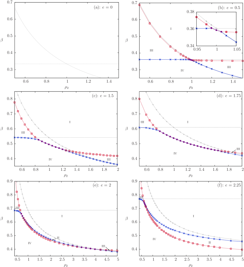
Figure 1: (Color online) The phase diagram in the ($\rho_{2}$, $\beta$)-plane for the model in (9) at 6 increasing values of the electric charge $e$ when $\rho_{1}=1$. Blue x markers ($\times$) connected with dashed lines are charged critical points, and red squares ($\square$) connected with dotted lines are the neutral critical points. When these critical points are merged, it is shown by filled squares ($\blacksquare$) in violet connected with solid lines. Moreover, with lines in silver color, we present critical points of one-component superconductors with $e$ as denoted in panel. The horizontal line is the critical line when $\rho=\rho_{1}=1$, and the plus markers ($+$) are the critical points when $\rho=\rho_{2}$. For these reference lines, the dashed and dotted line type correspond to charged and neutral critical points, as above. The inset in panel (b) is a magnification of the lines merger region. Phases are denoted by roman numbers. I. Ordered phase with spontaneously broken $U(1)\times U(1)$ symmetry, $m_{\textbf{A}}\neq 0,\Upsilon_{\mu,(1,-1)}\neq 0$. II. Spontaneously broken global $U(1)$ symmetry, with restored $U(1)$ gauge symmetry, $m_{\textbf{A}}=0,\Upsilon_{\mu,(1,-1)}\neq 0$. III. Spontaneously broken $U(1)$ gauge symmetry, with restored global $U(1)$ symmetry, $m_{\textbf{A}}\neq 0,\Upsilon_{\mu,(1,-1)}=0$. IV. Normal phase with fully restored $U(1)\times U(1)$ symmetry, $m_{\textbf{A}}=0,\Upsilon_{\mu,(1,-1)}=0$. The system size considered is $32^{3}$. Except for inset, error bars are smaller than marker size and thus omitted from diagram.

IV.1 Topological excitations

Consider now the case when the neutral critical line is situated above the charged critical line, that is, when going from phase I ($U(1)\times U(1)$ broken symmetry) to phase III (broken $U(1)$ charged symmetry) across the neutral phase transition line in Fig. 1. This phase transition is driven either by proliferation of $(0,1)$ or $(1,0)$ vortices. The composite $(1,1)$ vortices do not couple to the neutral sector of Eq. (9) and can thus never be responsible for destroying the order in the neutral sector. The other composite topological excitation $(1,-1)$ is, by inspection of (9), seen to have neither energetic nor entropic advantage over individual vortices. Because the vortices $(1,0)$, $(0,1)$ cost the same amount of energy in the neutral sector, but the vortex with lowest stiffness $\rho_{j}$ costs less energy in the charged sector, the neutral critical line must be associated with proliferation of individual vortices of the component with the smallest value of the bare stiffness $\rho_{j}$, when going from phase I to phase III. This phase transition is, outside the region where there is a strong competition between different kinds of vortex excitations, found to be of second order in the 3Dxy universality class.prb05 When the individual vortices proliferate, the corresponding stiffness is renormalized to zero and the remaining condensate will be a charged condensate with order in the remaining component. Thus, the remaining condensate will, at a higher temperature, have a phase transition similar to that of a one-component superconductor,

$$F_{III\rightarrow IV}^{\textnormal{eff}}=\frac{\rho_{j}}{2}(\nabla\theta_{j}-e\textbf{A})^{2}+\frac{(\nabla\times\textbf{A})^{2}}{2},$$ (32)

where $j$ now is the index of the component with largest stiffness $\rho_{j}$.

This is verified in Fig. 1 by observing that the charged critical line between III and IV asymptotically approaches the one-component reference lines away from the region of competition between different kinds of topological excitations. This phase transition is second order of the inverted 3Dxy universality class.prb05

When there is a transition from phase I ($U(1)\times U(1)$ broken symmetry) to phase II (broken $U(1)$ neutral symmetry) in panel (e) and (f) of Fig. 1, the charged critical point is situated at a lower temperature than the neutral critical point. In this case the topological defects responsible for the phase transition are $(1,1)$ vortices, because the other possible vortices will destroy order in the neutral sector of Eq. (9), and thus are not proliferating at this transition line. As discussed in Sec. II.2, the $(1,1)$ vortices proliferating from an ordered background may be mapped onto a single component superconductor with effective stiffness (if to neglect their internal structure) $\rho^{\prime}=\rho_{1}+\rho_{2}$,

$$F_{I\rightarrow II}^{\textnormal{eff}}=\frac{\rho_{1}+\rho_{2}}{2}(\nabla\theta-e\textbf{A})^{2}+\frac{(\nabla\times\textbf{A})^{2}}{2}.$$ (33)

In Fig. 2 we show results when bare component stiffnesses $\rho_{j}$ are kept fixed, and electric charge $e$ is varied. In panel (a), we also present a one-component reference line corresponding to the phase transition of the superconductor in (33). Indeed, away from the splitting point, the transition from I to II approaches this reference line, and the actual second order phase transition is of the inverted 3Dxy universality class. Note that the mapping in (33) yields a one-component superconductor with stiffness $\rho_{1}+\rho_{2}$ that always is stiffer than the two reference lines in Fig. 1 (which are one-component superconductors with stiffness $\rho_{1}$ and $\rho_{2}$). Thus, the charged transition line between phase I and phase II is always lower than the reference lines in Fig. 1. Phase II in Fig. 1 and 2 is the metallic superfluid phase (i.e. exhibiting order only in the gauge invariant phase difference) discussed in Sec. II.2 and the effective free energy in the remaining superfluid condensate is given in Eq. (11). The cheapest topological defects that proliferate at higher temperatures and destroy the remaining composite order in this phase, are individual vortices. Hence, away from the region of competing topological defects (i.e. away from the splitting point), the transition line from phase II to phase IV should be similar to a one-component superfluid with effective stiffness $\rho^{\prime}=\rho_{1}\rho_{2}/(\rho_{1}+\rho_{2})$,

$$F_{II\rightarrow IV}^{\textnormal{eff}}=\frac{\rho_{1}\rho_{2}}{2(\rho_{1}+\rho_{2})}(\nabla\theta)^{2}.$$ (34)

Note that in both panels of Fig. 2, the neutral transition line between II and IV is found to be asymptotically independent of $e$, thus approaching a constant value asymptotically far away from the region of competition with different vortices, as Eq. (34) suggests. Moreover, Eq. (34) predicts the value $\beta=\beta_{c}(\rho_{1}+\rho_{2})/(\rho_{1}\rho_{2})$ of the actual line, which corresponds well with the results in the figure. Here, $\beta_{c}\approx 0.334$ is the critical point of the one component superfluid ($e=0$) when $\rho=1$.

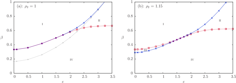
Figure 2: (Color online) The phase diagram in the ($\beta$, $e$)-plane for the two component 3D London model (9) with $\rho_{1}=1$ and for two different values of $\rho_{2}$. In the left diagram is $\rho_{2}=\rho_{1}=\rho=1$, whereas $\rho_{2}=1.15$ in the right diagram, i.e. there is a moderate disparity. Markers and line types are the same as in Fig. 1, i.e. blue x markers ($\times$) connected with dashed lines are charged critical points, red squares ($\square$) connected with dotted lines are neutral critical points, filled squares ($\blacksquare$) in violet connected with solid lines are merged transitions. The silvered plus markers ($+$) in the left diagram is a one-component reference line of a superconductor with bare stiffness $2\rho$ and charge $e$. Roman numbers denote the different phases as given in the caption of Fig. 1. Note that these diagrams are 2D cross sections of a 3D phase diagram in ($\beta$, $\rho_{2}$, $e$)-space perpendicular to the cross sections in Fig. 1. The lattice size is $32^{3}$. Errors are smaller than marker size and thus omitted from diagram.

Note that vortices on the form $(n_{1},n_{2})$ with $n_{j}\geq 1$, $n_{k\neq j}>1$ can, by inspection of (9), be shown to always be energetically unfavourable compared with other topological excitations in this model. Such higher order vortices are thus not relevant when $\rho_{d}=0$ and $e_{1}=e_{2}=e$.

IV.2 Gauge field fluctuation driven merger of the phase transitions in case of unequal bare stiffnesses

We next discuss the evolution of the phase diagrams in Fig. 1 and 2 when $e$ is varied. When charge increases, the energy of the composite $(1,1)$ vortices (which have no topological charge in the neutral sector), as well as the energy associated with charged currents of individual vortices decrease. This leads to a formation of a region in the phase diagram which is characterized by a merger of the two $U(1)$ transitions in the case of unequal bare stiffnesses of the two condensates. Thus, even in the case of unequal stiffnesses, when the coupling to a fluctuating noncompact gauge field is sufficiently strong, there appears a phase transition directly from the ordered phase with spontaneously broken $U(1)\times U(1)$ symmetry to the fully disordered normal phase. See also discussions of transition mergers caused by other kinds of couplings in Refs. kuklovAB, ; chernodub, ; eskil1, . Panel (b) of Fig. 2 clearly illustrates this behavior. In this panel, the value of bare stiffness disparity is fixed when $e$ increases. For low values of $e$ there are two phase transitions: At lower temperature individual vortices with lower stiffness proliferate while at higher temperature a proliferation of individual vortices of stiffer condensate takes place. However, when $e$ increases, the two lines approach each other and merge at $e\approx 1.3$.

The line merger is a consequence of the fact that at a substantially large electric charge, the bare energy of an individual vortex in a broken $U(1)\times U(1)$ phase is dominated by the neutral mode. Because a proliferation of less energetically expensive individual defects destroys the neutral mode, this eliminates the bare long-range logarithmic interaction between vortices in the stiffer condensate, leading to a dramatic decrease in their bare line tension and thus to their preemptive proliferation. On the other hand in a range of parameters a proliferation of composite $(1,1)$ vortices can trigger proliferation of individual vortices again leading to a “preemptive” restoration of the full $U(1)\times U(1)$ symmetry via a single phase transition. When electric charge is increased further, then eventually at a certain point in the interval $e\in(1.75...1.875)$ the $(1,1)$ vortices become much less energetically expensive than other excitations and can proliferate at low temperatures without triggering a proliferation of individual vortices. Then the metallic superfluid phase (II) emerges as discussed in Sec. II.2.

IV.3 Order of the phase transition associated with the merged lines

Let us now characterize the phase transition along the merged lines of Fig. 1 and 2. In Ref. kuklov, , using the ${\bf j}$-current model the transition line from $U(1)\times U(1)$ to fully symmetric state in the case of equal stiffnesses presented in panel (a) of Fig. 2, was found to be a first order transition. We obtain consistent results in our Villain-model based simulations.

Furthermore in Fig. 3, we report the simulation results associated with the merged line in a case when bare stiffnesses are not equal. We find a first order transition along the merged line in our case when there is a disparity of the bare phase stiffnesses. This shows that the first order phase transition in a $U(1)\times U(1)$ non-compact gauge theory is not related to the specific degeneracy of the model with equal stiffnesses $\rho_{1}=\rho_{2}$, but appears to be related to the case when there are several competing or composite topological defects.

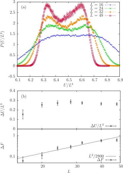
Figure 3: (Color online) (a): Histograms for the probability distribution of the internal energy per site $U/L^{3}$ at $\beta\approx 0.487$ when parameters are $\rho_{1}=1$, $\rho_{2}=1.05$ and $e=1.5$. This is the merged transition point found in Fig. 1 at ($\rho_{2}$, $\beta$) = (1.05, 0.487) in panel (c). A double-peak structure develops when $L$ increases. (b): Upper panel shows that the finite size scaling of the latent heat per site $\Delta U/L^{3}$ approaches a finite value when $L$ increases. This is the distance between the peaks in (a). The lower panel shows the finite size scaling of the difference in the free energy, $\Delta F=(1/\beta)\ln(P_{\textnormal{max}}/P_{\textnormal{min}})$ taken between the double peak value $P_{\textnormal{max}}$ and the value of the minimum in between $P_{\textnormal{min}}$ of the histograms in (a). For a first order phase transition, $\Delta F\sim L^{d-1}$.Lee_90_91 Ferrenberg-Swendsen reweighting was used to obtain histograms with similar height peaks.Ferrenberg_88

V Monte Carlo simulation, general model with both gauge field and dissipationless drag interactions

Next, we present results from Monte Carlo simulations when both drag and gauge field mediated interactions are included.

V.1 Competing gauge field and drag interactions in the case $\rho_{1}=\rho_{2}=1$

In Figure 4, we present results for the case when the bare component stiffnesses are equal $\rho_{1}=\rho_{2}=\rho=1$, and the gauge field couplings are equal, $e_{1}=e_{2}=e$. We vary the inverse temperature $\beta$ and the bare drag coefficient $\rho_{d}$ and map out the phase diagram in the $(\beta,\beta\rho_{d})$-plane for a number of different values of $e$. We consider positive $\rho_{d}$ only. In this specific case, the charged and neutral modes in (5) are written,

$$\begin{split}F=\frac{1}{2}\Bigg{[}&\frac{\rho-2\rho_{d}}{2}(\nabla\theta_{1}-\nabla\theta_{2})^{2}\\ &+\frac{\rho}{2}(\nabla\theta_{1}+\nabla\theta_{2}-2e{\bf A})^{2}+(\nabla\times{\bf A})^{2}\Bigg{]}.\end{split}$$ (35)

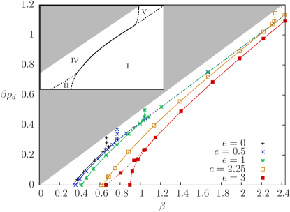
Figure 4: (Color online) Phase diagram in the ($\beta$, $\beta\rho_{d}$) plane with competing gauge field and drag interactions. Results are given for five different values of the charge $e_{1}=e_{2}=e$. The bare component stiffnesses are equal, $\rho_{1}=\rho_{2}=1$, and the system size considered is $32^{3}$. The gray-shaded area is the prohibited region by the stability condition, Eq. (8). Line type corresponds to character of phase transition as in Fig. 1, that is, charged lines are dashed, neutral lines are dotted and merged transition lines are solid. Except for this, lines are guide to the eye, only. The inset in the figure shows the schematic structure of the phases in the diagram for all cases with $e>0$. Roman numbers denote phases. Phases I, II and IV are the same as given in the caption of Fig. 1, whereas V is, similar to phase III in Fig. 1, a phase with spontaneously broken $U(1)$ gauge symmetry, and restored global $U(1)$ symmetry, $m_{\textbf{A}}\neq 0,\Upsilon_{\mu,(1,-1)}=0$. However, in V the broken $U(1)$ gauge symmetry is associated with composite phase sum, whereas in phase III of Fig. 1, it is associated with the phase of the single ordered component. For the given ranges of the phase diagram, II is only found for $e=2.25$ and $e=3$ and V is not found for $e=3$. When $e=0$, all phase transitions are neutral and phase II and V are associated with broken global $U(1)$ symmetry in the phase difference and phase sum, respectively.eskil1 The results for $e=0$ are here simulated with a fluctuating gauge field, and coincide (as they should) with the equal stiffnesses results in Ref. eskil1, with no fluctuating gauge field.

Here, we have the interesting situation where drag- and gauge field mediated intercomponent long-range vortex interactions are found to be of opposite signs, see Eq. (18). Thus, the drag coupling $\rho_{d}\neq 0$, when significantly strong, favors formation of the $(1,-1)$ composite vortices (via a mechanism similar to that in Ref. eskil1, ). On the other hand, the gauge field coupling favors the formation of $(1,1)$ bound states of individual vortices when $e_{1}$ and $e_{2}$ are of the same sign. This competition is studied in Fig. 4. Its most striking consequence is that it leads to the existence of four phases: At strong drag there is a superconducting phase where a neutral mode is destroyed by the proliferated $(1,-1)$ vortices (Phase V). At strong electric charge there is a superfluid phase with proliferated $(1,1)$ vortices (Phase II).

We next consider these phases more closely. The results in Fig. 4 show that the phase V appears when $(1,-1)$ vortices proliferate and thus there is no longer a broken symmetry in the neutral sector of Eq. (35). Note that when we are well above the region of competing topological defects in Fig. 4, then, by neglecting the internal vortex structure, we may approximate the $(1,-1)$ vortices to map onto vortices in a one component superfluid with stiffness $\rho^{\prime}=2(\rho-2\rho_{d})$,

$$F_{I\rightarrow V}^{\textnormal{eff}}=(\rho-2\rho_{d})(\nabla\theta)^{2}.$$ (36)

This effective limiting model is $e$-independent. Indeed this physics manifests itself in the fact that in Fig. 4, the actual transition is seen to approach asymptotically the reference line $\beta\rho_{d}=(\beta-\beta_{c}/2)/2$.

In Sec. IV, the superconducting phase III, which similarly to phase V exhibits charged order and neutral disorder, was created from the fully ordered phase by proliferation of individual vortices when we increased disparity in the bare stiffness of the two components. Here, phase V is created by proliferation of composite vortices, and the coupling constant responsible for creating the phase is $\rho_{d}$. Consequently, the remaining order is now in the gauge invariant phase difference of the charged mode, given by second and third terms in (35). On the other hand, phase III exhibits order in the gauge invariant phase difference of the component with largest bare stiffness. Note also that in the $U(1)\times U(1)$ (Phase I) state with equal stiffnesses the $(1,0)$, $(0,1)$ vortices carry half of the magnetic flux quanta.prl02 It can be seen from (35) that in the phase V $(1,0)$, $(0,1)$ vortices become equivalent and no longer have logarithmic divergence of internal energy per unit length due to absence of a neutral mode. I.e. they become similar to Abrikosov vortices, but carry only a half quantum of magnetic flux. This phenomenon is related to the fractionalization of superfluid velocity quantum in the metallic superfluid state.nphys From (35) it also follows that the individual vortices behave as vortices in a one component superconductor with effective stiffness $\rho^{\prime}=\rho/2$ and double effective charge $e^{\prime}=2e$,

$$F_{V\rightarrow IV}^{\textnormal{eff}}=\frac{\rho}{4}(\nabla\theta-2e\textbf{A})^{2}+\frac{(\nabla\times\textbf{A})^{2}}{2}.$$ (37)

In Fig. 4, the transition from the phase V to the normal phase IV is indeed found to tend asymptotically to a phase transition one would predict from the model (37). For this model, the transition line is found to be vertical, in accordance with the drag independent stiffness in (37). Note that when $e$ increases, the critical temperature of the vortex loop proliferation is decreased and the vertical line moves to the right in Fig. 4.

Next, the phase II may be investigated in a similar way as the phase V above. Phase II appears when $(1,1)$ vortices proliferate. As discussed in section IV, the remaining order is in the neutral sector of (5) and the transition to the normal state is governed by proliferation of individual vortices that asymptotically behave as a one-component superfluid with effective stiffness $\rho^{\prime}=(\rho-2\rho_{d})/2$,

$$F_{II\rightarrow IV}^{\textnormal{eff}}=\frac{\rho-2\rho_{d}}{4}(\nabla\theta)^{2}.$$ (38)

The critical phase transition of this condensate will follow the line $\beta\rho_{d}=(\beta-2\beta_{c})/2$. Indeed, this is the case for $e=3$ in Fig. 4 away from the region with competing topological defects.

Similarly to Sec. IV we find evidence of a first order transition when lines are merged and $e>0$, as seen in Fig. 5. When only drag or gauge field is included in a two-component system, first-order transitions may emerge.eskil1 ; kuklov ; steinar Our results show that the first-order character of this phase-transition line persists also in the case where both of the interactions are present and competing.

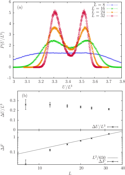
Figure 5: (Color online) (a): Histograms for the probability distribution of the internal energy per site $U/L^{3}$ at the critical point when parameters are $\rho_{1}=\rho_{2}=\rho=1$, $e_{1}=e_{2}=e=1$ and $\rho_{d}=0.4$. This is a merged transition point at ($\beta$, $\beta\rho_{d}$) = (0.948, 0.379) along the critical line for $e=1$ in Fig. 4. A pronounced double-peak structure is found to develop when $L$ increases. (b): Upper panel shows the finite size scaling of the latent heat per site $\Delta U/L^{3}$. This is the distance between the peaks in (a). The lower panel shows the finite size scaling of the difference in the free energy, $\Delta F=(1/\beta)\ln(P_{\textnormal{max}}/P_{\textnormal{min}})$ taken between the double peak value $P_{\textnormal{max}}$ and the value of the minimum in between $P_{\textnormal{min}}$ of the histograms in (a). For a first order phase transition, $\Delta F\sim L^{d-1}$.Lee_90_91 Ferrenberg-Swendsen reweighting was used to obtain histograms with peaks of similar height.Ferrenberg_88

V.2 The regime where gauge field and drag interactions both favor formation of similar paired phase

In Fig. 6 we present the phase diagram in the case when $\rho_{1}=\rho_{2}=\rho=1$ and $e_{1}=-e_{2}=e=1$. The separation in neutral and charged modes is now,

$$\begin{split}F=\frac{1}{2}\Bigg{[}&\frac{\rho-2\rho_{d}}{2}(\nabla\theta_{1}-\nabla\theta_{2}-2e{\bf A})^{2}+(\nabla\times{\bf A})^{2}\\ &+\frac{\rho}{2}(\nabla\theta_{1}+\nabla\theta_{2})^{2}\Bigg{]}.\end{split}$$ (39)

The motivation for investigating this particular case is found in the off-diagonal elements of the matrix in Eq. (18) where the interactions originating with the gauge field will act in unison with the bare drag interactions upon switching the sign of the electric charge in one of the components (in contrast to the situation considered in the previous section). Indeed such a regime should lead to the growth of the paired (MSF) phase in the phase diagram.

Consider the simulation results shown in Fig. 6. For comparison, we include the results when there is no gauge field coupling, $e_{1}=e_{2}=0$, and when gauge field coupling competes with the drag interaction, $e_{1}=e_{2}=1$. First notice that the paired phase which appears when charges are opposite, is the metallic superfluid phase (VI) which now is associated with spontaneously broken global $U(1)$ symmetry in the phase sum (and not the phase difference as in Fig. 1, 2 and 4). Positive drag will favor $(1,-1)$ vortices as before. However, because of the change of sign of one of the charges, the $(1,-1)$ vortices are now associated with the charged sector of Eq. (39). The $(1,1)$ vortices are associated with the neutral mode, and thus the neutral critical point is determined by the onset of the associated helicity modulus $\Upsilon_{\mu,(1,1)}$. The gauge field renders the $(1,-1)$ vortices the topological objects with lowest excitation energy. When they proliferate the superconducting sector is destroyed. Asymptotically, the associated phase-transition line is therefore expected to follow the behavior of a one-component superconductor with $\rho^{\prime}=2(\rho-2\rho_{d})$ and effective charge $e$,

$$F_{I\rightarrow VI}^{\textnormal{eff}}=(\rho-2\rho_{d})(\nabla\theta-e\textbf{A})^{2}+\frac{(\nabla\times\textbf{A})^{2}}{2}.$$ (40)

The remaining condensate will have superfluidity destroyed via proliferation of individual vortices which asymptotically can be mapped onto a one-component superfluid with stiffness $\rho^{\prime}=\rho/2$,

$$F_{VI\rightarrow IV}^{\textnormal{eff}}=\frac{\rho}{4}(\nabla\theta)^{2}.$$ (41)

his is the exact same behavior as expected when $e=0$, which is also confirmed by simulations in Fig. 6. Note that there is neither $\rho_{d}$ nor $e$ dependence of this line.

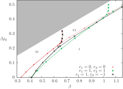
Figure 6: Phase diagram in the ($\beta$, $\beta\rho_{d}$) plane of the general model when $\rho_{1}=\rho_{2}=1$ for the case of different charges $e_{1}=-e_{2}=1$. These are the black x markers ($\times$) and the line type denotes charged, neutral and merged critical lines by dashed, dotted and solid lines as in Fig. 1, 2 and 4. Roman numbers denote the phases of this particular case, $e_{1}=-e_{2}=1$. I. Ordered phase with spontaneously broken $U(1)\times U(1)$ symmetry, $m_{\textbf{A}}\neq 0,\Upsilon_{\mu,(1,1)}\neq 0$. IV. Normal phase with fully restored $U(1)\times U(1)$ symmetry, $m_{\textbf{A}}=0,\Upsilon_{\mu,(1,1)}=0$. VI. Spontaneously broken global $U(1)$ symmetry, with restored $U(1)$ gauge symmetry, $m_{\textbf{A}}=0,\Upsilon_{\mu,(1,1)}\neq 0$. For comparison, the results of the two cases $e_{1}=e_{2}=0$, $1$, from Fig. 4, are presented. The phases for these two cases follow from the inset and caption of Fig. 4. The lines are guide to the eye. The system size considered is $32^{3}$. The uncertainties in the position of the phase-transition lines are smaller than the marker size, and are omitted from the diagram.

Fig. 6 also shows that when gauge field and drag act in unison it amounts to a small increase of the region of paired phase compared to the case when there is only drag interaction. However when interactions compete there is a stronger effect of the suppression of the corresponding paired phase. Also note that the cases $e_{1}=-e_{2}=1$ and $e_{1}=e_{2}=1$ coincide when $\rho_{d}=0$. This is readily inferred from Eq. 1, since when $\rho_{d}=0$, one model can be mapped onto another by change in sign of charges $e_{j}$ accompanied by a sign-change of one of the phases $\nabla\theta_{j}$.

VI Conclusion

We have considered a three-dimensional lattice superconductor model in the London limit, with two individually conserved condensates. These condensates interact with each other by two mechanisms. The first is a dissipationless Andreev-Bashkin drag term representing a current-current interaction. The second is a fluctuating gauge field. Intercomponent Josephson coupling is absent on symmetry grounds. Such models are relevant in a number of physical circumstances ranging from the theories of the quantum ordered states of metallic hydrogen, models of neutron stars, and were earlier suggested as effective models describing valence bond solid to Neel quantum phase transition in the proposed theories of deconfined quantum criticality.

In the case when there is no intercomponent drag, $\rho_{d}=0$, and component charges are equal, $e_{1}=e_{2}=e$ and there is a disparity of the bare component stiffnesses, we find that a sufficiently strong coupling to a non-compact gauge field causes a merger of phase-transition lines. This yields a direct transition from broken $U(1)\times U(1)$ to normal state even when the bare component stiffnesses are unequal. When the charge $e$ is increased, the merger occurs for a higher disparity of stiffnesses. However, a further increase of the coupling beyond a certain critical strength results in a new splitting of the transition line. This yields a metallic superfluid phase. The merger of the $U(1)$ transition lines is associated with a competition between different kinds of topological defects where proliferation of one type of vortices triggers a “preemptive” proliferation of another. The result is a much more complex picture of the behavior of topological defects in the phase transition than in singel-component $U(1)$ models. The second splitting is due to the fact that increased coupling to the non-compact gauge field decreases the free energy per unit length of a bound state of topological defects. The bound state in question (a composite vortex) has a topological charge only in the charged sector of the model. This in turn results in increased suppression of the critical stiffness associated with the charged sector of the theory, which eventually undergoes a symmetry-restoring phase transition before the neutral sector.

We find that also when the bare stiffnesses are unequal, the merged phase transition is first-order in character. Note that previously first order transitions were reported in the $U(1)\times U(1)$ gauge theory with degenerate stiffnesses,kuklov ; steinar $U(1)\times U(1)$ models with a compact gauge-field, as well as to phase transitions in the $SU(2)$ model with noncompact Abelian gauge field. chernodub

At stronger coupling, far away from the region of merged lines phase diagram exhibits 3Dxy (neutral) or inverted 3Dxy (charged) critical points.

In the main part of the paper, we have performed a study of the phase diagram of the generic $U(1)\times U(1)$ lattice London gauge model featuring both gauge field and direct non-dissipative drag interactions. We have obtained, through large-scale Monte Carlo simulations, its phase diagram as a function of these two generic coupling constants.

For the case where the bare component stiffnesses and charges are equal, $\rho_{1}=\rho_{2}=1$ and $e_{1}=e_{2}=e$, we find the formation of two different paired phases as a result of a competition between gauge-field and intercomponent drag couplings. High values of drag produce a composite superconducting phase associated with a broken local $U(1)$ gauge symmetry in the phase sum. There, the theory effectively features a doubled electric charge compared with $U(1)\times U(1)$ phase, cf. Eq. (37). At high values of $e$, the gauge field coupling wins over the drag coupling, yielding a paired superfluid phase (the metallic superfluid) associated with the order in the gauge invariant phase difference. In between these two different phases, there is a region with a direct transition from broken $U(1)\times U(1)$ to normal state which exhibits clear-cut signatures of a first-order transition, cf. the transition line connecting regions II and V in Fig. 4.

For comparison, we also reported a quantitative study of the situation where gauge-field mediated intercomponent interactions and intercomponent drag both favor metallic superfluid phase.

Appendix A The $N$-component model

We may easily generalize to the case of arbitrary number of components $N$. Again, the action will be given on the form

$$Z=\int\mathcal{D}\theta_{1}...\int\mathcal{D}\theta_{N}\int\mathcal{D}\textbf{A}\quad\mathrm{e}^{-S},$$

$$\begin{split}S&=\frac{\beta}{2}\int d^{3}r\Big{\{}[\nabla\times\textbf{A}(\textbf{r})]^{2}\\ &\quad+[\nabla\theta_{j}(\textbf{r})-e_{j}\textbf{A}(\textbf{r})]R_{jk}[\nabla\theta_{k}(\textbf{r})-e_{k}\textbf{A}(\textbf{r})]\Big{\}}.\end{split}$$ (42)

The matrix $R_{jk}$ is in general given by

$$R_{jk}=\left(\rho_{j}-\sum_{l}\rho_{d,jl}\right)\delta_{jk}+\rho_{d,jk},$$ (43)

where $\rho_{d,jk}$ is the drag-coefficient between components $j$ and $k$, obviously, $\rho_{d,jk}=\rho_{d,kj}$ and $\rho_{d,jk}=0$ when $j=k$. Following exactly the same procedure as in the case $N=2$, we arrive at the $N$-component action

$$\begin{split}S=\frac{\beta}{2}\int d^{3}q&\Bigg{[}\textbf{U}_{j}(\textbf{q})\left(R_{jk}-\frac{e_{l}e_{m}R_{lj}R_{mk}}{q^{2}+m_{0}^{2}}\right)\textbf{U}_{k}(-\textbf{q})\\ &\quad+\tilde{\textbf{A}}(\textbf{q})(q^{2}+m_{0}^{2})\tilde{\textbf{A}}(-\textbf{q})\Bigg{]},\end{split}$$ (44)

where the Fourier transform of $\nabla\theta_{j}(\textbf{r})$, is denoted by $\textbf{U}_{j}(\textbf{q})$, and

$$m_{0}^{2}=e_{j}R_{jk}e_{k}.$$ (45)

This expression is seen to reproduce the case $N=2$ given in Eq. (7). The gauge field is integrated out and the dualization now follows the same path as previously, yielding

$$Z=\sum_{\textbf{m}_{1}}...\sum_{\textbf{m}_{N}}\quad\mathrm{e}^{-S},$$

$$S=2\beta\pi^{2}\int d^{3}q\;\textbf{m}_{j}(\textbf{q})V_{jk}(q^{2})\textbf{m}_{k}(-\textbf{q}),$$ (46)

where the vortex interactions are given by

$$V_{jk}(q^{2}) =\frac{1}{q^{2}}\left(R_{jk}-\frac{e_{l}e_{m}R_{lj}R_{mk}}{q^{2}+m_{0}^{2}}\right)$$

$$=\frac{R_{jk}-\frac{e_{l}e_{m}R_{lj}R_{mk}}{m_{0}^{2}}}{q^{2}}+\frac{\frac{e_{l}e_{m}R_{lj}R_{mk}}{m_{0}^{2}}}{q^{2}+m_{0}^{2}}.$$ (47)

This is seen to be on precisely the same form as Eq. (18) for the case $N=2$. Following Appendix B in Ref. prb05, , a dualization of the corresponding two-component lattice model in Eq. (21) may be performed to yield the exact same result as in (46) and (47) where the vortex fields now are defined on the vertices of the Fourier space dual lattice and $q^{2}\rightarrow|\textbf{Q}_{\textbf{q}}|^{2}$.

Appendix B Gauge field correlator

By adding source term and Fourier transformation of the model in Eq. (42), the generating functional for deriving the gauge field correlator reads

$$Z_{J}=\int\mathcal{D}\theta_{1}...\int\mathcal{D}\theta_{N}\int\mathcal{D}\textbf{A}\quad\mathrm{e}^{-S},$$

$$\begin{split}S_{J}=&\frac{\beta}{2}\int d^{3}q\Big{\{}\frac{1}{\beta}\left[\textbf{J}(\textbf{q})\textbf{A}(-\textbf{q})+\textbf{A}(\textbf{q})\textbf{J}(-\textbf{q})\right]\\ &+[\textbf{U}_{j}(\textbf{q})-e_{j}\textbf{A}(\textbf{q})]R_{jk}[\textbf{U}_{k}(-\textbf{q})-e_{k}\textbf{A}(-\textbf{q})]\\ &+q^{2}\textbf{A}(\textbf{q})\textbf{A}(-\textbf{q})\Big{\}},\end{split}$$ (48)

where $\textbf{J}(\textbf{q})$ are the electric currents that couples linearly to the gauge field in the source terms. Sum over repeated indices is assumed. We now proceed similar to Sec. II.3 by completing the squares of the gauge field and integrate out the shifted gauge field $\tilde{\textbf{A}}(\textbf{q})=\textbf{A}(\textbf{q})+(\textbf{J}(\textbf{q})/\beta-e_{j}R_{jk}\textbf{U}_{k}(\textbf{q}))/(q^{2}+m_{0}^{2})$ which yields

$$Z_{J}=\int\mathcal{D}\theta_{1}...\int\mathcal{D}\theta_{N}\quad\mathrm{e}^{-S},$$

$$\begin{split}S_{J}=&\frac{\beta}{2}\int d^{3}q\Bigg{\{}-\frac{\textbf{J}(\textbf{q})\textbf{J}(-\textbf{q})}{\beta^{2}(q^{2}+m_{0}^{2})}\\ &+\frac{\textbf{J}(\textbf{q})e_{j}R_{jk}\textbf{U}_{k}(-\textbf{q})+e_{j}R_{jk}\textbf{U}_{k}(\textbf{q})\textbf{J}(-\textbf{q})}{\beta(q^{2}+m_{0}^{2})}\\ &+\textbf{U}_{j}(\textbf{q})\left(R_{jk}-\frac{e_{l}e_{m}R_{lj}R_{mk}}{q^{2}+m_{0}^{2}}\right)\textbf{U}_{k}(-\textbf{q})\Bigg{\}}.\end{split}$$ (49)

We now employ the constraint $\nabla\cdot\textbf{J}(\textbf{r})=0$, i.e. the electrical currents are divergence-free, such that components parallel to q are unphysical. Thus, the physical components of $\textbf{J}(\textbf{q})$ in the first term of (49) are projected out with the transverse projection operator

$$P_{T,\mu\nu}=\delta_{\mu\nu}-\frac{q_{\mu}q_{\nu}}{q^{2}}.$$ (50)

As discussed in Sec. II.3, we disregard the longitudinal part of $\textbf{U}_{j}(\textbf{q})$ and introduce the Fourier transformed vortex fields by (16). Thus, the generating functional is written

$$Z_{J}=\sum_{\textbf{m}_{1}}...\sum_{\textbf{m}_{N}}\quad\mathrm{e}^{-S_{0}-S_{1}},$$

$$S_{0}=2\beta\pi^{2}\int d^{3}q\;\textbf{m}_{j}(\textbf{q})V_{jk}(q^{2})\textbf{m}_{k}(-\textbf{q}),$$

$$\begin{split}S_{1}=\int d^{3}q&\Bigg{\{}\frac{i\pi e_{j}R_{jk}\varepsilon_{\mu\nu\eta}q_{\nu}}{q^{2}(q^{2}+m_{0}^{2})}\\ &\;\times\left[m_{\eta,j}(\textbf{q})J_{\mu}(-\textbf{q})-J_{\mu}(\textbf{q})m_{\eta,j}(-\textbf{q})\right]\\ &-\frac{J_{\mu}(\textbf{q})P_{T,\mu\nu}J_{\nu}(-\textbf{q})}{2\beta(q^{2}+m_{0}^{2})}\Bigg{\}},\end{split}$$ (51)

where $V_{jk}(q^{2})$ is given by (47) and $\varepsilon_{\mu\nu\eta}$ is the Levi-Civita symbol.

The gauge field correlators are derived the standard way by functional derivation of the currents

$$\langle A_{\mu}(\textbf{q})A_{\nu}(-\textbf{q})\rangle =\frac{1}{Z_{0}}\frac{\delta^{2}Z_{J}}{\delta J_{\mu}(-\textbf{q})\delta J_{\nu}(\textbf{q})}\Bigg{|}_{\textbf{J}=\textbf{0}}$$

$$=\left\langle\frac{\delta^{2}\mathrm{e}^{-S_{1}}}{\delta J_{\mu}(-\textbf{q})\delta J_{\nu}(\textbf{q})}\Bigg{|}_{\textbf{J}=\textbf{0}}\right\rangle,$$ (52)

where $Z_{0}=Z_{J}|_{\textbf{J}=\textbf{0}}=\sum_{\textbf{m}_{1}}...\sum_{\textbf{m}_{N}}\mathrm{e}^{-S_{0}}$ and the brackets denote thermal average with respect to $Z_{0}$. The functional derivation is easily performed by expanding the exponential in series and keep terms of $\mathcal{O}(J^{2})$, the only terms that survives both derivation and $\textbf{J}=\textbf{0}$, to yield

$$\begin{split}\frac{\delta^{2}\mathrm{e}^{-S_{1}}}{\delta J_{\mu}(-\textbf{q})\delta J_{\nu}(\textbf{q})}\Bigg{|}_{\textbf{J}=\textbf{0}}&=\frac{4\pi^{2}e_{j}e_{l}R_{jk}R_{lm}\varepsilon_{\mu\alpha\beta}\varepsilon_{\nu\gamma\kappa}}{q^{4}(q^{2}+m_{0}^{2})^{2}}\\ &\;\quad\times q_{\alpha}q_{\gamma}m_{\beta,k}(\textbf{q})m_{\kappa,m}(-\textbf{q})\\ &\quad+\frac{P_{T,\mu\nu}}{\beta(q^{2}+m_{0}^{2})}.\end{split}$$ (53)

The product $\varepsilon_{\mu\alpha\beta}\varepsilon_{\nu\gamma\kappa}$ is evaluated by the determinant

$$\varepsilon_{\mu\alpha\beta}\varepsilon_{\nu\gamma\kappa}=\begin{vmatrix}\delta_{\mu\nu}&\delta_{\mu\gamma}&\delta_{\mu\kappa}\\ \delta_{\alpha\nu}&\delta_{\alpha\gamma}&\delta_{\alpha\kappa}\\ \delta_{\beta\nu}&\delta_{\beta\gamma}&\delta_{\beta\kappa}\end{vmatrix},$$ (54)

to yield

$$\begin{split}\langle A_{\mu}(\textbf{q})A_{\nu}(-\textbf{q})\rangle&=\frac{P_{T,\mu\nu}}{\beta(q^{2}+m_{0}^{2})}+\frac{4\pi^{2}e_{j}e_{l}R_{jk}R_{lm}}{q^{2}(q^{2}+m_{0}^{2})^{2}}\\ &\quad\times\langle P_{T,\mu\nu}\textbf{m}_{k}(\textbf{q})\textbf{m}_{m}(-\textbf{q})\\ &\quad\qquad-m_{\nu,k}(\textbf{q})m_{\mu,m}(-\textbf{q})\rangle,\end{split}$$ (55)

when (53) is inserted in (52). We now find the gauge field propagator by letting $\nu\rightarrow\mu$ in (55) and summing over repeated indices, thus

$$\begin{split}\langle\textbf{A}(\textbf{q})\textbf{A}(-\textbf{q})\rangle=&\frac{4\pi^{2}e_{j}e_{l}R_{jk}R_{lm}\langle\textbf{m}_{k}(\textbf{q})\textbf{m}_{m}(-\textbf{q})\rangle}{q^{2}(q^{2}+m_{0}^{2})^{2}}\\ &+\frac{2}{\beta(q^{2}+m_{0}^{2})}.\end{split}$$ (56)

The gauge field correlator of the two-component discrete model in Eq. (21) is found similarly to Appendix C in Ref. prb05, and the result is as given in (56) with $q^{2}\rightarrow|\textbf{Q}_{\textbf{q}}|^{2}$ and vortex fields defined on the vertices of the Fourier space dual lattice.

References

- (1) J. M. Kosterlitz and D. J. Thouless, J. Phys. C 6, 1181 (1973); J. M. Kosterlitz, ibid. 7, 1046 (1974).
- (2) C. Dasgupta and B. I. Halperin, Phys. Rev. Lett. 47, 1556 (1981).
- (3) K. Fossheim and A. Sudbø, Superconductivity: Physics And Applications (John Wiley & Sons, London, 2004).
- (4) M. E. Peskin, Ann. Phys. (N.Y.) 113, 122 (1978); P. R. Thomas and M. Stone, Nucl. Phys. B 144, 513 (1978).
- (5) E. Babaev, arxiv: cond-mat/0201547.
- (6) A. B. Kuklov and B. V. Svistunov, Phys. Rev. Lett. 90, 100401 (2003); A. Kuklov, N. Prokof’ev, and B. Svistunov, ibid. 92, 030403 (2004).
- (7) E. Babaev, A. Sudbø, and N. W. Ashcroft, Nature 431, 666 (2004).
- (8) E. Smørgrav, E. Babaev, J. Smiseth, and A. Sudbø, Phys. Rev. Lett. 95, 135301 (2005).
- (9) J. Smiseth, E. Smørgrav, E. Babaev, and A. Sudbø, Phys. Rev. B 71, 214509 (2005).
- (10) A. Kuklov, N. Prokof’ev, B. Svistunov, arXiv:cond-mat/0501052; A. B. Kuklov, N. V. Prokof’ev, B. V. Svistunov, and M. Troyer, Ann. Phys. (N.Y.) 321, 1602 (2006).
- (11) S. Kragset, E. Smørgrav, J. Hove, F. S. Nogueira, and A. Sudbø, Phys. Rev. Lett. 97, 247201 (2006).
- (12) O. I. Motrunich and A. Vishwanath, Phys. Rev. B 70, 075104 (2004).
- (13) E. K. Dahl, E. Babaev, S. Kragset, and A. Sudbø, Phys. Rev. B 77, 144519 (2008).
- (14) M. N. Chernodub, E.-M. Ilgenfritz, and A. Schiller, Phys. Rev. B 73, 100506(R) (2006); M. Bock, M. N. Chernodub, E.-M. Ilgenfritz, and A. Schiller, ibid. 76, 184502 (2007); A. B. Kuklov, M. Matsumoto, N. V. Prokof’ev, B. V. Svistunov, and M. Troyer, Phys. Rev. Lett. 101, 050405 (2008); F.-J. Jiang, M. Nyfeler, S. Chandrasekharan, U.-J. Wiese, Journ. of Stat. Mech. 02, 02009 (2008).
- (15) E. Smørgrav, J. Smiseth, E. Babaev, and A. Sudbø, Phys. Rev. Lett. 94, 096401 (2005).
- (16) J. Smiseth, E. Smørgrav, and A. Sudbø, Phys. Rev. Lett. 95, 135301 (2005).
- (17) E. K. Dahl, E. Babaev, and A. Sudbø, Phys. Rev. B 78, 144510 (2008); Phys. Rev. Lett. 101, 255301 (2008).
- (18) A. F. Andreev and E. P. Bashkin, Sov. Phys. JETP 42, 164 (1975).
- (19) E. Babaev and N. W. Ashcroft, Nature Phys. 3, 530 (2007).
- (20) E. Babaev, Phys. Rev. Lett. 89, 067001 (2002).
- (21) P. B. Jones, Mon. Not. Royal Astr. Soc. 371, 1327 (2006); E. Babaev, Phys. Rev. Lett. 103, 231101 (2009).
- (22) T. Senthil, A. Vishwanath, L. Balents, S. Sachdev, and M. P. A. Fisher, Science 303, 1490 (2004).
- (23) For a review, see S. Sachdev, Nature Phys. 4, 173 (2008).
- (24) D. F. Agterberg and H. Tsunetsugu, Nature Phys. 4, 639 (2008); D. Podolsky, S. Chandrasekharan, and A. Vishwanath, Phys. Rev. B 80, 214513 (2009); A. Hu, L. Mathey, I. Danshita, E. Tiesinga, C. J. Williams, and C. W. Clark, Phys. Rev. A 80, 023619 (2009); E. Berg, E. Fradkin, and S. A. Kivelson, Nature Phys. 5, 830 (2009).
- (25) V. M. Kaurov, A. B. Kuklov, and A. E. Meyerovich, Phys. Rev. Lett. 95, 090403 (2005).
- (26) E. Babaev, L. D. Faddeev, and A. J. Niemi, Phys. Rev. B 65, 100512(R) (2002).
- (27) Note that in the solutions for fractional flux vortices in the Ginzburg-Landau model, the magnetic field is not exponentially localized. This affects intervortex interactions, see E. Babaev, J. Jaykka, and M. Speight, Phys. Rev. Lett. 103, 237002 (2009). However, the field delocalization effect vanishes in the short-coherence length limit, considered in the present paper. Hence, in our case the London limit yields a good approximation to intervortex interaction potentials.
- (28) J. Villain, J. Phys. (Paris) 36, 581 (1975).
- (29) N. Metropolis, A. W. Rosenbluth, M. N. Rosenbluth, A. H. Teller, and E. Teller, J. Chem. Phys. 21, 1087 (1953); W. K. Hastings, Biometrika 57, 97 (1970).
- (30) K. Hukushima and K. Nemoto, J. Phys. Soc. Jpn. 65, 1604 (1996); D. J. Earl and M. W. Deem, Phys. Chem. Chem. Phys. 7, 3910 (2005).
- (31) W. Janke and K. Nather, Phys. Rev. B 48, 7419 (1993); H. Kleinert, Gauge Fields in Condensed Matter (World Scientific, Singapore, 1989) Vol. 1.
- (32) K. Hukushima, Phys. Rev. E 60, 3606 (1999).
- (33) A. K. Nguyen and A. Sudbø, Phys. Rev. B 58, 2802 (1998).
- (34) A. K. Nguyen and A. Sudbø, Phys. Rev. B 57, 3123 (1998).
- (35) J. Hove and A. Sudbø, Phys. Rev. Lett. 84, 3426 (2000); K. Kajantie, M. Laine, T. Neuhaus, A. Rajantie, and K. Rummukainen, Nucl. Phys. B 699, 632 (2004).
- (36) A. Kuklov, N. Prokof’ev, and B. Svistunov, Phys. Rev. Lett. 92, 050402 (2004).
- (37) J. Lee and J. M. Kosterlitz, Phys. Rev. Lett. 65, 137 (1990); Phys. Rev. B 43, 3265 (1991).
- (38) A. M. Ferrenberg and R. H. Swendsen, Phys. Rev. Lett. 61, 2635 (1988); 63, 1195 (1989). The software used to perform the reweighting analysis did not take into account the explicit temperature dependence of the Villain model. However, the temperature interval for which the histogram statistics were obtained was narrow, and we thus expect the error to be negligible, as was checked by comparing reweighted histograms with raw data histograms.